Towards a new technique of incoherent scatter signal processing.

Abstract

This paper offers a new technique of incoherent scattering signal processing. The technique is based on the experimentally observed comb structure of the spectral power of separate realizations. The technique implies determining the positions and amplitudes of peaks in separate realizations, the formation - on their basis - of the spectral power of an individual realization not distorted by the smoothing function, and a subsequent summation of such spectra for the realizations. The technique has been tested using data from the Irkutsk incoherent scatter radar, both for the case of the incoherent scattering from thermal irregularities of plasma and for the case of the aspect scattering from instabilities elongated with the geomagnetic field.

Institute of Solar-Terrestrial Physics,

POBox 4026, Irkutsk, 664033, Russia

(berng@iszf.irk.ru)

1 Introduction.

The incoherent scatter (IS) method is one of a number of ionospheric remote sensing techniques. The method provides geophysical parameters of the ionosphere over a wide height range (from 100 to 1000 km), with spatial and temporal resolution determined by the form of the sounding pulse, and by the particular procedure of processing the received signal [Holt et al., 1992]. The accuracy of geophysical parameters determination in this case is usually governed by many parameters: ionospheric parameters, and parameters of the receiver (for instance, the background noise temperature), the method of the received signal processing, the type of sounding signal, the received signal averaging time, and by the spectral resolution of the method (or by the delay resolution in the case of a correlational processing of the signal). Furthermore, it is often necessary to improve the spectral resolution without impairing the spatial resolution. A conventional approach in handling this problem involves using special (‘composite’) signals, with a subsequent special-purpose processing of the received signal [Farley,1972; Sulzer, 1993; Lehtinen,1986]. However, situations can at times arise where it is not appropriate to use composite pulses (from energy considerations or auxillary conditions, for example), so that it is necessary to have a technique which would work well with traditional (’simple’) pulsed signals.

There are currently two main techniques for processing the received backscattered signal: the correlational technique, and the spectral technique [Evans, 1963]. Since the correlation function (obtained by applying the former type of processing) and the spectral power of the received signal (obtained by applying the latter type of processing) are related by the Wiener-Khintchin theorem, the two types of processing are equivalent in principle.

This paper is concerned with the method of improving the spectral resolution of the incoherent scatter method, based on the properties of the received signal according to the data from the Irkutsk incoherent scatter (IS) radar without using composite sounding signals.

2 The existing technique for processing the signal, and experimental data

Let us consider the radar equation relating the spectral power of the scattered signal to fluctuation parameters of dielectric permittivity. Within the approximation of the single scattering, in the far zone of the antenna, the mean spectral power of the received signal $<|u(\omega)|^{2}>$ is defined by a statistical radar equation [Berngardt and Potekhin, 2000] which - under the assumption of the spatial homogeneity of the spectral density of the irregularities and its weak dependence on the modulus of the wave vector $\Phi(\nu,\overrightarrow{r},-\overrightarrow{e_{r}}k)=\Phi(\nu,\overrightarrow{e_{r}}r_{0}-\overrightarrow{e_{r}}2k_{0})$ reduces to:

$$<|u(\omega)|^{2}>=\int S(\omega-\nu)<|u_{teor}(\nu)|^{2}>d\nu$$ (1)

$$<|u_{teor}(\nu)|^{2}>=V_{0}\int\Phi(\nu,\overrightarrow{e_{r}}r_{0},-\overrightarrow{e_{r}}2k_{0})|g(\overrightarrow{e_{r}})|^{2}d\overrightarrow{e_{r}}$$ (2)

here $\Phi(\nu,\overrightarrow{r},\overrightarrow{k})=\int<\epsilon(t,\overrightarrow{r})\epsilon^{*}(t+\Delta t,\overrightarrow{r}+\Delta\overrightarrow{r})>exp(-i\nu t+i\overrightarrow{k}\Delta\overrightarrow{r})\frac{d\nu d\overrightarrow{k}}{(2\pi)^{4}}$ - is the steady-state spectral density of permittivity irregularities; $g(\overrightarrow{e_{r}})$ is the beam factor determined by the product of the beams of the transmit and receive antennas; $\overrightarrow{e_{r}}=\overrightarrow{r}/r$ is a unit vector in a given direction; $V_{0}$ is the sounding volume; $r_{0}$ is the mean distance to it; $k_{0}$ is the wave number of the sounding wave; and $<|u_{teor}(\omega)|^{2}>$ is the theoretical spectrum of backscattering not distorted by the smearing function $S(\omega)$.

The problem of improving the spectral resolution in this case implies using the deconvolution operation with the kernel $S(\omega)\approx|\int a(\omega-\nu)o(\nu)d\nu|^{2}$ determined by the form of the sounding signal and the receiving window and usually having the property:

$$\frac{dS(\omega)}{d\omega}=0;\,when\,\omega=0;\,\frac{d^{2}S(\omega=0)}{d\omega^{2}}<0,$$

that is, having only one maximum at the zero frequency.

Thus, formally, we need to define the $DECONV$ - deconvolution operation:

$$<|u_{teor}(\nu)|^{2}>=<|u(\omega)|^{2}>\,DECONV\,S(\omega-\nu)$$ (3)

To carry out such an operation we make use of the linearity of the averaging operation:

$$<|u_{teor}(\nu)|^{2}>=<|u(\omega)|^{2}\,DECONV\,S(\omega-\nu)>.$$ (4)

Hence, to improve the spectral resolution, it is necessary to apply the deconvolution operation to each realization of spectral power and accumulate result spectrums over the realizations. Generally the problem (4) is not simpler compared with the initial one (3); however, in the case of its simplified solution, one may take advantage of the following experimental evidence of the structure of spectra of separate realizations.

Figure 1: Form of the spectral power of two successive realizations of the incoherently scattered signal (dotted line, and dashed line), mean spectral power (averaged over 1000 realizations, thick solid line), spectral density of the ’smearing’ function (dash-dotted line).

Figure 1 presents the structure of spectral power of two successive realizations of the scattered signal in sounding with the pulse of a duration of 750 ms and the length of the receiving window of 750 ms. For comparison, the figure also shows the form of the accumulated (averaged) spectral power, and the model form of the ’smearing’ function. Theoretically, the form of the smearing function depends on a large number of ionospheric parameters (on the electron density profile, on the experimental geometry with respect to the geomagnetic field), and can differ rather strongly from the model form [Shpynev, 2000]; however, the model form is applicable in the case of qualitative estimations.

It is apparent from the figure that the spectra of individual realizations differ rather strongly from one another, which suggests that the processes are occurring at a high rate when compared with the repetition frequency of sounding pulses, and is in agreement with existing data (the lifetime of thermal irregularities is on the order of 200 mks, which is significantly less than the interval between separate sounding runs - at the Irkutsk IS radar it is about 40 ms).

In spite of a relatively strong variability from realization to realization, the fine ’comb’ structure of the spectra is conserved. Consider the characteristics of such a comb structure. Figure 2 presents the frequency dependence of the amplitude of the peaks (solid line), the frequency dependence of the width of the peaks (line with circles), and a total number of peaks at a given frequency for the entire set of the realizations used in the analysis (line with triangles). It is evident from Figure 2 that the width of the peaks varies within 1-2 spectral widths of the sounding signal. The peaks are concentrated mainly in the band of the mean spectral power of the received signal, and the amplitude and occurrence frequency drop when the frequency of the peak is shifted with respect to the zero frequency.

3 Technique for solving the problem - deconvolution before an averaging.

The above characteristics of spectra of separate realizations of the received signal suggest that the initial (not convoluted with the smearing function) spectral power of the received signal has a comb structure with delta-shaped combs. Furthermore, the width of the peaks in the experimentally measured spectrum is determined solely by the properties of the smearing function. This permits us to relatively easily perform a deconvolution in (4). Indeed, within the framework of this assumption, a ’nonsmoothed’ spectral power of a separate realization has the form:

$$|u_{teor}(\omega)|^{2}=\begin{array}[]{c}N\\ \sum\\ i=1\end{array}A_{i}\delta(\omega-\omega_{i})$$ (5)

Then, within a constant factor, we have

$$|u(\omega_{j})|^{2}=\begin{array}[]{c}N\\ \sum\\ i=1\end{array}A_{i}S(\omega_{j}-\omega_{i})$$ (6)

We take into consideration that the function $S(\omega)$ is unknown but it is sufficiently narrowbanded when compared with a total spectral width $u(\omega)$, and the peaks in the spectral power of a separate realization are sufficiently isolated from each other, which permits us to neglect the influence of one peak on another. Then the amplitude of the observed peaks in $|u(\omega_{j})|^{2}$ will be proportional to the amplitude of the peaks in the ’nonsmeared’ spectrum $|u_{teor}(\omega)|^{2}$, and theirs location are the same:

$$|u(\omega_{j})|^{2}=S(0)A_{j}+o(\omega_{j})$$ (7)

where $o(\omega_{j})=\begin{array}[]{c}N\\ \sum\\ i=1\end{array}A_{i}S(\omega_{j}-\omega_{i})-S(0)A_{j}$ is a small addition which - in the case of a sufficient separation of the peaks (larger than the width of the smearing function $S(\omega)$)) becomes zero. In accordance with the expression (7), we determine the amplitudes $A_{i}$ and the frequencies $\omega_{i}$ from experimentally measured spectra $|u(\omega)|^{2}$, which corresponds to the solution of the system:

$$\left\{\begin{array}[]{c}\left.\frac{d}{d\omega}|u(\omega)|^{2}\right|_{\omega=\omega_{i}}=0\\ \left.\frac{d^{2}}{d\omega^{2}}|u(\omega)|^{2}\right|_{\omega=\omega_{i}}<0\\ A_{i}=|u(\omega_{i})|^{2}\end{array}\right.$$ (8)

Upon determining in this way the set of pairs of the parameters $A_{i}$ and $\omega_{i}$, it is also possible to obtain the ’nonsmeared’ spectrum of a single realization $|u_{teor}(\omega)|^{2}$ by applying a deconvolution in (4). If we exactly know the form of the smearing function $S(\omega)$, the amplitudes $A_{i}$ can be determined not in accordance with the last equation of the system (8) but by solving a system of linear equations for amplitudes with due regard for the form of the smearing function (6).

Figure 2: Frequency dependence of the mean parameters of the spectral power comb structure for single realization (averaging over 1000 realizations): mean amplitude of the peaks (solid line, arbitrary units), mean width of the peaks (line with circles, 1000 Hz correspond to the spectral width of the sounding signal), and the number of realizations having a peak at a given frequency (line with triangles, arbitrary units).

4 Discussion of results

The technique suggested here was used in processing the data on incoherent scattering from thermal irregularities of ionospheric plasma using measurements from the Irkutsk incoherent scatter radar. Because of the suggested technique (5,8) was obtained for noice absence, the experimental data for testing was used with high signal-to-noice ratio.

Figure 3 gives an example of a processing of incoherent scatter data in terms of the model of (5,8). The thick solid line corresponds to a theoretical spectrum $<|u_{teor}(\omega)|^{2}>$ calculated in terms of this model; the dotted line shows the spectrum $<|u(\omega)|^{2}>$ measured by a traditional technique, and the thin line plots the function $\int<|u_{teor}(\nu)|^{2}>S(\omega-\nu)d\nu$ which - in an ideal variant of the known $S(\omega)$ - must coincide with $<|u(\omega)|^{2}>$. Figure 3 clearly shows a good agreement between the mean spectral power obtained as a result of a standard processing (dotted line) and the spectrum with deconvolution which is convoluted with the theoretical smearing function (thin solid line), which suggests a sufficiently good deconvolution operation when calculating $<|u_{teor}(\omega)|^{2}>$ by the algorithm of (5,8).

Figure 3: Mean spectral power of the incoherently scattered signal (dashed line), mean spectral power of the signal calculated by the proposed technique (thick solid line) and calculated by the proposed technique, followed by a convolution with the spectral smearing function (dotted line). Accumulation - 1000 realizations.

The relatively high dispersion level of the resulting spectrum $<|u_{teor}(\omega)|^{2}>$ (spectrum with high spectral resolution) is associated with the comb structure of some of the realizations. Indeed, an actual averaging at a given frequency occurs only over realizations involving a peak at a given frequency. Thus, to an averaging over 1000 realizations there corresponds an averaging over about 70-100 real realizations involving a peak at a given frequency. It is evident from Figure 3 that in the convolution with the smearing function this dispersion decreases to a level similar to the weak dispersion level of a standard spectrum. Since the inverse problem of obtaining physical parameters of the ionosphere from the mean spectral power of the received signal is usually solved by fitting the spectral form using the method of least squares [Holt et al., 1992], such a dispersion should not increase substantially the error of determining the parameters when compared with standard processing techniques in the case of averaging over an equal number of realizations.

Taking into account the real ’smearing’ function when calculating the amplitudes $A_{i}$ (which implies solving a system of linear equations for the amplitudes $A_{i}$ (6)) does not give any perceptible decrease in the dispersion of the spectrum, which suggests that the dispersion of spectra is associated with inadequate accumulation. An example of a processing of spectra following the proposed technique, which implies solving (8) and a direct solution of the system (6), is given in Figure 4.

Figure 4: Form of the spectrum with the removal of the effect of the smearing function by a direct solution of the system (6), with due regard for the form of the smearing function (dotted line), and by a simple detection of maxima (8) (thick line).

5 Using the technique in the real incoherent scattering experiment.

The technique suggested has been used for incoherent scattering signal processing during November 15, 2001 experiment. All the data have obtained at Irlutsk Incoherent Scattering Radar(53N,103E). The radar operates in standard regime with the following parameters: Sounding frequency 158 MHz, Pulse power 2.6MWt Pulse duration 750mks Pulse repeating frequency 24.4Hz Antenna pattern main lobe is elongated with Earth magnetic field and nearly vertical. The November 15, 2001 experiment is characterized by high electron density in the main ionospheric maximum ( $>10^{6}cm^{-3}$ ). In the daytime the signal-to-noice relation exceeds 20, and the conditions are ideal for analysis of the incoherent scattering spectra structural pecularities. In parallel with traditional processing of the IS signals, the row samples (realizations) have been recordered(approximately 1.4 GByte, for the 8:00LT-23:00LT period). These data become a basis for the experimental comparison of the new technique with standard one. The comaprison has been done by the following technique. For given altitude range the incoherent scattering signal realizations (the pair of its quadrature components) has been cutted and processed by the two different techniques: the standard one and the new one.

The first (standard technique) uses fast Fourier transform, accumulation of the obtained spectrums and using this averaged power spectrum as a source for the $T_{e}$ and $T_{i}$ calculation by the standard temperature calculation technique [Shpynev, 2000]. The averaged power spectrum has been compared with model ones convolved with the smoothing function, which depends on pulse duration and electron density.

The second (new technique) uses fast Fourier transform and deconvolving of the unaveraged spectrum with the smoothing function followed by the accumalation of the result. The result (’unconvolved’ power spectrum) have been used as a source for the $T_{e}$ and $T_{i}$ calculation by the standard temperature calucaltion technique [Shpynev, 2000], but it have been comparised with madel spectrum, without its convolving with smoothing function.

All the parameters (averaging time - 6 min) has been the same.

The results are shown at Figure 5. As one can see from comparison, the difference between temperatures obtained differs slightly. For the new technique the systematical decreasing of the $T_{e}$ and systematical increasing of the $T_{i}$ are observed. You can see this clearly from the Figure 6 (Temperatures for the 290km height). This error is within experiment error and comparison results could be stated as well. An another aspect of the obtained results is theirs smoother dependence on time - their time variations is smaller (as one can see from Figure 6 too).

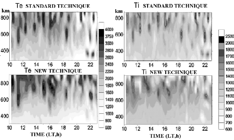
Figure 5: Electron and Ion temperatures during the November 15, 2001 experiment obtained with standard technique (top) and new technique (bottom).

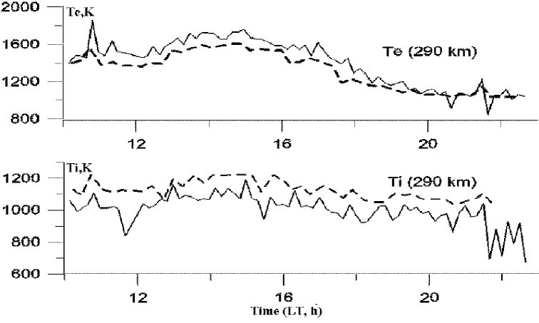
Figure 6: Electron and Ion temperatures during the November 15, 2001 experiment obtained with standard technique (solid line) and new technique (dashed line) at 290km.

6 Conclusion

A technique has been suggested for improving the spectral resolution in the case of the incoherent scattering when sounding by simple (squared) pulses. The method is based on an experimental model of single spectra of the scattered signal realizations. Furthermore, the model of a single realization spectrum represents a comb structure, the sum of delta-functions of a different amplitude at different frequencies convoluted with a certain function that is determined by the form of the sounding signal and of the receiving window. In terms of such an empirical model, it is possible to perform a deconvolution of the mean spectral power of the received signal with the smearing function in order to obtain the mean spectral power, at the stage of analysis of separate realizations, which is equivalent to an improvement of the spectral resolution of the method. Furthermore, the model parameters are derived by a simple determination of the positions and amplitudes of local maxima of the individual realizations spectra, which does not require much computer time and can be implemented in the real-time mode. Also, the technique does not require knowing the form of the ’smearing’ function and could therefore be used to improve the spectral resolution over a wide range of cases.

The proposed technique appears to be able to be extended also to other types of single backscattering from the ionosphere. As an example, Figure 7 illustrates the processing of experimental data on another type of singly backscattered signal from the ionosphere - backscattering from the E-layer irregularities elongated with the geomagnetic field. All curves in this case are similar to the curves in Figure 3 and, as in the case of Figure 3, there is a good agreement of $<|u_{teor}(\omega)|^{2}>$ to the spectrum $<|u(\omega)|^{2}>$ with the removal of the convolution with the smearing function $S(\omega)$.

So, the proposed technique of incoherent scattered signal processing (5,8) could be used in some cases for increasing the spectral resolution of the incoherent scattering method. But, to use this technique one needs good signal to noice ratio, and narrow enought spectral smoothing function to one could use approximation (8) which does not depend on spectral smoothing function $S(\omega)$, instead of accurate solution of (6).

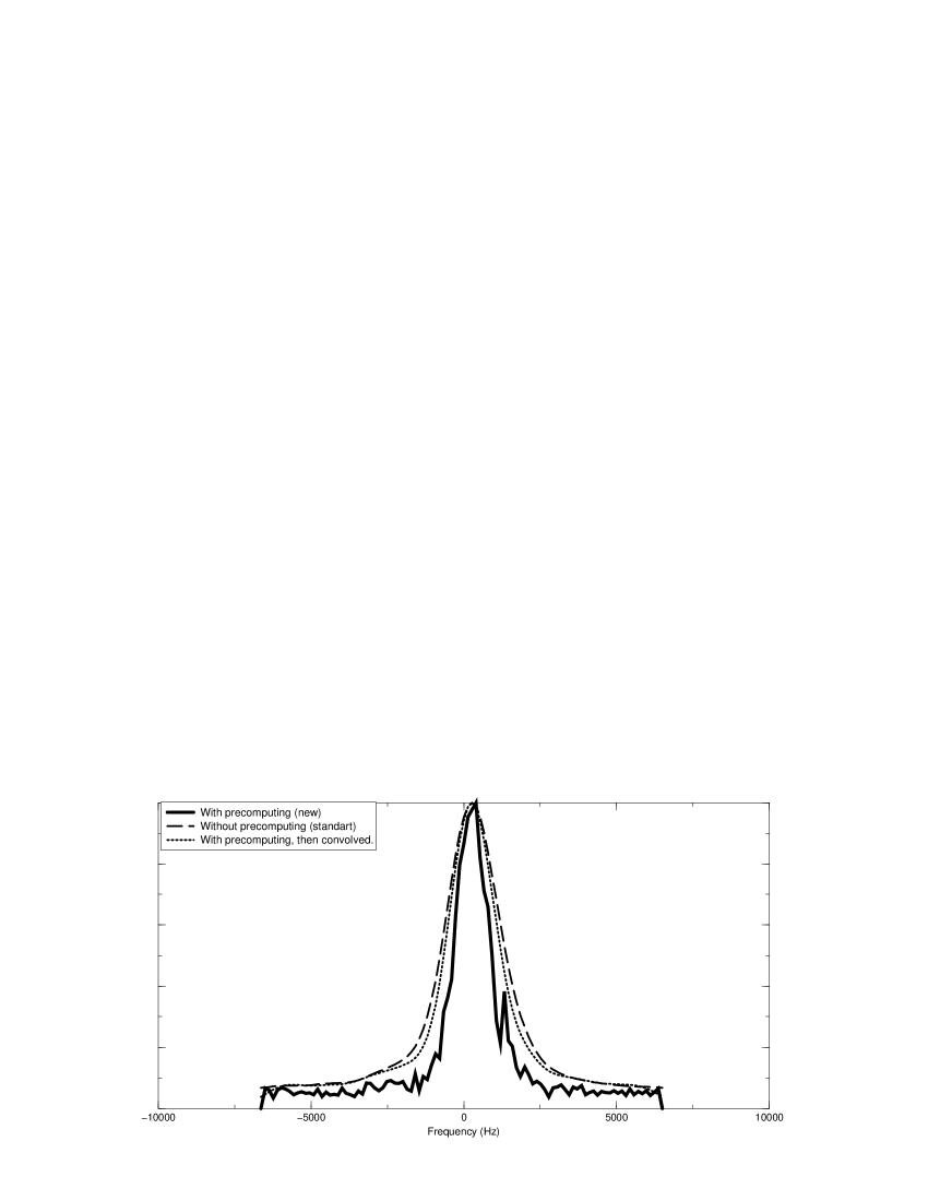
Figure 7: Mean spectral power of the backscattered signal from the E-layer irregularities elongated with the geomagnetic field (dashed line), mean deconvolved spectral power of the signal calculated by the proposed technique (thick solid line), and calculated by the proposed technique with a subsequent convolution with the spectral smearing function (dotted line). Accumulation - 1000 realizations.

References

- [Berngardt and Potekhin (2000)] Berngardt O.I. and Potekhin A.P., Radar equations in the radio wave backscattering problem, Radiophysics and Quantum electronics, 43(6), 484–492, 2000
- [Evans (1963)] Evans J.V., Theory and practice of ionosphere study by Thomson scatter radar, Proc.IEEE, 57, 496–530,1963
- [Farley (1972)] Farley D.T., Multiple-pulse incoherent scatter correlation function measurements, Radio Science, 7(6), 661–666, 1972
- [Holt et al. (1992)] Holt J.M., Rhoda D.A., Tetenbaum D., van Eyken A.P. Optimal analysis of incoherent scatter radar data, Radio Science, 27(3), 435–447, 1992
- [Lentinen (1986)] Lehtinen M.S., Statistical theory of incoherent scatter radar measurements, Ph.D.Thesis.- Univ. of Helsenki, -1986 -97p.
- [Shpynev (2000)] Shpynev B.G., Methods of Processing Incoherently Scattered Signals with the Fadaray Effect Taken Into Account., Ph.D.Thesis, Irkutsk, 2000, 142 p.(in Russian)
- [Sulzer (1993)] Sulzer M.P., A new type of alternating code for incoherent scatter measurements, Radio Science, 28, 995–1001, 1993