Contribution of forbidden orbits in the photoabsorption spectra of atoms and molecules in a magnetic field

Abstract

In a previous work [Phys. Rev. A 66, 0134XX (2002)] we noted a partial disagreement between quantum $R$-matrix and semiclassical calculations of photoabsorption spectra of molecules in a magnetic field. We show this disagreement is due to a non-vanishing contribution of processes which are forbidden according to the usual semiclassical formalism. Formulas to include these processes are obtained by using a refined stationary phase approximation. The resulting higher order in $\hbar$ contributions also account for previously unexplained “recurrences without closed-orbits”. Quantum and semiclassical photoabsorption spectra for Rydberg atoms and molecules in a magnetic field are calculated and compared to assess the validity of the first-order forbidden orbit contributions.

I Introduction

The photo-absorption spectrum of excited atoms or molecules placed in a magnetic field displays complex structures. Closed-orbit theory consists of a fully quantitative approach in which the large-scale structures of the spectra are explained in terms of classical trajectories closed at the nucleus, i.e., leaving and returning to the core. Each orbit produces on its return an oscillation in the photo-absorption cross-section; the Fourier-transform of the spectrum, known as the recurrence spectrum therefore exhibits sharp peaks at the period of the orbits. First developed for the hydrogen atom du delos88 , closed-orbit theory was then extended to treat the case of non-hydrogenic Rydberg atoms: the additional spectral modulations appear as the result of successive quantum encounters of the Rydberg electron with the core dando etal95 . The wave-function follows the hydrogenic classical orbits in the region where the Coulomb and the external fields compete (“outer region”), but near the core, where the external fields are negligible (“inner region”), the wave-function is described quantum-mechanically.

More recently, we proposed a closed-orbit theory treatment of molecules in external fields m&m01 ; mdm02 : in addition to elastic scattering, inelastic scattering gives rise to novel spectral modulations. The relative importance of elastic and inelastic scattering was shown to depend on the short-range phase-shifts, the molecular quantum defects. In the inelastic collision process, the molecular core undergoes a transition from its ground state to an excited state, and the dynamical regime of the Rydberg electron changes accordingly, say from a chaotic to a near integrable classical regime. Good quantitative agreements between quantum calculations and closed-orbit theory in the case of an external magnetic field were obtained. However we noted in Ref. mdm02 a discrepancy between the quantum and the semiclassical results for certain peaks of the recurrence spectrum. In general, disagreements between semiclassical and quantum recurrence spectra are due to higher order (in $\hbar$) effects such as bifurcations or ghost orbits, and specific formulas to account for these effects have been developed sadovskii delos96 ; main wunner97 . The discrepancies we observed in mdm02 are due to another type of effect, namely the manifestation of orbits which are forbidden to first order in $\hbar;$ these orbits are forbidden either i) because they should not be excited according to the usual semiclassical formalism or ii) because they do not classically exist.

We investigate in this work the effects of such first-order suppressed orbits. We will derive formulas for including their contribution in the recurrence spectra by going beyond the usual stationary phase approximation employed in the standard form of closed-orbit theory. The formulas will be tested versus exact quantum calculations for different model atomic and molecular systems in an external magnetic field. The two orbits that will be dealt with specifically are the orbit perpendicular to the field, which should not be excited when it lies in the node of a wavefunction, and the orbit parallel to the field, which does not exist classically when the electron’s angular momentum projection on the field axis $L_{z}$ is non-vanishing (since the Hamiltonian remains divergent on the $z$ axis even after regularization). The contribution of orbits lying in the node of a wave-function was first observed by Shaw et al. shaw etal95 when comparing quantum and semiclassical calculations for the diamagnetic hydrogen atom in the near-integrable regime (scaled energies $\epsilon\simeq-0.7$). They obtained a formula for including the first-order forbidden contribution of the perpendicular orbit, which appeared as a small feature in the recurrence spectra. In non-hydrogenic systems, we can expect the effects associated with “forbidden” orbits to be far more important than in hydrogen given that core-scattering mixes the contributions of different orbits. Moreover, although it may have been expected that at higher scaled energy the contribution of on-node orbits would become insignificant (as the classical amplitudes decrease), we will see that their inclusion is necessary to account for the correct amplitude in the modulations produced by orbits which have bifurcated from them. The existence of recurrences produced by “non-existing” orbits on the field axis was reported for Rydberg atoms in an electric field by Robicheaux and Shaw robicheaux shaw98 , who developed a heuristic formula which yielded a poor agreement between semiclassical and quantum calculations. We will derive a formula for appropriately taking into account such classically forbidden orbits and compare it to quantum calculations in the case of an external magnetic field. In passing we will also show that the contribution of the parallel orbit when it is allowed (i.e., for $L_{z}=0$) can be obtained by treating it as any other orbit, provided a higher order refined stationary phase integration is used (whereas the parallel orbit has always been treated as a special case, following the original derivation given by Gao and Delos gao delos92 ).

The paper is organized as follows. We recall in Sec. II the usual semiclassical formulas of closed-orbit theory (with provision for multichannel core scattering). Sec. III details the derivation of the contribution to the photoabsorption spectra of the first-order forbidden orbits. We report in Sec. IV quantum and semiclassical calculations for different values of the quantum defects, scaled energies or magnetic field ranges, focusing on the contribution of those forbidden orbits. We give our conclusions in Sec. V.

II Overview of standard multichannel closed-orbit theory

Closed-orbit theory explains the dynamics underlying the photoabsorption spectra of Rydberg atoms or molecules in external fields in terms of closed orbits: following initial photo-excitation, the wavefunction of the excited electron propagates first in a region near the ionic core (“inner region”), in which the external field can be neglected. Beyond the inner region, the wave-function is propagated semiclassically along classical trajectories. Some trajectories return to the inner region, and the semiclassical wavefunction carried by those trajectories is matched to an exact wavefunction in the inner region given by a standard (field-free) multichannel quantum defect theory (MQDT) expansion. The superposition of these returning waves with the initially dipole-excited wavefunction produces sinusoidal modulations in the photoabsoprtion spectrum, which appear as isolated peaks in the Fourier-transformed (“recurrence”) spectrum. Further modulations (i.e., peaks in the recurrence spectrum) are caused by the core-scattering process; in a multichannel problem, the electron can exchange energy and angular momenta with the core, so after the collision the electron wavefunction propagates outward again, and when it leaves the inner region the wavefunction will follow once again classical trajectories. If the collision was perfectly elastic, the electron will follow one of the previously followed trajectories; on the other hand, inelastic collisions will result in trajectories pertaining to a different classical regime.

In Ref. mdm02 we described in detail photoabsorption from a ground state diatomic molecule in a static magnetic field. After photoexcitation, the molecular core could either be rotationally excited ($N=2$) or non-excited $(N=0,$ where $N$ is the core angular momentum). The molecular core then plays the role of an effective 2-level scatterer which combines classical trajectories belonging to 2 different dynamical regimes (typically, chaotic and near-integrable regimes), thereby producing additional modulations in the photoabsorption spectrum. The way these combinations occur depends both on the classical characteristics (amplitude $A_{k}$ and action $S_{k}$ of the $k$th trajectory), and on the properties of the scatterer (which is given by the scattering transition matrix, $T$). Scaled energy spectroscopy consists of simultaneously varying the magnetic field strength $\gamma$ and the laser excitation frequency so as to keep $\epsilon=E\gamma^{-2/3}$ constant, where $E$ is the energy of the Rydberg electron; $\epsilon$ is the scaled energy, which depends on the core state $j$ through the energy partition between the core and the outer electron. Although scaling for molecules is only approximate, we have seen in mdm02 how a molecular system can be scaled conveniently; $\hbar_{\textrm{eff}}$ will stand for $\gamma^{1/3},$ since the field strength plays the rôle of the Planck constant friedrich wintgen89 . The absorption rate in the one core-scatter approximation is then given by [see Eq. (3.30) in mdm02 ]

$$\mathcal{F}(\hbar_{\text{eff}})=2^{19/4}\pi^{3/2}\sum_{j}\sum_{\alpha}\sum_{\alpha^{\prime}}\operatorname{Im}\left\{\left\langle\alpha\right|\left.j\right\rangle\rm{C}_{\alpha}\rm{C}_{\alpha^{\prime}}e^{i\pi\left(\mu_{\alpha}+\mu_{\alpha^{\prime}}\right)}\right.$$

$$\left.\left[\left\langle j\right|\left.\alpha^{\prime}\right\rangle\sum_{k}\tilde{\mathcal{R}}_{k}^{j}(\epsilon_{j})+\hbar_{\text{eff}}^{1/2}2^{11/4}\pi^{3/2}\sum_{j^{\prime}}\left\langle j^{\prime}\right|\left.\alpha^{\prime}\right\rangle T_{jj^{\prime}}\sum_{k}\tilde{\mathcal{R}}_{k}^{j^{\prime}}(\epsilon_{j^{\prime}})\sum_{q}\tilde{\mathcal{R}}_{q}^{j}(\epsilon_{j})\right]\right\}.$$ (1)

The notation has been completely detailed in Sec. III of mdm02 , but in short: $j$ (and $j^{\prime}$) is a compound index accounting for the core-electron couplings when the electron dynamics has uncoupled from the core. If we assume H₂ as the prototype molecule, the initial state has the quantum numbers $J=0,$ $l=0$ ($J$ is the total angular momentum, $l$ the orbital momentum of the outer electron), the sum over $j$ runs over the core states $N=0,$ $M_{N}=M$ and $N=2,$ $M_{N}=M-1,M,M+1$ where $M_{N}$ is the projection of $N$ on the field axis; $M,$ the projection of the total angular momentum on the field axis, is the only quantum number conserved throughout the entire physical process. $\alpha$ gives the set of quantum numbers in the molecular frame, when the electron is coupled to the molecular axis; the sum runs here on $\Lambda=0$ ($\Sigma$ state) and $\Lambda=1$ ($\Pi$ state); $\mu_{\Sigma}$ and $\mu_{\Pi}$ are the corresponding short-range molecular quantum defects. $\rm{C}_{\alpha}$ is a coefficient giving the relative strength of the electronic dipole transition amplitudes; from the united dipole approximation, known to be valid for H${}_{2},$ we have $\rm{C}_{\Sigma}=1$ and $\rm{C}_{\Pi}=\sqrt{2}.$ $\left\langle j\right|\left.\alpha\right\rangle$ are the transformation coefficients between the molecular and the uncoupled frames. The elements of the scattering matrix $T_{jj^{\prime}}$ depend solely upon the quantum defects and the $\left\langle j\right|\left.\alpha\right\rangle$ elements. The quantities $\tilde{\mathcal{R}}_{k}^{j}(\epsilon_{j})$ are the only ones that depend on the classical properties of the Rydberg electron trajectories. We have, for the trajectory $k$ associated with the core in state $j$ [Eqs. (3.18) and (D1) of mdm02 ]:

$$\tilde{\mathcal{R}}_{k}^{j}(\epsilon_{j})=\left|\sin\theta_{ik}\sin\theta_{fk}\right|^{1/2}\sum_{l_{j}l_{j^{\prime}}}(-1)^{l_{j}+l_{j^{\prime}}}Y_{l_{j^{\prime}}m_{j^{\prime}}}(\theta_{ik})Y_{l_{j}m_{j}}^{\ast}(\theta_{fk})$$

$$\tilde{r}_{f}^{-1/4}A_{k}^{N_{j}m_{j}}(r_{f},\theta_{fk})e^{i\left(2\pi\tilde{S}_{k}^{N_{j}m_{j}}/\hbar_{\text{eff}}-\omega_{k}^{N_{j}m_{j}}\pi/2-3\pi/4\right)},$$ (2)

where $l_{j},l_{j^{\prime}}\geqslant\left|m_{j}\right|$ and $m_{j^{\prime}}=m_{j}$. $\theta_{ik}$ and $\theta_{fk}$ are the initial and final angles of the $k$th trajectory relative to the magnetic field direction, which is taken to be along the $z$ axis. $A_{k}^{N_{j}m_{j}}$ and $\tilde{S}_{k}^{N_{j}m_{j}}$ are the scaled classical amplitude and action, evaluated at the corresponding scaled energy $\epsilon_{j}$; $\omega_{k}^{N_{j}m_{j}}$ is the associated Maslov index. $Y_{l_{j}m_{j}}(\theta_{ik})$ will be used throughout as a short-hand notation for $Y_{l_{j}m_{j}}(\theta_{ik},0),$ since the conserved axial symmetry has been separated from the 2-dimensional semiclassical problem; we have accordingly used a different notation for the quantized value of the Rydberg electron’s angular momentum projection $m$ and its classical counterpart $L_{z}$ appearing in the two-dimensional diamagnetic Hamiltonian. Equation (2) must be modified for orbits lying along the magnetic field axis ($\theta_{ik}=\theta_{fk}=0$) as detailed below. Note that Eq. (1) is also valid for ground state hydrogen photoexcited to odd-parity states (by setting $\mu_{\Sigma}$ and $\mu_{\Pi}$ to zero; then the $T$ matrix vanishes) as well as for non-hydrogenic Rydberg atoms with a single quantum defect $\mu_{l=1}$ (by setting $\mu_{\Sigma}=\mu_{\Pi}=\mu_{l=1}$; the $T$ matrix is then diagonal).

Eqs. (1) and (2) are obtained by matching the semiclassical wavefunction $\psi_{SC}^{N_{j}m_{j}}$ associated with the core in state $\left|N_{j}m_{j}\right\rangle$ which returns to the core region to a MQDT expansion on a boundary circle $(r_{f},\theta_{f})$. The semiclassical wavefunction reads

$$\psi_{SC}^{N_{j}m_{j}}(r_{f},\theta_{f})=\sum_{k}\psi_{\mathrm{out}}^{N_{j}m_{j}}(r_{i},\theta_{ik})\left|\frac{r_{i}^{2}\sin\theta_{ik}}{r_{f}^{2}\sin\theta_{f}}\right|^{1/2}A_{k}^{N_{j}m_{j}}(r_{f},\theta_{f})\exp i\left(S_{k}^{N_{j}m_{j}}(r_{f},\theta_{f})-\omega_{k}^{N_{j}m_{j}}\pi/2\right),$$ (3)

where $\psi_{\mathrm{out}}^{N_{j}m_{j}}(r_{i},\theta_{ik})$ represents the initially outgoing waves, which were propagated semiclassically beyond the boundary $(r_{i},\theta_{i}).$ We shall write $\psi_{\mathrm{out}}^{N_{j}m_{j}}(r_{i},\theta_{ik})$ as

$$\psi_{\mathrm{out}}^{N_{j}m_{j}}(r_{i},\theta_{ik})=\sum_{l_{j}\geqslant\left|m_{j}\right|}\mathcal{Q}_{l_{j}}Y_{l_{j}m_{j}}(\theta_{ik}),$$ (4)

with

$$\mathcal{Q}_{l_{j}}=-i\pi^{1/2}2^{3/4}r_{i}^{-3/4}(-1)^{l_{j}}e^{i\left(\sqrt{8r_{i}}-3\pi/4\right)}\sum_{\alpha}e^{i\pi\mu_{\alpha}}\left\langle N_{j}l_{j}m_{j}\right|\left.\alpha\right\rangle D_{\alpha},$$ (5)

where the $D_{\alpha}$ are the dipole transition amplitudes in the molecular frame. The MQDT expansion reads in the uncoupled basis

$$\psi_{\mathrm{qdt}}(r_{f})=\sum_{j}\left|j\right\rangle\sum_{j^{\prime}}c_{j^{\prime}}\left[\delta_{jj^{\prime}}f_{l_{j}}(r_{f})+T_{jj^{\prime}}g_{l_{j}}^{+}(r_{f})\right],$$ (6)

where $f$ and $g^{+}$ are Coulomb functions ($f$ is regular at the origin, $g^{+}$ is an outgoing wave). The expansion coefficients $c_{j^{\prime}}$ are obtained by matching Eqs. (3) and (6) on the boundary. The matching condition reads

$$c_{j}g_{l_{j}}^{-}(r_{f})/2i=-2\pi\int_{0}^{\pi}d\theta_{f}\,\sin\theta_{f}Y_{l_{j}m_{j}}^{\ast}(\theta_{f})\psi^{N_{j}m_{j}}(r_{f},\theta_{f});$$ (7)

the integral is performed for each trajectory $k$ in the stationary phase approximation, since the phase is stationary along the final angle of the trajectory $\theta_{fk}$ hupper etal96 . The value of the coefficients $c_{j}$ are then inserted in the expression giving the dipole transition amplitudes, of the form $\left\langle\psi_{0}\right|\mathbf{D}\left|\psi_{\mathrm{qdt}}\right\rangle$ where $\left|\psi_{0}\right\rangle$ is the initial state prior to photoabsorption. The formulas for the oscillator strength and the absorption rate are then obtained. Obviously when Eqs. (3) or (7) vanish, e.g., $Y_{l_{j}m_{j}}(\theta_{ik})=0$ or $Y_{l_{j}m_{j}}^{\ast}(\theta_{f})=0$, then $\tilde{\mathcal{R}}_{k}^{j}(\epsilon_{j})$ vanishes, and these orbits should not produce modulations in the oscillator strength.

III Contribution of first-order forbidden orbits

III.1 General remarks

Although Eqs. (1) and (2) predict that if $\tilde{\mathcal{R}}_{k}^{j}(\epsilon_{j})$ vanishes, the orbit $k$ should not contribute to the recurrence spectrum, we had observed in mdm02 a mismatch between semiclassical and quantum classical calculations for molecules in fields in the amplitude of certain peaks in the recurrence spectrum. This mismatch was interpreted as arising from the interference of the orbit perpendicular to the field (which lies on the node of a spherical harmonic when $M=0$ and is thus semiclassically forbidden) with the $R_{2}^{1}$ “pac-man” orbit. As stated, the recurrences associated with classical orbits lying in the node of a wavefunction were first observed by Shaw et al. shaw etal95 when comparing quantum and semiclassical calculations for the diamagnetic hydrogen atom at low scaled energies ($\epsilon\simeq-0.7$). They obtained a formula for the contribution of the perpendicular orbit by matching the returning semiclassical wave to an “ansatz” (a rotated first order Bessel function). In this section we shall derive simply the contribution to the oscillator strength of this type of first-order suppressed orbit by employing the same framework introduced in Sec. II, without introducing additional assumptions; only the stationary phase integration needs to be performed differently. We will also derive a formula to account for the peaks in the $m=1$ recurrence spectra appearing at the scaled action of the $m=0$ parallel orbit, since the parallel orbit does not exist classically when $L_{z}\neq 0$ and there is therefore no corresponding $\tilde{\mathcal{R}}_{k}^{j}(\epsilon_{j})$ factor. Numerical results and examples will be given in Sec. IV.

III.2 Contribution of on-node suppressed orbits

The rationale for including the contribution of orbits lying on the node of a wavefunction was already given in shaw etal95 : strictly speaking, an orbit $k$ closed at the core with initial and returning angles $\theta_{ik}$ and $\theta_{fk}$ is not isolated, but has neighboring orbits which are not closed at the origin. We assume a neighboring orbit returns with an angle $\bar{\theta}_{f}$ and envisage the initial angle $\bar{\theta}_{i}$ of this orbit to be a function of $\bar{\theta}_{f},$ i.e., $\bar{\theta}_{i}=\theta(\bar{\theta}_{f})$. To first order in $\bar{\theta}_{f}-\theta_{fk}$ we have

$$Y_{l_{j}m_{j}}(\bar{\theta}_{i}) =Y_{l_{j}m_{j}}(\theta_{ik})+\frac{\partial Y_{l_{j}m_{j}}(\theta_{ik})}{\partial\theta_{ik}}\left.\frac{\partial\theta_{ik}}{\partial\bar{\theta}_{f}}\right|_{\theta_{fk}}\left(\bar{\theta}_{f}-\theta_{fk}\right)$$ (8)

$$Y_{l_{j}m_{j}}^{\ast}(\bar{\theta}_{f}) =Y_{l_{j}m_{j}}^{\ast}(\theta_{fk})+\left.\frac{\partial Y_{l_{j}m_{j}}^{\ast}(\bar{\theta}_{f})}{\partial\bar{\theta}_{f}}\right|_{\theta_{fk}}\left(\bar{\theta}_{f}-\theta_{fk}\right)$$ (9)

In the usual case, the contribution of the neighboring orbits with initial and final angles $(\bar{\theta}_{i},\bar{\theta}_{f})$ is negligible when compared to the central orbit with angles $(\theta_{ik},\theta_{fk})$. However, when the central orbit lies on a node of a spherical harmonic, the semiclassical wave-function can only be carried by the neighboring orbits, and this contribution can be significant provided the classical density of trajectories is sufficiently large on return to the core.

It turns out that, to first order in $\bar{\theta}_{f}-\theta_{fk}$, such a contribution comes into play if we have both $Y_{l_{j}m_{j}}(\theta_{ik})=0$ and $Y_{l_{j}m_{j}}^{\ast}(\theta_{fk})=0$. If $k$ is such an orbit, its contribution to the outgoing wave $\psi_{\mathrm{out}}^{N_{j}m_{j}}$ [Eq. (4)] vanishes. The contribution of the neighboring orbits are taken into account by inserting Eq. (8) in Eq. (4) and Eq. (9) in Eq. (7); the right hand-side of Eq. (7) then takes the form:

$$-2\pi\int_{0}^{\pi}d\bar{\theta}_{f}\left|\sin\bar{\theta}_{f}\sin\theta_{ik}\right|^{1/2}\sum_{l_{j^{\prime}}}\mathcal{Q}_{l_{j^{\prime}}}\frac{\partial Y_{l_{j^{\prime}}m_{j}}(\theta_{ik})}{\partial\theta_{ik}}\left.\frac{\partial\theta_{ik}}{\partial\bar{\theta}_{f}}\right|_{\theta_{fk}}\left.\frac{\partial Y_{l_{j}m_{j}}^{\ast}(\bar{\theta}_{f})}{\partial\bar{\theta}_{f}}\right|_{\theta_{fk}}$$

$$A_{k}^{N_{j}m_{j}}(r_{f},\bar{\theta}_{f})\left[\left(\bar{\theta}_{f}-\theta_{fk}\right)^{2}\exp i\left(S_{k}^{N_{j}m_{j}}(r_{f},\bar{\theta}_{f})-\omega_{k}^{N_{j}m_{j}}\pi/2\right)\right].$$ (10)

Following Hüpper et al. hupper etal96 , we express the action on the boundary $(r_{f},\bar{\theta}_{f})$ in terms of the action of the orbit closed at the origin, $S_{k}^{N_{j}m_{j}}(r_{f},\bar{\theta}_{f})\simeq S_{k\mathrm{(closed)}}^{N_{j}m_{j}}+\sqrt{r_{f}/8}\left(\bar{\theta}_{f}-\theta_{fk}\right)^{2}$. The integral can now be performed; a straightforward stationary phase integration would lead to zero, since the integrand vanishes at the point of stationary phase $\bar{\theta}_{f}=\theta_{fk}$. However, we can assume the integrand to vary slowly around the angle of stationary phase, and integrate exactly the term between square brackets (see Appendix A). In the semiclassical limit, Eq. (21) is appropriate. Eq. (10) then becomes

$$\hbar e^{i\pi/2}2^{1/2}\left[r_{f}^{-1/4}A_{k}^{N_{j}m_{j}}(r_{f},\theta_{fk})\right]^{2}\mathrm{sgn}(\frac{\partial\theta_{ik}}{\partial{\theta}_{fk}})$$

$$\left\{-2^{3/4}\pi\left(2\pi\hbar\right)^{1/2}e^{i\pi/4}\sum_{l_{j^{\prime}}}\mathcal{Q}_{l_{j^{\prime}}}\frac{\partial Y_{l_{j^{\prime}}m_{j}}(\theta_{ik})}{\partial\theta_{ik}}\left.\frac{\partial Y_{l_{j}m_{j}}^{\ast}(\bar{\theta}_{f})}{\partial\bar{\theta}_{f}}\right|_{\theta_{fk}}\right.$$

$$\left.\left|\sin\theta_{ik}\sin\theta_{fk}\right|^{1/2}r_{f}^{-1/4}A_{k}^{N_{j}m_{j}}(r_{f},\theta_{fk})\exp\left[i\left(S_{k\mathrm{(closed)}}^{N_{j}m_{j}}-2\sqrt{8r_{f}}-\omega_{k}^{N_{j}m_{j}}\pi/2\right)\right]\right\},$$ (11)

where we have used $A_{k}^{N_{j}m_{j}}(r_{f},\theta_{fk})=\left|\frac{\partial\theta_{ik}}{\partial{\theta}_{fk}}\right|^{1/2}$. For clarity we have singled out the factor specific to on-node orbits (in front of the curly brackets) relative to the expression valid for “typical” allowed orbits (inside the curly brackets). In particular it can be seen on-node orbits are suppressed by a factor $\hbar$ relative to typical orbits.

The relevant scaled factor $\tilde{\mathcal{R}}_{k\mathrm{-node}}^{j}(\epsilon_{j})$ giving the contribution of an orbit lying on the node of a wavefunction in the absorption rate is thus

$$\tilde{\mathcal{R}}_{k\mathrm{-node}}^{j}(\epsilon_{j}) =\hbar_{\textrm{eff}}2^{1/2}\mathrm{sgn}(\frac{\partial\theta_{ik}}{\partial{\theta}_{fk}})\left|\sin\theta_{ik}\sin\theta_{fk}\right|^{1/2}\sum_{l_{j}l_{j^{\prime}}}(-1)^{l_{j}+l_{j^{\prime}}}\frac{\partial Y_{l_{j^{\prime}}m_{j}}(\theta_{ik})}{\partial\theta_{ik}}\left.\frac{\partial Y_{l_{j}m_{j}}^{\ast}(\bar{\theta}_{f})}{\partial\bar{\theta}_{f}}\right|_{\theta_{fk}}$$

$$\left[\tilde{r}_{f}^{-1/4}A_{k}^{N_{j}m_{j}}(r_{f},\theta_{fk})\right]^{3}\exp i\left(2\pi\tilde{S}_{k}^{N_{j}m_{j}}/\hbar_{\textrm{eff}}-\omega_{k}^{N_{j}m_{j}}\pi/2-\pi/4\right).$$ (12)

This formula holds for non-vanishing angles. Specializing to our atomic and molecular model described above, we have $l=1,$ so this formula only applies to the orbit perpendicular to the field ($\theta_{ik}=\theta_{fk}=\pi/2$) for the $m=0$ manifolds (e.g., for a molecule, when $M=0,$ for an outer electron associated with core states having a projection $M_{N}=0$). Note that in the absence of core-effects, Eq. (10) becomes strictly equivalent to the correction obtained in shaw etal95 for the hydrogen atom.

III.3 Contribution of the “classically non-existing” parallel orbit

III.3.1 Contribution of the parallel orbit when $L_{z}=0$

We first recall that the orbit parallel to the field ($\theta_{ik}=\theta_{fk}=0)$ classically exists if $L_{z}=0$. Even then, this orbit is treated as a special case, because the formulas valid for the other orbits, Eqs. (1) and (2), need to be modified. This modification was originally obtained by matching the semiclassical returning wave to a particular Bessel function on the $z$ axis gao delos92 . We show here that the reason this orbit is “special” is that the standard stationary phase approximation vanishes. Indeed, setting $\left|\sin\theta_{ik}/\sin\theta_{fk}\right|^{1/2}\rightarrow\left|\partial\theta_{ik}/\partial\theta_{fk}\right|^{1/2}$ in the outgoing wave (3), the expression to be integrated arising from the matching condition Eq. (7) is

$$\int_{0}^{\pi}d\bar{\theta}_{f}\sin\bar{\theta}_{f}\exp(i\sqrt{r_{f}/8}\bar{\theta}_{f}^{2}/\hbar),$$ (13)

which is zero in the standard stationary phase approximation. However, an approximate closed form may be obtained (see Appendix B). To first order in $\hbar$, we have

$$\int_{0}^{\pi}d\bar{\theta}_{f}\sin\bar{\theta}_{f}\exp(i\sqrt{r_{f}/8}\bar{\theta}_{f}^{2}/\hbar)\approx\hbar e^{i\pi/2}\sqrt{2/r}.$$ (14)

This result is reduced by a factor $h^{1/2}e^{i\pi/4}2^{-1/4}\pi^{-1/2}$ relative to the standard stationary phase integration for non-zero degree orbits, which is exactly the result obtained in gao delos92 . The parallel orbit thus appears as a first-order suppressed orbit, which is apparent from its $\hbar$-dependence.

Figure 1: Recurrence spectrum (Fourier transform of the photoabsorption spectrum) for a non-hydrogenic atom with $\mu_{l=1}=0.5,$ $M=0,$ at $\epsilon=-0.7$, in the range $\gamma^{-1/3}=[60,120]$. Top: quantum calculations. Bottom: standard semiclassical calculations (solid line), semiclassical calculation including the higher-order contribution from the on-node orbit (broken line).

III.3.2 Contribution of the parallel orbit when $L_{z}\neq 0$

When $L_{z}$ is non-vanishing the diamagnetic Hamiltonian contains the repulsive term proportional to $\tilde{L}_{z}^{2}/\tilde{\rho}^{2}$, where $\tilde{L}_{z}=\gamma^{1/3}L_{z}$ is the scaled angular momentum and $\tilde{\rho}=\gamma^{2/3}\rho$ the scaled distance from the $z$ axis friedrich wintgen89 . Even though in the semiclassical limit $\tilde{L}_{z}$ is small (since $h_{\mathrm{\textrm{eff}}}\equiv\gamma^{1/3}\rightarrow 0$), the centrifugal term is infinite on the $z$ axis, and the parallel orbit no longer exists schweizer etal93 . However, we may expect orbits neighboring the $z$ axis and not closed at the nucleus to contribute to the oscillator strength, in the same manner as for the on-node orbit (orbits near the $z$ axis for $L_{z}\neq 0$ and their structural stability as $L_{z}\rightarrow 0$ where actually investigated in schweizer etal93 ). Starting from Eqs. (8) and (9) and setting $\left|\sin\theta_{ik}/\sin\theta_{fk}\right|^{1/2}\rightarrow\left|\partial\theta_{ik}/\partial\theta_{fk}\right|^{1/2}$ in Eq. (3) as in Sec. III.2 leads, after matching the semiclassical returning wave to the MQDT expansion, to the integral

$$\int_{0}^{\pi}d\bar{\theta}_{f}\sin\bar{\theta}_{f}\bar{\theta}_{f}^{2}\exp(i\sqrt{r_{f}/8}\bar{\theta}_{f}^{2}/\hbar).$$ (15)

To lowest order in $\hbar,$ we have (see Appendix B)

$$\int_{0}^{\pi}d\bar{\theta}_{f}\sin\bar{\theta}_{f}\bar{\theta}_{f}^{2}\exp(i\sqrt{r_{f}/8}\bar{\theta}_{f}^{2}/\hbar)\approx\frac{-4\hbar^{2}}{r}.$$ (16)

The resulting scaled contribution to the oscillator strength is given by

$$\tilde{\mathcal{R}}_{k\mathrm{-forb\,0}}^{j}(\epsilon_{j})=\hbar_{\textrm{eff}}^{3/2}2^{5/4}\pi^{-1/2}\mathrm{sgn}(\frac{\partial\theta_{ik}}{\partial{\theta}_{fk}})\sum_{l_{j}l_{j^{\prime}}}(-1)^{l_{j}+l_{j^{\prime}}}$$

$$\frac{\partial Y_{l_{j^{\prime}}m_{j}}(\theta_{ik})}{\partial\theta_{ik}}\left.\frac{\partial Y_{l_{j}m_{j}}^{\ast}(\bar{\theta}_{f})}{\partial\bar{\theta}_{f}}\right|_{\theta_{fk}}\left[\tilde{r}_{f}^{-1/2}A_{k}^{N_{j}m_{j}}(r_{f},\theta_{fk}=0)\right]^{2}$$

$$\exp i\left(2\pi\tilde{S}_{k}^{N_{j}m_{j}}/\hbar_{\textrm{eff}}-\omega_{k}^{N_{j}m_{j}}\pi/2\right).$$ (17)

Within our molecular model, this correction applies when $\left|m\right|=1$; this is of course the case when $M=1$, but even for $M=0,$ the outer electron may be associated with core states having a projection $\left|M_{N}\right|=1$, i.e., $N=2$ $M_{N}=1,-1$. Note that we have followed the by now standard notation whereby the zero-degree orbit amplitude is set as $A_{k}^{N_{j}m_{j}}(r_{f},\theta_{fk}=0)=\left|\partial\theta_{ik}/\partial\theta_{fk}\right|$ (although stricto sensu this is the square of the genuine two-dimensional semiclassical amplitude), so that now $\tilde{r}_{f}^{-1/2}A_{k}^{N_{j}m_{j}}(r_{f},\theta_{fk}=0)$ is independent of the boundary radius $r_{f}$.

III.4 $\hbar$ dependence

Unsurprisingly, the contribution of the forbidden orbits in the recurrence spectra have a different $\hbar$ dependence. The on-node orbit is suppressed by a factor $\hbar$ relative to a typical primitive orbit; the parallel orbit is suppressed by a factor $\hbar^{1/2}$ relative to a typical orbit, and the forbidden parallel by a factor $\hbar$ relative to the classically allowed parallel orbit and $\hbar^{3/2}$ relative to a typical orbit. This is to be contrasted with the core-scattered (“diffractive”) orbits: each encounter with the core brings in for a typical orbit a factor $\hbar^{1/2}$. Thus single core-scattering is expected to dominate the photoabsorption spectrum in the semiclassical regime; however, the $\hbar$ dependence is balanced by the amplitude factors, explaining why for individual orbits the forbidden contribution may be strong, as will be seen below. It may also be noted that the combination of orbits having different individual $\hbar$ dependence through core-scattering [last term in Eq. (1)] will give rise to peaks in the recurrence spectra with a dependence of the form $\hbar^{\nu/2}$, where $\nu$ is an integer depending on the type of primitive orbits connected by the core-scattering process. In particular, core-scattering between two forbidden parallel orbits is expected to be highly suppressed in the semiclassical limit.

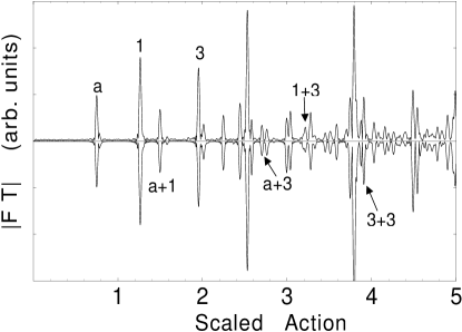
Figure 2: General view of the recurrence spectrum for a molecule with the set of quantum defects $\mu_{\Sigma}=-0.3,$ $\mu_{\Pi}=0.1,$ $M=0$, at $\epsilon_{N=0}=-0.3$ and $\epsilon_{N=2}=-0.8$ in the range $\gamma^{-1/3}=[60,120]$. The semiclassical result (bottom) has been calculated in the one core-scatter approximation, but the first-order suppressed contributions have been included.

IV Results

We compare below quantum and semiclassical calculations to assess the importance of the forbidden orbits in the recurrence spectra of atoms and molecules. The numerical examples given in this section correspond to non-hydrogenic atoms and different molecules obtained by choosing different sets of quantum defects, within the framework of the model described in Sec. II.

Fig. 1 displays the recurrence spectrum of a non-hydrogenic atom with $\mu_{l=1}=0.5,$ $M=0,$ at $\epsilon=-0.7$, in the range $\gamma^{-1/3}=[60,120]$. The top figure gives the quantum calculation, whereas the solid line in the bottom part of the plot results from the standard semiclassical treatment; this solid line only accounts for less than half of the peaks in the recurrence spectrum. The missing peaks relative to the quantum results arise from the orbit $R_{1}$ perpendicular to the field (and its $n$th repetition $R_{n}$) — which lies on the node of the wavefunction and is thus not excited according to the standard treatment — as well as from the combinations produced by core-scattering between $R_{n}$ and the parallel orbit and between the on-node orbits. The broken line includes the contribution of the on-node orbit [Eq. (12)] in the semiclassical calculation.

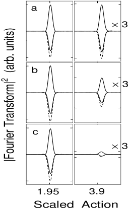
Figure 3: Recurrence spectra for non-hydrogenic atoms with $\mu_{l=1}=0.5$ [a], $\mu_{l=1}=0.25$ [b] and $\mu_{l=1}=0.1$ [c]. The left panel represents the peak labelled $3$ in Fig. 2, the right panel shows the combination peak $1+3$ (the amplitude of the $1+3$ peak has been multiplied by 3 relative to the amplitude of the peak on the left panel). For each peak, the quantum result (top) is plotted versus semiclassical calculations (upside-down) without (solid line) and with (broken line) the higher order contributions.

At higher scaled energies, the contribution of the forbidden $R_{n}$ orbit is visible through the mismatch observed in mdm02 between the height of the peaks in the quantum and semiclassical recurrence spectra. Fig. 2 displays a global view of the recurrence spectrum for a molecule with the set of quantum defects $\mu_{\Sigma}=-0.3,$ $\mu_{\Pi}=0.1,$ $M=0$, at $\epsilon_{N=0}=-0.3$ and $\epsilon_{N=2}=-0.8$ in the range $\gamma^{-1/3}=[60,120]$. These quantum defects yield a balanced contribution of the different type of orbits: the primitive geometric orbits (that is the orbits that appear in the recurrence spectrum of the hydrogen atom), the elastic scattered diffractive orbits (that appear in the recurrence spectra of non-hydrogenic atoms and in molecules) and the inelastic scattered diffractive orbits (that solely appear in molecular systems). In Figs. 3–5, we zoom on some individual peaks in the recurrence spectra, choosing different sets of quantum defects but keeping the other parameters (scaled energies, $\gamma$ range) constant, to observe the presence of the on-node orbit and how its interplay with core-scattering affects the amplitude of the recurrence peaks.

Fig. 3 displays the recurrence spectra for non-hydrogenic atoms with $\mu_{l=1}=0.5$ [a], $\mu_{l=1}=0.25$ [b] and $\mu_{l=1}=0.1$ [c], at $\epsilon=-0.3$, around the peaks labelled $3$ and $1+3$ in Fig. 2. According to the standard treatment (solid line), peak $3$ is produced by the $R_{2}^{1}$ “pac-man” orbit (the shapes and characteristics of the orbits mentioned here are given in Table I and Fig. 6 of mdm02 ; $R_{2}^{1}$ has bifurcated from $R_{2}$ at a slightly lower energy, and thus the two orbits have nearly the same scaled action), and $1+3$ results from the combination of the $V_{1}^{1}$ “balloon” orbit (peak $1$) and $R_{2}^{1}$ through core-scattering. The mismatch for the peak $3$ arises from interference between the contributions of the $R_{2}^{1}$ and the on-node $R_{2}$ orbit; indeed, including the on-node orbit in the semiclassical calculations results in excellent agreement with the quantum result. The peak $3$ thus results from the interference of primitive orbits and accordingly does not depend on the value of the quantum defect; however the peak $1+3$ does depend on the quantum defect and vanishes in the limit $\mu_{l=1}\rightarrow 0$; the contribution of the on-node orbit in $1+3$ is seen to be important (in absolute terms) only provided the quantum defect is large. Note that in principle we should also have taken into account the first and third repetitions of the perpendicular orbit, but their corresponding amplitudes are very small, so these orbits have a negligible contribution to the recurrence spectra.

The situation depicted in Fig. 4 is more involved: a close up of the peak at $\tilde{S}=3.9$ (labelled $3+3$ in Fig. 2) is shown for a molecule with quantum defects $\mu_{\Sigma}=0.5,$ $\mu_{\Pi}=0$ [a] and $\mu_{\Sigma}=0.5,$ $\mu_{\Pi}=0.5$ [b]; the peak $3+3$ arises from recurrences produced by different orbits: the second return of $R_{2}^{1}$ and the fourth return $R_{4}$ of the on-node perpendicular orbit, the combinations $R_{2}^{1}+R_{2}^{1}$, $R_{2}^{1}+R_{2}$ and $R_{2}+R_{2}$ via core-scattering. The resulting peak amplitude depends both on the quantum defects (which rule the core-scattering amplitudes) and on the inclusion of the two on-node orbits: in the first case the standard semiclassical result underestimates the exact quantum calculation, whereas in Fig. 4 (b) the standard semiclassical result overestimates the correct recurrence strength. Adding the contribution of the on-node orbits in the semiclassical treatment results in both cases in a better agreement with the quantum calculations.

Fig. 5 displays the peak labelled $\mathrm{a}+3$ in Fig. 2 but for the choice of quantum defects $\mu_{\Sigma}=0.5,$ $\mu_{\Pi}=0$. This peak results from the inelastic scattering between $R_{2}^{1}$ at $\epsilon=-0.3$ and the perpendicular orbit associated with the core state $N=2,$ $m=\pm 1$ at $\epsilon=-0.8.$ Again, the standard closed-orbit result underestimates the recurrence strength and the inclusion of the first-order suppressed on-node orbit improves the agreement with the quantum results.

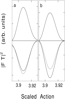
Figure 4: The peak labelled $3+3$ in Fig. 2 is shown for a molecule with quantum defects $\mu_{\Sigma}=0.5,$ $\mu_{\Pi}=0$ [a] and $\mu_{\Sigma}=0.5,$ $\mu_{\Pi}=0.5$ [b]. The inclusion of the higher order contributions (broken line) gives a better agreement with the quantum calculations (top) than the standard semiclassical formalism (solid line upside-down).

Finally, Fig. 6 shows a portion of the recurrence spectrum for the hydrogen atom at $\epsilon=-0.55,$ $M=1,$ in the range $\gamma^{-1/3}=[30,240]$. We have zoomed the peaks at $\tilde{S}=0.95$ and $\tilde{S}=1.91$ which are due to the first and second returns of the classically “non-existing” forbidden parallel orbit. Note that the peak at $\tilde{S}=0.95$ sits on the right shoulder of the much stronger $R_{1}$ orbit, whereas the second return at $\tilde{S}=1.91$ is sufficiently isolated. The quantum calculation for $M=1$ thus displays peaks for orbits which classically “do not exist”, at the actions of the corresponding $M=0$ parallel orbit. The standard semiclassical treatment (solid line) can not obviously account for those peaks, but including Eq. (17), which takes into account higher order contributions, yields an excellent agreement with the quantum results, since those forbidden orbits contribute, albeit modestly, to the photoabsorption spectrum.

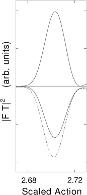
Figure 5: The peak labelled $a+3$, due to inelastic core-scattering in Fig. 2 is shown for the choice of quantum defects $\mu_{\Sigma}=0.5,$ $\mu_{\Pi}=0$. The inclusion of the higher order contributions (broken line) gives a better agreement with the quantum calculations (top) than the standard semiclassical formalism (solid line upside-down).

V Discussion and Conclusion

The feature developed in this paper is one of the many refinements that can be undertaken to improve a semiclassical formalism such as closed orbit theory. Some processes are forbidden on purely classical grounds (e.g., the above-barrier reflection of excited lithium in an electric field which results in very broad resonances in the absorption spectrum delos etal01 ) whereas other processes are semiclassically distorted (e.g., diverging amplitudes at bifurcations).

Figure 6: Recurrence spectrum for the hydrogen atom at $\epsilon=-0.55,$ $M=1,$ in the range $\gamma^{-1/3}=[30,240]$. The plot focuses on the first and second repetitions of the first-order suppressed “parallel” orbit, which is clearly visible on the quantum calculations (top). This feature is absent from the standard semiclassical calculations (bottom, solid line), but the inclusion of the higher order contributions (bottom, broken line) results in an excellent agreement with the quantum calculations. Note that the peak at $\tilde{S}=0.95$ sits on the right shoulder of the much stronger $R_{1}$ orbit; the oscillations are due to the finite range of the Welch-windowed Fourier transform.

The rôle of the perpendicular on-node orbit was first observed in calculations for the diamagnetic hydrogen atom at low scaled energy ($\epsilon\simeq-0.7$) shaw etal95 . Subsequent high-resolution experiments on helium in a magnetic field in the same dynamical regime did not clearly detect the on-node orbits (they were within the experimental noise) karremans etal99 . We have given a simpler derivation of the contribution of these first-order suppressed orbits, and our numerical results indicate that on-node orbits are more likely to be detected in non-hydrogenic atomic or molecular systems with strong quantum defects. At low scaled energies, peaks resulting from the core-scattering of the on-node orbit with a strong allowed orbit could be more easily detected; at higher scaled energies, the on-node orbit is most likely to affect the amplitude of peaks due to typical allowed orbits.

The presence of contributions in the quantum photoabsorption spectra which were not correlated with any classical orbit was observed in calculations for non-hydrogenic atoms with $m\neq 0$ in an electric field by Robicheaux and Shaw robicheaux shaw98 ; these contributions were coined “recurrences without closed orbits” because they appear at the scaled action of the parallel orbit which only exists classically when $L_{z}=0$ and should therefore be absent in an $m\neq 0$ recurrence spectrum. These authors also gave an ad-hoc semiclassical formula akin to the on-node correction which resulted in a poor agreement with the quantum calculations. Main main99 later pointed out that, for small but nonvanishing $L_{z}$, periodic orbits having nearly the same action as the $L_{z}=0$ parallel orbit do exist; it was unclear however whether the “recurrences without closed orbits” could be attributed to such orbits, in particular because the starting point of these orbits is several atomic units away from the core. Our formula Eq. (17) correctly accounts for the peaks in the recurrence spectrum associated with these apparently non-existing orbits; the $\hbar$ dependence is different to that of the suppressed on-node orbits. The physical picture is similar in both cases: just as Eq. (12) accounts for close neighbors to the on-node orbit, which are not closed at the origin but carry a portion of the wavefunction back to the core region, Eq. (17) takes into account non-radial orbits close to the $z$ axis which also give rise to recurrences by carrying the wavefunction from and into the core region.

To conclude, we have seen that first-order forbidden processes can be included within Closed-orbit theory in a simple and unified manner by elementary manipulations of the stationary phase integral, which yield a higher-order $\hbar$ dependence. In passing, we have shown that the zero degree orbit, which has always required special treatment, is in fact a case calling for a refined stationary phase integration. Analogous manipulations of the stationary phase integral of the Green’s function were performed in granger greene00 to obtain an improved semiclassical long-range scattering matrix for Rydberg atoms in fields. Our method provides a convenient and effective way of including non-radial and non-closed trajectories that nevertheless contribute to the photoabsorption spectra of Rydberg atoms and molecules in fields without the need to to calculate explicitly the involved classical dynamics of those trajectories. The validity of the method was assessed by comparing our semiclassical results to quantum calculations for Rydberg atoms and molecules in an external magnetic field.

Appendix A

We briefly work out the integral needed to determine the contribution of an orbit lying on the node of a wavefunction in Sec. III,

$$\int_{0}^{\pi}d\bar{\theta}_{f}(\bar{\theta}_{f}-\theta_{fk})^{2}\exp(i\sqrt{r_{f}/8}(\bar{\theta}_{f}-\theta_{fk})^{2}/\hbar).$$ (18)

This integral can be integrated directly but, for present purposes, it is convenient to express it in terms of sine and cosine Fresnel integrals and take the limit for the range in which the standard stationary phase approximation holds for the usual orbits. For example, in the neighborhood of $\theta_{fk}$, the real part of (18) can be expressed in the form

$$I(n) =2\int_{\theta_{fk}}^{\theta_{fk}+\varepsilon_{n}}d\bar{\theta}_{f}(\bar{\theta}_{f}-\theta_{fk})^{2}\cos(\sqrt{r_{f}/8}(\bar{\theta}_{f}-\theta_{fk})^{2}/\hbar)$$ (19)

$$=\left[-2^{3/4}\hbar^{3/2}r^{-3/4}\pi^{1/2}\right]\left\{2\mathcal{S}(\sqrt{1+2n})-2\sqrt{1+2n}\cos\pi n\right\},$$ (20)

where $\mathcal{S}$ is the sine Fresnel integral and $\varepsilon_{n}=2^{1/4}r^{-1/4}\pi^{1/2}\hbar^{1/2}\sqrt{1+2n}$ with $n$ a real number $n>-1/2$. For large half integer values of $n,$ $I(n+1)-I(n)\approx 0$ and $\mathcal{S}(\sqrt{1+2n})\sim 1/2$. $I(n)$ can then be approximated by the term between square brackets in Eq. (20). This is consistent with having neglected terms of order $(\bar{\theta}_{f}-\theta_{fk})^{4}$ in Eq. (18) provided $\hbar\rightarrow 0.$ The imaginary part of Eq. (18) is treated in the same way by writing the result in terms of the cosine Fresnel integral $\mathcal{C}(x)$. Hence

$$\int_{0}^{\pi}d\bar{\theta}_{f}(\bar{\theta}_{f}-\theta_{fk})^{2}\exp(i\sqrt{r_{f}/8}(\bar{\theta}_{f}-\theta_{fk})^{2}/\hbar)\approx\frac{\hbar^{3/2}\pi^{1/2}e^{3i\pi/4}}{r^{3/4}2^{-5/4}}.$$ (21)

Note that this result is independent of the value of $\theta_{fk}$, provided $\theta_{fk}\neq 0$.

Appendix B

A closed form expression for the integrals

$$I_{1}(\varepsilon)=\int_{0}^{\varepsilon}d\bar{\theta}_{f}\sin\bar{\theta}_{f}\exp(is\bar{\theta}_{f}^{2})$$ (22)

and

$$I_{2}(\varepsilon)=\int_{0}^{\varepsilon}d\bar{\theta}_{f}\sin\bar{\theta}_{f}\bar{\theta}_{f}^{2}\exp(is\bar{\theta}_{f}^{2}),$$ (23)

with $s$ real, are obtained in the limit in which the standard stationary phase approximation holds for the usual orbits by replacing the upper bound by $\varepsilon\rightarrow\infty$. Then Eqs. (22) and (23) are given in terms of infinite series integral table1 , which are actually representations of special functions. Choosing for simplicity a representation in terms of Fresnel integrals, Eq. (22) becomes in this limit

$$I_{1}(\infty)=\left(\frac{\pi}{2s}\right)^{1/2}\exp i\left(-\frac{1}{4s}+\frac{\pi}{2}\right)\left\{\mathcal{C}\left[(2\pi s)^{-1/2}\right]+i\mathcal{S}\left[(2\pi s)^{-1/2}\right]\right\},$$ (24)

whereas for Eq. (23) we have

$$I_{2}(\infty)=-\frac{1}{4s^{2}}\left\{1+\left(\frac{\pi}{2s}\right)^{1/2}\left(2s-i\right)\exp\left(-\frac{i}{4s}\right)\left[\mathcal{C}\left[(2\pi s)^{-1/2}\right]+i\mathcal{S}\left[(2\pi s)^{-1/2}\right]\right]\right\}.$$ (25)

When $s\rightarrow\infty,$ to first order only $\mathcal{C}\left[(2\pi s)^{-1/2}\right]\sim(2\pi s)^{-1/2}$ contributes to $I_{1}(\infty)$ whereas for $I_{2}(\infty)$ the term between the braces simply gives 2.

References

- (1) M. L. Du and J. B. Delos, Phys. Rev. A 38, 1913 (1988).
- (2) P. A. Dando, T. S. Monteiro, D. Delande, and K. T. Taylor, Phys. Rev. A 54, 127 (1996).
- (3) A. Matzkin and T. S. Monteiro, Phys. Rev. Lett. 87, 143002 (2001).
- (4) A. Matzkin, P. A. Dando, and T. S. Monteiro, Phys. Rev. A 66, 0134XX (2002).
- (5) D. A. Sadovskii and J. B. Delos, Phys. Rev. E 54, 2033 (1996).
- (6) J. Main and G. Wunner, Phys. Rev. A 55, 1743 (1997).
- (7) J. A. Shaw, J. B. Delos, M. Courtney, and D. Kleppner, Phys. Rev. A 52, 3695 (1995).
- (8) F. Robicheaux and J. Shaw, Phys. Rev. A 58, 1043 (1998)
- (9) J. Gao and J. B. Delos, Phys. Rev. A 46, 1455 (1992).
- (10) H. Friedrich and D. Wintgen, Phys. Rep. 183 , 37 (1989).
- (11) B. Hüpper, J. Main and G. Wunner, Phys. Rev. A 53, 744 (1996).
- (12) W. Schweizer, R. Niemeier, G. Wunner and H. Ruder, Z. Phys. D 25, 95 (1993).
- (13) J. B. Delos, V. Kondratovich, D. M. Wang, D. Kleppner, and N. Spellmeyer, Phys. Scripta T 90 (2001).
- (14) K. Karremans, W. Vassen, and W. Hogervorst, Phys. Rev. A 60, 2275 (1999).
- (15) J. Main, Phys. Rev. A 60, 1726 (1999).
- (16) B. E. Granger and C. H. Greene, Phys. Rev. A 62, 012511 (2000).
- (17) I. S. Gradshteyn and I. M. Ryzhik, Table of Integrals, series and products (Academic Press, Boston, 1994), Secs. 3.8-3.9.