Recognition of an organism from fragments of its complete genome

Abstract

Abstract– This paper considers the problem of matching fragment to organism using its complete genome. Our method is based on the probability measure representation of a genome. We first demonstrate that these probability measures can be modelled as recurrent iterated function systems (RIFS) consisting of four contractive similarities. Our hypothesis is that the multifractal characteristic of the probability measure of a complete genome, as captured by the RIFS, is preserved in its reasonably long fragments. We compute the RIFS of fragments of various lengths and random starting points, and compare with that of the original sequence for recognition using the Euclidean distance. A demonstration on five randomly selected organisms supports the above hypothesis.

PACS number(s): 87.14.Gg, 87.10+e, 47.53+n
Key words and phrases: complete genome, multifractal analysis, iterated function system

I Introduction

The DNA sequences of complete genomes provide essential information for understanding gene functions and evolution. A large number of these DNA sequences is currently available in public databases such as Genbank at ftp://ncbi.nlm.nih.gov/genbank/genomes/ or KEGG at http://www.genome.ad.jp/kegg/java/org_list.html). A great challenge of DNA analysis is to determine the intrinsic patterns contained in these sequences which are formed by four basic nucleotides, namely, adenine ($a$), cytosine ($c$), guanine ($g$) and thymine ($t$).

Some significant contribution results have been obtained for the long-range correlation in DNA sequences [1-16]. Li et al. [1] found that the spectral density of a DNA sequence containing mostly introns shows $1/f^{\beta}$ behaviour, which indicates the presence of long-range correlation when $0<\beta<1$. The correlation properties of coding and noncoding DNA sequences were first studied by Peng et al. [2] in their fractal landscape or DNA walk model. The DNA walk [2] was defined as that the walker steps “up” if a pyrimidine ($c$ or $t$) occurs at position $i$ along the DNA chain, while the walker steps “down” if a purine ($a$ or $g$) occurs at position $i$. Peng et al. [2] discovered that there exists long-range correlation in noncoding DNA sequences while the coding sequences correspond to a regular random walk. By undertaking a more detailed analysis, Chatzidimitriou et al. [5] concluded that both coding and noncoding sequences exhibit long-range correlation. A subsequent work by Prabhu and Claverie [6] also substantially corroborates these results. If one considers more details by distinguishing $c$ from $t$ in pyrimidine, and $a$ from $g$ in purine (such as two or three-dimensional DNA walk models [15] and maps given by Yu and Chen [16]), then the presence of base correlation has been found even in coding sequences. On the other hand, Buldyrev et al. [12] showed that long-range correlation appears mainly in noncoding DNA using all the DNA sequences available. Based on equal-symbol correlation, Voss [8] showed a power law behaviour for the sequences studied regardless of the proportion of intron contents. These studies add to the controversy about the possible presence of correlation in the entire DNA or only in the noncoding DNA. From a different angle, fractal analysis has proven useful in revealing complex patterns in natural objects. Berthelsen et al. [17] considered the global fractal dimensions of human DNA sequences treated as pseudorandom walks.

In the above studies, the authors only considered short or long DNA segments. Since the first complete genome of the free-living bacterium Mycoplasma genitalium was sequenced in 1995 [18], an ever-growing number of complete genomes has been deposited in public databases. The availability of complete genomes induces the possibility to establish some global properties of these sequences. Vieira [19] carried out a low-frequency analysis of the complete DNA of 13 microbial genomes and showed that their fractal behaviour does not always prevail through the entire chain and the autocorrelation functions have a rich variety of behaviours including the presence of anti-persistence. Yu and Wang[20] proposed a time series model of coding sequences in complete genomes. For fuller details on the number, size and ordering of genes along the chromosome, one can refer to Part 5 of Lewin [21]. One may ignore the composition of the four kinds of bases in coding and noncoding segments and only consider the global structure of the complete genomes or long DNA sequences. Provata and Almirantis [22] proposed a fractal Cantor pattern of DNA. They mapped coding segments to filled regions and noncoding segments to empty regions of a random Cantor set and then calculated the fractal dimension of this set. They found that the coding/noncoding partition in DNA sequences of lower organisms is homogeneous-like, while in the higher eucariotes the partition is fractal. This result doesn’t seem refined enough to distinguish bacteria because the fractal dimensions of bacteria computed [22] are all the same. The classification and evolution relationship of bacteria is one of the most important problems in DNA research. Yu and Anh [23] proposed a time series model based on the global structure of the complete genome and considered three kinds of length sequences. After calculating the correlation dimensions and Hurst exponents, it was found that one can get more information from this model than that of fractal Cantor pattern. Some results on the classification and evolution relationship of bacteria were found [23]. The correlation property of these length sequences has been discussed [24]. The multifractal analysis for these length sequences was done in [25].

Although statistical analysis performed directly on DNA sequences has yielded some success, there has been some indication that this method is not powerful enough to amplify the difference between a DNA sequence and a random sequence as well as to distinguish DNA sequences themselves in more details [26]. One needs more powerful global and visual methods. For this purpose, Hao et al. [26] proposed a visualisation method based on counting and coarse-graining the frequency of appearance of substrings with a given length. They called it the portrait of an organism. They found that there exist some fractal patterns in the portraits which are induced by avoiding and under-represented strings. The fractal dimension of the limit set of portraits was also discussed [27, 28]. There are other graphical methods of sequence patterns, such as chaos game representation [29, 30].

Yu et al. [31] introduced a representation of a DNA sequence by a probability measure of $k$-strings derived from the sequence. This probability measure is in fact the histogram of the events formed by all the $k$-strings in a dictionary ordering. It was found [31] that these probability measures display a distinct multifractal behaviour characterised by their generalised Rényi dimensions (instead of a single fractal dimension as in the case of self-similar processes). Furthermore, the corresponding $C_{q}$ curves (defined in [32]) of these generalised dimensions of all bacteria resemble classical phase transition at a critical point, while the “analogous” phase transitions (defined in [32]) of chromosomes of nonbacteria exhibit the shape of double-peaked specific heat function. These patterns led to a meaningful grouping of archaebacteria, eubacteria and eukaryote. Anh et al. [33] took a further step in providing a theory to characterise the multifractality of the probability measures of the complete genomes. In particular, the resulting parametric models fit extremely well the $D_{q}$ curves of the generalised dimensions and the corresponding $K_{q}$ curves of the above probability measures of the complete genomes.

A conclusion of the work reported in Yu et al. [31] and Anh et al. [33] is that the histogram of the $k$-strings of the complete genome provides a good representation of the genome and that these probability measures are multifractal. This multifractality is, in most cases studied, characteristic of the DNA sequences, hence can be used for their classification.

In this paper, we consider the problem of recognition of an organism based on fragments of their DNA sequences. The identification of the organisms in a culture commonly relies on their molecular identity markers such as the genes that code for ribosomal RNA. However, it is usual that most fragments lack the marker, “making the task of matching fragment to organism akin to reconstructing a document that has been shredded” (M. Leslie, “Tales of the sea”, New Scientist, 27 January 2001). A well-known method to tackle the task is the random shotgun sequencing method, which scans the sequences of all fragments looking for overlaps to be able to piece the fragments together. It is obvious that this technique is extremely time-consuming and many crucial fragments may be missing.

This paper will provide a different method to approach this problem. Our starting point is the probability measure of the $k$-strings and its multifractality. We model this multifractality using a recurrent iterated function system ([34, 35]) consisting of four contractive similarities (to be described in Section IV). This branching number of four is a natural consequence of the four basic elements ($a,c,g,t)$ of the DNA sequences. Each of these RIFS is specified by a matrix of incidence probabilities ${\bf P}=(p_{ij}),$ $i,j=1,...,4,$ with $p_{i1}+p_{i2}+p_{i3}+p_{i4}=1$ for $i=1,...,$ $4.$ It is our hypothesis that, for reasonably-long fragments, the multifractal characteristic of the measure of a complete genome as captured by the matrix $\mathbf{P}$ is preserved in the fragments. We thus represent each fragment by a vector $({\frac{1}{4}}\left(p_{11}+p_{21}+p_{31}+p_{41}\right)$ , ${\frac{1}{4}}\left(p_{12}+p_{22}+p_{32}+p_{42}\right)$ , ${\frac{1}{4}}\left(\,p_{13}+p_{23}+p_{33}+p_{43}\right)$ in ${\bf R}_{+}^{3}.$ We will see that, for fragments of lengths longer than 1/20 of the original sequence and with random starting points, these vectors are very close, using the Euclidean distance, to the vector of the complete sequence.

We will demonstrate the technique on five organisms, namely, A. fulgidus, B. burgdorferi, C. trachomatis, E. coli and M. genitalium. As remarked in Yu et al. [31], substrings of length $k=6$ are sufficient to represent DNA sequences. For each organism, we compute the histograms for the 6-strings of its complete genome, and 4 cases of fragments of lengths 1/4, 1/8, 1/15 and 1/20 of the complete sequence. The starting position of each fragment is chosen randomly. The RIFS of the complete genome and each of the fragments are computed next. The numerical results are reported in Section V. Some conclusions will be drawn in Section VI.

II Measure representation of complete genomes

We first outline the method of Yu et al. [31] in deriving the measure representation of a DNA sequence. We call any string made up of $k$ letters from the set $\{g,c,a,t\}$ a $k$-string. For a given $k$ there are in total $4^{k}$ different $k$-strings. In order to count the number of each kind of $k$-strings in a given DNA sequence, $4^{k}$ counters are needed. We divide the interval $[0,1)$ into $4^{k}$ disjoint subintervals, and use each subinterval to represent a counter. Letting $s=s_{1}\cdots s_{k},\,s_{i}\in\{a,c,g,t\},i=1,\cdots,k,$ be a substring with length $k$, we define

$$x_{l}(s)=\sum_{i=1}^{k}\frac{x_{i}}{4^{i}},$$ (1)

where

$$x_{i}=\left\{\begin{array}[]{l}0,\ \ \ \mbox{if}\ s_{i}=a,\\ 1,\ \ \ \mbox{if}\ s_{i}=c,\\ 2,\ \ \ \mbox{if}\ s_{i}=g,\\ 3,\ \ \ \mbox{if}\ s_{i}=t,\end{array}\right.$$ (2)

and

$$x_{r}(s)=x_{l}(s)+\frac{1}{4^{k}}.$$ (3)

We then use the subinterval $[x_{l}(s),x_{r}(s))$ to represent substring $s$. Let $N(s)$ be the times of substring $s$ appearing in the complete genome. If the number of bases in the complete genome is $L$, we define

$$F(s)=N(s)/(L-k+1)$$ (4)

to be the frequency of substring $s$. It follows that $\sum_{\{s\}}F(s)=1$. We can now view $F(s)$ as a function of $x$ and define a measure $\mu_{k}$ on $[0,1)$ by

$$\mu_{k}\left(x\right)=Y_{k}\left(x\right)dx,$$

where

$$Y_{k}(x)=4^{k}F_{k}(s),\ \ \ \ x\in[x_{l}(s),x_{r}(s)).$$ (5)

We then have $\mu_{k}\left([0,1)\right)=1$ and $\mu_{k}\left([x_{l}(s),x_{r}(s))\right)=F_{k}(s).$ We call $\mu_{k}\left(x\right)$ the  measure representation of an organism. As an example, the measure representation of M. genitalium for $k=3,...,6$ is given in FIG. 1. A fractal-like behaviour is apparent in the measures.

Remark: The ordering of $a,c,g,t$ in (2) follows the natural dictionary ordering of $k$-strings in the one-dimensional space. A different ordering of $a,c,g,t$ would change the nature of the correlations of the measure. But in our case, a different ordering of $a,c,g,t$ in Eq. (2) gives the same multifractal spectrum ($D_{q}$ curve which will be defined in the next section) when the absolute value of $q$ is relatively small (see FIG. 2 in [31]). Hence the multifractal characteristic is independent of the ordering. In the comparison of different organisms using the measure representation, once the ordering of $a,c,g,t$ in (2) is given, it is fixed for all organisms [31].

III Multifractal analysis

The most common algorithms of multifractal analysis are the so-called fixed-size box-counting algorithms [36]. In the one-dimensional case, for a given measure $\mu$ with support $E\subset{\bf R}$, we consider the partition sum

$$Z_{\epsilon}(q)=\sum_{\mu(B)\neq 0}[\mu(B)]^{q},$$ (6)

$q\in{\bf R}$, where the sum runs over all different nonempty boxes $B$ of a given side $\epsilon$ in a grid covering of the support $E$, that is,

$$B=[k\epsilon,(k+1)\epsilon[.$$ (7)

The exponent $\tau(q)$ is defined by

$$\tau(q)=\lim_{\epsilon\rightarrow 0}\frac{\log Z_{\epsilon}(q)}{\log\epsilon}$$ (8)

and the generalized fractal dimensions of the measure are defined as

$$D_{q}=\tau(q)/(q-1),\ \ \mbox{for}\ q\neq 1,$$ (9)

and

$$D_{q}=\lim_{\epsilon\rightarrow 0}\frac{Z_{1,\epsilon}}{\log\epsilon},\ \ \mbox{for}\ q=1,$$ (10)

where $Z_{1,\epsilon}=\sum_{\mu(B)\neq 0}\mu(B)\log\mu(B)$. The generalized fractal dimensions are estimated through a linear regression of

$\displaystyle\frac{1}{q-1}\log Z_{\epsilon}(q)$

against $\log\epsilon$ for $q\neq 1$, and similarly through a linear regression of $Z_{1,\epsilon}$ against $\log\epsilon$ for $q=1$. $D_{1}$ is called information dimension and $D_{2}$ is called correlation dimension. The $D_{q}$ of the positive values of $q$ give relevance to the regions where the measure is large, i.e., to the $k$-strings with high probability. The $D_{q}$ of the negative values of $q$ deal with the structure and the properties of the most rarefied regions of the measure.

IV IFS and RIFS models and the moment method for parameter estimation

In this paper, we propose to model the measure defined in Section II for a complete genome by a recurrent IFS. As we work with measures on compact intervals, the theory of Section II is narrowed down to the one-dimensional case (i.e. $d=1).$ Consider a system of contractive maps $S=\{S_{1},S_{2},\cdots,S_{N}\}$. Let $E_{0}$ be a compact interval of ${\bf R}$, $E_{\sigma_{1}\sigma_{2}\cdots\sigma_{n}}=S_{\sigma_{1}}\circ S_{\sigma_{2}}\circ\cdots\circ S_{\sigma_{n}}(E_{0})$ and

$$E_{n}=\cup_{\sigma_{1},\cdots,\sigma_{n}\in\{1,2,\cdots,N\}}E_{\sigma_{1}\sigma_{2}\cdots\sigma_{n}}.$$

Then $E=\cap_{n=1}^{\infty}E_{n}$ is the attractor of the IFS. Given a set of probabilities $p_{i}>0,\ \sum_{i=1}^{N}p_{i}=1$, we pick an $x_{0}\in E$ and define iteratively the sequence

$$x_{n+1}=S_{\sigma_{n}}(x_{n}),\qquad\quad n=0,1,2,\cdots,$$ (11)

where the indices $\sigma_{n}$ are chosen randomly and independently from the set $\{1,2,\cdots,N\}$ with probabilities $P(\sigma_{n}=i)=p_{i}$. Then every orbit $\{x_{n}\}$ is dense in the attractor $E$ [37, 38]. For $n$ large enough, we can view the orbit $\{x_{0},x_{1},\cdots,x_{n}\}$ as an approximation of $E$. This iterative process is called a chaos game.

Given a system of contractive maps $S=\{S_{1},S_{2},\cdots,S_{N}\}$ on a compact metric space $E^{\ast}$, we associate with these maps a matrix of probabilities ${\bf P}=(p_{ij})$ such that $\sum_{j}p_{ij}=1,\ i=1,2,\cdots,N$. Consider a random sequence generated by a chaos game:

$$x_{n+1}=S_{\sigma_{n}}(x_{n}),\quad n=0,1,2,\cdots,$$ (12)

where $x_{0}$ is any starting point and $\sigma_{n}$ is chosen with a probability that depends on the previous index $\sigma_{n-1}$:

$$P(\sigma_{n+1}=i)=p_{\sigma_{n},i}.$$ (13)

The choice of the indices $\sigma_{n}$ as prescribed by (13) presents a fundamental difference between this iterative process and that defined by (11) of the usual chaos game. Then $(E^{\ast},S,{\bf P})$ is called a recurrent IFS. The flexibility of RIFS permits the construction of more general sets and measures which do not have to exhibit the strict self-similarity of IFS. This would offer a more suitable framework to model fractal-like objects and measures in nature.

Let $\mu$ be the invariant measure on the attractor $E$ of an IFS or RIFS, $\chi_{B}$ the characteristic function for the Borel subset $B\subset E$; then from the ergodic theorem for IFS or RIFS [37],

$$\mu(B)=\lim_{n\rightarrow\infty}[\frac{1}{n+1}\sum_{k=0}^{n}\chi_{b}(x_{k})].$$ (14)

In other words, $\mu(B)$ is the relative visitation frequency of $B$ during the chaos game. A histogram approximation of the invariant measure may then be obtained by counting the number of visits made to each pixel on the computer screen.

The coefficients in the contractive maps and the probabilities in the IFS or RIFS model are the parameters to be estimated for a given measure which we want to simulate. Vrscay [38] introduced a moment method to perform this task. If $\mu$ is the invariant measure and $E$ the attractor of the IFS or RIFS in ${\bf R}$, the moments of $\mu$ are

$$g_{i}=\int_{E}x^{i}d\mu,\qquad g_{0}=\int_{E}d\mu=1.$$ (15)

If $S_{i}(x)=c_{i}x+d_{i},\ i=1,\cdots,N$, then the following well-known recursion relations hold for the IFS model:

$$[1-\sum_{i=1}^{N}p_{i}c_{i}^{n}]g_{n}=\sum_{j=1}^{n}\left(\begin{array}[]{l}n\\ j\end{array}\right)g_{n-j}(\sum_{i=1}^{N}p_{i}c_{i}^{n-j}d_{i}^{j}).$$ (16)

Thus, setting $g_{0}=1$, the moments $g_{n},\ n\geq 1$, may be computed recursively from a knowledge of $g_{0},\cdots,g_{n-1}$ [38].

For the RIFS model, we have

$$g_{n}=\sum_{j=1}^{N}g_{n}^{(j)},$$ (17)

where $g_{n}^{(j)},\ j=1,\cdots,N$, are given by the solution of the following system of linear equations:

$$\sum_{j=1}^{N}(p_{ji}c_{i}^{n}-\delta_{ij})g_{n}^{(j)} = -\sum_{k=0}^{n-1}\left(\begin{array}[]{l}n\\ k\end{array}\right)[\sum_{j=1}^{N}c_{i}^{k}d_{i}^{n-k}p_{ji}g_{k}^{(j)}],$$ (21)

$$i=1,\cdots,N,\ n\geq 1.$$

For $n=0$, we set $g_{0}^{(i)}=m_{i}$, where $m_{i}$ are given by the solution of the linear equations

$$\sum_{j=1}^{N}p_{ji}m_{j}=m_{i},\quad i=1,2,\cdots,N,\quad g_{0}=\sum_{i=1}^{N}m_{i}=1.$$ (22)

If we denote by $G_{k}$ the moments obtained directly from a given measure using (15), and $g_{k}$ the formal expression of moments obtained from (16) for the IFS model or from (17-22) for the RIFS model, then through solving the optimal problem

$$\min_{c_{i},d_{i},p_{i}\mbox{ or }p_{ij}}\sum_{k=1}^{n}(g_{k}-G_{k})^{2},\qquad\mbox{for some chosen}\ n,$$ (23)

we can obtain the estimates of the parameters in the IFS or RIFS model.

From the measure representation of a complete genome, it is natural to choose $N=4$ and

$$S_{1}(x)=x/4,\ S_{2}(x)=x/4+1/4,$$

$$S_{3}(x)=x/4+1/2,\ S_{4}(x)=x/4+3/4$$

in the IFS or RIFS model. Based on the estimated values of the probabilities, we can use the chaos game to generate a histogram approximation of the invariant measure of the IFS or RIFS, which then can be compared with the given measure of the complete genome.

V Application to the recognition problem

The measure representations for a large number of complete genomes, as described in Section II, were obtained in Yu et al. [31]. It was found that substrings with $k=6$ seem to provide a limiting measure that can be used for the classification and recognition of DNA sequences. Hence we will use 6-strings in this paper. We then estimated their IFS and RIFS models using the moment method described in Section 4. The chaos game algorithm was next performed to generate an orbit as in (11) or (12) with (13). From these orbits, simulated approximations of the invariant measures of IFS or RIFS were obtained via the ergodic theorem (14). In order to clarify how close the simulated measure is to the original measure, we convert a measure to its walk representation: We denote by $\{t_{j},\ j=1,2,\cdots,4^{k}\}$ the density of a measure and $t_{ave}$ its average, then define the walk $T_{j}=\sum_{k=1}^{j}(t_{k}-t_{ave}),\ j=1,2,\cdots,4^{k}$. The two walks of the given measure and the measure generated by the chaos game of an IFS or RIFS are then plotted in the same figure for comparison. We found that RIFS is a better model to simulate complete genomes. We determine the ”goodness” of the measure simulated from the RIFS model relative to the original measure based on the following relative standard error (RSE)

$$RSE=\frac{RMSE}{SE},$$

where

$$RMSE=\sqrt{\frac{1}{4^{6}}\sum_{j=1}^{4^{6}}(t_{j}-\hat{t}_{j})^{2}},$$

and

$$SE=\sqrt{\frac{1}{4^{6}}\sum_{j=1}^{4^{6}}(t_{j}-t_{ave})^{2}},$$

$(t_{j})_{j=1}^{4^{6}}$ and $(\hat{t}_{j})_{j=1}^{4^{6}}$ being the densities of the original measure and the RIFS simulated measure respectively. The goodness of fit is indicated by the result $RSE\ <\ 1$. For example, the RIFS simulation of 6-strings measure representation of M. genitalium is shown in the left figure of FIG. 2, and the walk of its original 6-strings measure representation and that simulated from the corresponding RIFS are shown in the right figure of FIG. 2. For the whole genome, $RMSE=0.00020675$, $SE=0.0003207$ and $RSD=0.6447\ <\ 1$. It is seen that the RIFS simulation fits the original measure very well.

We next pick out five organisms (without any particular a priori reason) from about 50 organisms whose complete genomes are currently available. These are A. fulgidus, B. burgdorferi, C. trachomatis, E. coli and M. genitalium. Fragments of different length rates ranging from 1/20 to 1/4 and with random starting points along the sequences were then selected. Here the length rate of a fragment means the length of this fragment divided by the length of the genome of the same organism. For example, the measure representations of different fragments of M. genitalium are shown in FIG. 3. The RIFS model for each of these fragments was next estimated. We also show the RIFS simulation of the 6-strings measure representation of the 1/20 fragment of M. genitalium in the left figure of FIG. 4. The walk of its original 6-strings measure representation and that of RIFS simulation are shown in the right figure of FIG. 4. For this fragment, $RMSE=0.00023169$, $SE=0.00035475$ and $RSD=0.6531\ <\ 1$. Again, the RIFS simulation fits the original measure of this fragment very well.

It should be noted that column $i$ in the matrix $\mathbf{P}$ describes the activity of similarity $S_{i}$ in each RIFS. To be able to represent each fragment on a three-dimensional plot, we define

$$\left\{\begin{array}[]{l}P_{1}=(p_{11}+p_{21}+p_{31}+p_{41})/4,\\ P_{2}=(p_{12}+p_{22}+p_{32}+p_{42})/4,\\ P_{3}=(p_{13}+p_{23}+p_{33}+p_{43})/4.\end{array}\right.$$ (24)

Each fragment is then represented by the vector $\left(P_{1},P_{2},P_{3}\right).$ The values of these vectors are provided in Table I, and the vectors are plotted in FIG. 5. It is seen that the vectors of the fragments from the same organism cluster together, and this clustering holds for all selected lengths. This accuracy is uniform for all five organisms randomly selected.

In matching a fragment to organism, the $D_{q}$ curve, which depicts the generalised dimension of the invariant measure as described in Section III, can also be used. We computed these curves for the above five organisms at a variety of length sizes, to 1/100th of the original sequence. The results were reported for M. genitalium in FIG. 6. It is seen that this method also performs very well. However, it suffers a drawback that many different organisms seem to have the same or closely related $D_{q}$ curve. In this sense, the method based on the RIFS has higher resolution in distinguishing the genomes. If necessary, the entire matrix $\mathbf{P}$ may be used, instead of (24), in this comparison. This would enhance the matching, but will not be as economical as (24). Yu et al. [39] used the entire matrix P to define the distance between two organisms in higher dimensional space and then the evolutionary tree of more than 50 organisms was constructed. The RIFS model can also be used to simulate the measure representation of proteins based on the HP model [40].

VI Conclusion

This paper provides a method for matching fragment to organism taking advantage of the multifractal characteristic of the measure representation of their genomes. It was demonstrated empirically that the underlying mechanism of this multifractality can be captured by a recurrent IFS, whose theory is well founded in the fractal geometry literature. Fast algorithms for the computation of these RIFS and related quantities as well as tools for comparison are available. The method seems to work reasonably well with low computing cost. This fast and economical method can be performed at a preliminary stage to cluster fragments before a more extensive method, such as the random shotgun sequencing method as mentioned in the Introduction, is decided to be brought in for higher accuracy.

TABLE I.: Values of vector representation $(P_{1},P_{2},P_{3})$ of fragments from the five organisms.

Organism	Sequence	$P_{1}$	$P_{2}$	$P_{3}$
	1/4 fragment	0.255114	0.248454	0.234208
	1/8 fragment	0.257610	0.248891	0.232988
A. fulgidus	1/15 fragment	0.260611	0.245235	0.229882
	1/20 fragment	0.253536	0.247569	0.233501
	whole genome	0.257277	0.248579	0.233379
	1/4 fragment	0.305165	0.160478	0.165485
	1/8 fragment	0.303635	0.160063	0.166952
B. burgdorferi	1/15 fragment	0.351298	0.188586	0.135497
	1/20 fragment	0.310800	0.163463	0.162279
	whole genome	0.335605	0.173103	0.143191
	1/4 fragment	0.293139	0.226877	0.197907
	1/8 fragment	0.275901	0.220717	0.206184
C. trachomatis	1/15 fragment	0.299231	0.226269	0.194245
	1/20 fragment	0.293706	0.219299	0.192447
	whole genome	0.284452	0.223418	0.201998
	1/4 fragment	0.253291	0.253147	0.237551
	1/8 fragment	0.250753	0.250494	0.240300
E. coli	1/15 fragment	0.256441	0.248731	0.232963
	1/20 fragment	0.252115	0.252027	0.237276
	whole genome	0.248986	0.255393	0.242893
	1/4 fragment	0.339263	0.165702	0.140649
	1/8 fragment	0.335415	0.187653	0.158851
M. genitalium	1/15 fragment	0.337408	0.173610	0.144801
	1/20 fragment	0.336145	0.182237	0.149540
	whole genome	0.335212	0.175269	0.147534

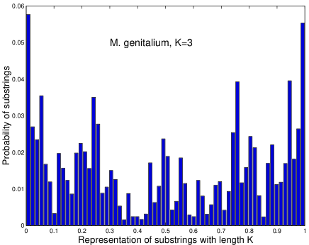
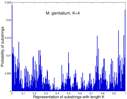
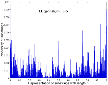
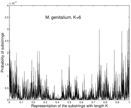
FIG. 1.: Histograms of substrings with different lengths

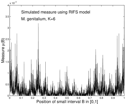
FIG. 2.: Left): Simulation of the measure representation (6-strings) of the whole genome of M. genitalium using the recurrent IFS model. Right): Walk comparison for measure representation (6-strings) of M. genitalium and its RIFS simulation.

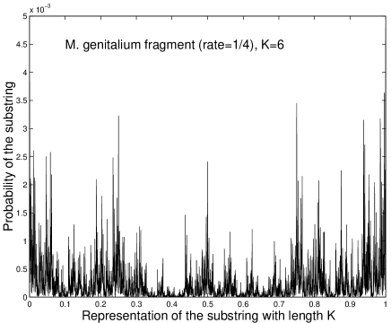
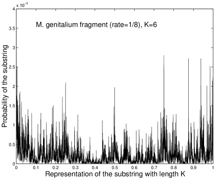
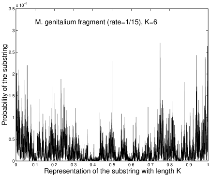
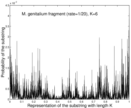
FIG. 3.: Histograms of 6-substrings of fragments from M. genitalium with different rates.

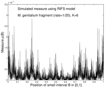
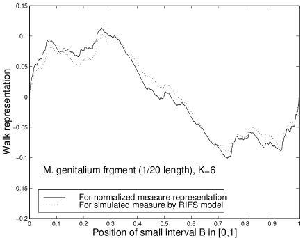
FIG. 4.: Left): Simulation of the measure representation (6-strings) of 1/20 fragment of M. genitalium using the recurrent IFS model. Right): Walk comparison for measure representation (6-strings) of 1/20 fragment of M. genitalium and its RIFS simulation.

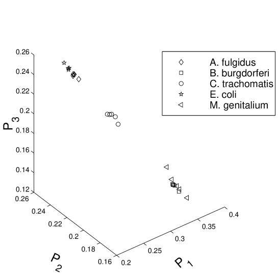
FIG. 5.: Vector representation ($P_{1},P_{2},P_{3})$) of all fragments from five organisms.

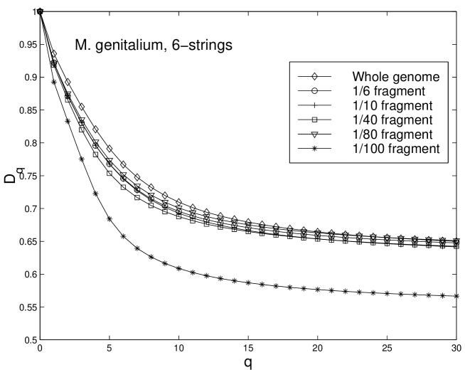
FIG. 6.: The dimension spectra of fragments from M. genitalium.

REFERENCES

- [1] W. Li and K. Kaneko, Europhys. Lett. 17, 655 (1992); W. Li, T. Marr, and K. Kaneko, Physica D 75, 392 (1994).
- [2] C.K. Peng, S. Buldyrev, A.L.Goldberg, S. Havlin, F. Sciortino, M. Simons, and H.E. Stanley, Nature 356, 168 (1992).
- [3] J. Maddox, Nature 358, 103 (1992).
- [4] S. Nee, Nature 357, 450 (1992).
- [5] C.A. Chatzidimitriou-Dreismann and D. Larhammar, Nature 361, 212 (1993).
- [6] V.V. Prabhu and J. M. Claverie, Nature 359, 782 (1992).
- [7] S. Karlin and V. Brendel, Science 259, 677 (1993).
- [8] (a) R. Voss, Phys. Rev. Lett. 68, 3805 (1992); (b) Fractals 2, 1 (1994).
- [9] H.E. Stanley, S.V. Buldyrev, A.L. Goldberg, Z.D. Goldberg, S. Havlin, R.N. Mantegna, S.M. Ossadnik, C.K. Peng, and M. Simons, Physica A 205, 214 (1994).
- [10] H.Herzel, W. Ebeling, and A.O. Schmitt, Phys. Rev. E 50, 5061 (1994).
- [11] P. Allegrini, M. Barbi, P. Grigolini, and B.J. West, Phys. Rev. E 52, 5281 (1995).
- [12] S. V. Buldyrev, A. L. Goldberger, S. Havlin, R. N. Mantegna, M. E. Matsa, C. K. Peng, M, Simons, and H. E. Stanley, Phys. Rev. E 51(5), 5084 (1995).
- [13] A. Arneodo, E. Bacry, P.V. Graves, and J. F. Muzy, Phys. Rev. Lett. 74, 3293 (1995).
- [14] A. K. Mohanty and A.V.S.S. Narayana Rao, Phys. Rev. Lett. 84(8), 1832 (2000).
- [15] L. Luo, W. Lee, L. Jia, F. Ji and L. Tsai, Phys. Rev. E 58(1), 861 (1998).
- [16] Z. G. Yu and G. Y. Chen, Comm. Theor. Phys. 33(4), 673 (2000).
- [17] C. L. Berthelsen, J. A. Glazier and M. H. Skolnick, Phys. Rev. A 45(12), 8902 (1992).
- [18] C. M. Fraser et al., The minimal gene complement of Mycoplasma genitalium, Science, 270, 397 (1995).
- [19] Maria de Sousa Vieira, Statistics of DNA sequences: A low-frequency analysis, Phys. Rev. E 60(5), 5932 (1999).
- [20] Z. G. Yu and B. Wang, Chaos, Solitons and Fractals 12(3), 519 (2001).
- [21] B. Lewin, Genes VI, Oxford University Press, 1997.
- [22] A. Provata and Y. Almirantis, Fractals 8(1), 15 (2000).
- [23] Z. G. Yu and V. V. Anh, Chaos, Soliton and Fractals 12(10), 1827 (2001).
- [24] Z. G. Yu, V. V. Anh and Bin Wang, Phys. Rev. E 63, 11903 (2001).
- [25] Z. G. Yu, V. V. Anh and K. S. Lau, Physica A 301(1-4), 351 (2001).
- [26] B. L. Hao, H. C. Lee, and S. Y. Zhang, Chaos, Solitons and Fractals, 11(6), 825 (2000).
- [27] Z. G. Yu, B. L. Hao, H. M. Xie and G. Y. Chen, Chaos, Solitons and Fractals 11(14), 2215 (2000).
- [28] B. L. Hao, H. M. Xie, Z. G. Yu and G. Y. Chen, Physica A 288, 10 (2001).
- [29] H. J. Jeffrey, Nucleic Acids Research 18(8), 2163 (1990).
- [30] N. Goldman, Nucleic Acids Research 21(10), 2487 (1993).
- [31] Z. G. Yu, V. V. Anh and K. S. Lau, Phys. Rev. E 64, 031903 (2001).
- [32] E. Canessa, J. Phys. A: Math. Gen. 33, 3637 (2000).
- [33] V. V. Anh, K. S. Lau and Z. G. Yu, J. Phys. A: Math. Gene. 34, 7127 (2001).
- [34] M.F. Barnsley, J.H. Elton and D.P. Hardin, Constr. Approx. B 5, 3 (1989).
- [35] K.S. Lau and S.M. Ngai, Adv. Math. 141, 45 (1999).
- [36] T. Halsy, M. Jensen, L. Kadanoff, I. Procaccia, and B. Schraiman, Phys. Rev. A 33, 1141 (1986).
- [37] M.F. Barnsley and S. Demko, Proc. Roy. Soc. London A 399, 243 (1985).
- [38] E. R. Vrscay, in Fractal Geometry and analysis, Eds, J. Belair, NATO ASI series, Kluwer Academic Publishers, 1991.
- [39] Z. G. Yu, V. V. Anh, K. S. Lau and K. H. Chu, Phylogenetic analysis of living organisms based on a fractal model of complete genomes. Submitted to J. Mol. Evol..
- [40] Z. G. Yu, V. V. Anh and K. S. Lau, Fractal analysis of measure representation of large proteins based on the detailed HP model. Submitted to J. Chem. Phys.