Mixed configuration-interaction and many-body perturbation theory calculations of energies and oscillator strengths of J=1 odd states of neon

Abstract

Ab-initio theory is developed for energies of $J=1$ particle-hole states of neutral neon and for oscillator strengths of transitions from such states to the $J=0$ ground state. Hole energies of low-$Z$ neonlike ions are evaluated.

I Introduction

A combined configuration-interaction (CI) many-body-perturbation-theory (MBPT) method, applied previously to divalent atoms Savukov and Johnson (2002), is extended to particle-hole states of closed-shell atoms. After derivation of CI+MBPT expressions for particle-hole states, we will apply the theory to calculations of energies and electric-dipole transition probabilities for neon.

For neon, many accurate measurements of transition rates are available, providing important tests of theory. Reciprocally, the theory might help resolve existing discrepancies among oscillator strengths ($f$-values) for transitions from the ground state to several excited states, for which experiments disagree. There is also a certain deficiency in existing ab-initio theories in neon, for which discrepancies among many measurements and theoretical calculations are unsettled. For example, the only other elaborate ab-initio calculations (Avgoustoglou and Beck (1998)) give an oscillator strength for the $\left[2p_{3/2}^{-1}3s_{1/2}\right]_{1}$ neon state larger than most experimental values by more than two standard deviations. Extensive calculations performed by Hibbert et al. (1993) for many transition rates along the neon isoelectronic sequence use a general configuration-interaction code (CIV3) Hibbert (1975). The calculations utilize parametric adjustments with measured fine structures, but do not completely agree with experiments in neon and have an accuracy similar to other semiempirical calculations of Seaton (1998). However, the two calculations disagree with each other for several transitions. We hope that our calculations may help to understand better the theoretical problems in neon and provide guidance for the analysis of experimental data.

Some possible applications of the present CI+MBPT method include the study of neonlike ions, Ne I – Si V, S VII, Ar IX, Ca XI, and Fe XVII that have astrophysical interest and have been included in the Opacity Project (Seaton (1987)). The transition data in neon and other noble gases are also used in plasma physics, and in studying discharges that find many industrial applications in lamps and gas lasers. The methods presented here might be also used for improving the accuracy of MBPT or for extending CI+MBPT to more complicated open-shell atoms.

The principal theoretical difficulty arises from the sensitivity of transition amplitudes to the interaction between closely spaced fine-structure components. Although it is possible to obtain energies which are reasonably precise on an absolute scale using coupled-cluster methods (Ilyabaev and Kaldor (1992)), accurate fine-structure splittings seem very difficult to obtain without semiempirical adjustments. This is why semiempirical approaches, which have fine-structure intervals carefully adjusted, are more successful in neon than are ab-initio calculations. However, as we will demonstrate in this paper, CI calculations corrected with MBPT are also capable of accurately predicting fine-structure splittings and, consequently, transition amplitudes. In this paper, we will demonstrate the excellent precision of CI plus second-order MBPT. Third-order corrections, for which numerical codes already exist Avgoustoglou et al. (1992), can also be included, providing even further improvement in accuracy.

In the following section, we use the effective Hamiltonian formalism and particle-hole single-double coupled equations to derive expressions for the second-order Hamiltonian matrix of the CI+MBPT method. In the final expressions, we present a quite accurate new MBPT that can predict energies of hole states and can describe appropriately the interactions in particle-hole atoms. The accuracy of hole energies obtained with the new MBPT will be illustrated for neon and low-$Z$ neon-like ions. Our CI+MBPT energies and $f$-values for many states of neon are tabulated. Their agreement with experiment and other theories are shown.

II CI+MBPT method

The accuracy of the Rayleigh-Schrödinger variant of second-order MBPT given in Safronova et al. (2001) is insufficient for purpose, so that more accurate single-double equations must be used. The formulas for the correlation operator and a system of coupled equations for the correlation coefficients are given in Avgoustoglou et al. (1995); we follow the notation of Avgoustoglou et al. (1995) in the the paragraphs below. Under certain conditions, those equations can be further simplified and rewritten in the following form:

$$\left(\varepsilon_{b}-\varepsilon_{\alpha}\right)\chi_{b}^{\alpha} = R_{b}^{\alpha}$$

$$\left(\varepsilon_{b}+\varepsilon_{c}-\varepsilon_{\alpha}-\varepsilon_{\beta}-\widetilde{g}_{bcbc}\right)\chi_{bc}^{\alpha\beta} = R_{bc}^{\alpha\beta}-\widetilde{g}_{bcbc}\chi_{bc}^{\alpha\beta}$$

$$\left(\varepsilon_{v}-\varepsilon_{r}\right)\chi_{v}^{r} = R_{v}^{r}$$

$$\left(\varepsilon_{a}-\varepsilon_{v}\right)\chi_{v}^{a} = R_{v}^{a}$$

$$\left(\varepsilon_{v}+\varepsilon_{b}-\varepsilon_{r}-\varepsilon_{s}\right)\chi_{vb}^{rs} = R_{vb}^{rs}$$

$$\left(\varepsilon_{v}+\varepsilon_{b}-\varepsilon_{a}-\varepsilon_{s}\right)\chi_{vb}^{as} = R_{vb}^{as}\text{.}$$ (1)

In the second equation of this set, the term $\widetilde{g}_{bcbc}\chi_{bc}^{\alpha\beta}$ is subtracted from both sides of this equation to make the right-hand side small. Since large random-phase approximation (RPA) corrections in the particle-hole CI+MBPT are treated by CI, the quantities $W_{va^{\prime}}^{v^{\prime}a}$ entering this set of equations on the right-hand side in Ref. Avgoustoglou et al. (1995) are small and have been neglected here. The concern might be raised for the correlation coefficients $\chi_{vb}^{as}$ and $\chi_{v}^{r}$, which generally would have small factors $\left(\varepsilon_{v}+\varepsilon_{b}-\varepsilon_{a}-\varepsilon_{s}\right)$ or $\left(\varepsilon_{v}-\varepsilon_{r}\right)$ in front. However, for the large CI model space, energies of the core-virtual orbitals $bs$ are well separated from the energies of the valence-hole orbitals $av$. The quantities $R$ in zero approximation can be set to:

$$R_{j}^{i} = \Delta_{ij}$$

$$R_{bc}^{ij}-\tilde{g}_{bcbc}\chi_{bc}^{ij} = g_{ijbc}$$

$$R_{vb}^{is} = g_{isvb}$$ (2)

to obtain the first-order effective Hamiltonian,

$$H_{v^{\prime}a^{\prime},va}^{\text{eff}}=(\varepsilon_{v}-\varepsilon_{a})\delta_{v^{\prime}v}\delta_{a^{\prime}a}+H_{v^{\prime}aa^{\prime}v}^{(1)}$$ (3)

and the correlation coefficients $\chi$. Here we define the first-order correction $H_{v^{\prime}aa^{\prime}v}^{(1)}=\Delta_{v^{\prime}v}\delta_{a^{\prime}a}+\widetilde{g}_{v^{\prime}aa^{\prime}v}$ to the effective Hamiltonian. For faster convergence of CI and for subtraction of the dominant monopole contributions in RPA diagrams, a $V^{(N-1)}$ Hartree-Fock (HF) model potential for which $\Delta_{nm}=\widetilde{g}_{nama}$, $\Delta_{na}=\Delta_{an}=\Delta_{ab}=0$ is introduced.

Further improvement of accuracy can be achieved through iterations. After one iteration we obtain the second-order contribution to the effective Hamiltonian,

$$H_{v^{\prime}aa^{\prime}v}^{(2)}=\delta R_{v}^{v^{\prime}}\delta_{a^{\prime}a}+\delta R_{a}^{a^{\prime}}\delta_{v^{\prime}v}+\delta\widetilde{R}_{va}^{av^{\prime}}\text{,}$$ (4)

where

$$\delta R_{v}^{v^{\prime}} = \sum_{s\notin CI}\frac{\Delta_{v^{\prime}s}\Delta_{sv}}{\varepsilon_{v}-\varepsilon_{s}}$$ (5)

$$-\sum_{scd}\frac{g_{cdvs}\widetilde{g}_{v^{\prime}scd}}{\varepsilon_{c}+\varepsilon_{d}-\varepsilon_{v^{\prime}}-\varepsilon_{s}-\widetilde{g}_{cdcd}}$$

$$+\sum_{stc}\frac{g_{v^{\prime}cst}\widetilde{g}_{stvc}}{\varepsilon_{v}+\varepsilon_{c}-\varepsilon_{s}-\varepsilon_{t}}\text{,}$$

$$\delta R_{a}^{a^{\prime}} = -\sum_{scd}\frac{g_{cda^{\prime}s}\widetilde{g}_{ascd}}{\varepsilon_{c}+\varepsilon_{d}-\varepsilon_{a}-\varepsilon_{s}-\widetilde{g}_{cdcd}}$$ (6)

$$+\sum_{scd}\frac{g_{cda^{\prime}s}\widetilde{g}_{ascd}}{\varepsilon_{a^{\prime}}+\varepsilon_{c}-\varepsilon_{s}-\varepsilon_{t}-\widetilde{g}_{a^{\prime}ca^{\prime}c}}\text{,}$$

$$\delta\widetilde{R}_{va}^{av^{\prime}} = \sum_{tu}\frac{g_{av^{\prime}tu}\widetilde{g}_{tuva^{\prime}}}{\varepsilon_{v}+\varepsilon_{a^{\prime}}-\varepsilon_{t}-\varepsilon_{u}}$$ (7)

$$+\sum_{cd}\frac{\widetilde{g}_{cdva^{\prime}}g_{av^{\prime}cd}}{\varepsilon_{c}+\varepsilon_{d}-\varepsilon_{a}-\varepsilon_{v^{\prime}}-\widetilde{g}_{cdcd}}$$

$$+\sum_{t\notin CI}\frac{\widetilde{g}_{av^{\prime}ta^{\prime}}\Delta_{tv}}{\varepsilon_{v}-\varepsilon_{t}}+\sum_{dt\notin CI}\frac{\widetilde{g}_{dv^{\prime}ta^{\prime}}\widetilde{g}_{atvd}}{\varepsilon_{v}+\varepsilon_{d}-\varepsilon_{a}-\varepsilon_{t}}$$

$$-\sum_{dt}\frac{\widetilde{g}_{dv^{\prime}tv}\widetilde{g}_{ata^{\prime}d}}{\varepsilon_{a^{\prime}}+\varepsilon_{d}-\varepsilon_{a}-\varepsilon_{t}-\widetilde{g}_{a^{\prime}da^{\prime}d}}$$

$$+\sum_{t\notin CI}\frac{\Delta_{v^{\prime}t}\widetilde{g}_{taa^{\prime}v}}{\varepsilon_{v}+\varepsilon_{a^{\prime}}-\varepsilon_{t}-\varepsilon_{a}}$$

$$+\sum_{dt}\frac{\widetilde{g}_{datv}\widetilde{g}_{v^{\prime}ta^{\prime}d}}{\varepsilon_{a^{\prime}}+\varepsilon_{d}-\varepsilon_{v^{\prime}}-\varepsilon_{t}-\widetilde{g}_{a^{\prime}da^{\prime}d}}$$

$$-\sum_{dt}\frac{\widetilde{g}_{data^{\prime}}\widetilde{g}_{v^{\prime}tvd}}{\varepsilon_{v}+\varepsilon_{d}-\varepsilon_{v^{\prime}}-\varepsilon_{t}-\widetilde{g}_{adad}}.$$

Note that in the last equation we have extended the single-double method. The last term entering $\delta\widetilde{R}_{va}^{av^{\prime}}$ in the single-double formalism would normally not contain $\widetilde{g}_{adad}$ in the denominator. However, if we do not modify this denominator, we find that in the third-order MBPT, large terms proportional to $\widetilde{g}_{adad}$ will appear leading to a decrease in accuracy. A physical reason for modifying the denominator of this term is that the process described by this term contains two holes in the intermediate states with large interaction energy. This interaction should be treated nonperturbatively, for example, by inclusion of $\widetilde{g}_{adad}$ into the denominator as we have done on the basis of the single-double equations in other terms. Finally, this term is almost equal to the seventh term (they are complex conjugates and their Goldstone diagrams are related by a reflection through a horizontal axis), and for convenience they are set equal in numerical calculations. The angular reduction for $\delta\widetilde{R}_{va}^{av^{\prime}}$ can be easily obtained using the second-order particle-hole formulas given in Ref. Safronova et al. (2001).

III A solution of the hole-energy problem

III.1 Breit corrections

Apart from Coulomb correlation corrections, the Breit magnetic interaction is also important in neon and the isoelectronic ions. The breakdown of various Coulomb and relativistic contributions to the energy of $3s$ states of neon are given in Ref. Avgoustoglou et al. (1995). Breit corrections cancel, but for higher excited states they may not. Hence, to improve the accuracy of fine-structure splittings, we include the Hartree-Fock hole Breit correction $B_{aa}^{\text{(HF)}}$ in our calculations,

$$B_{aa}^{\text{(HF)}}=\sum_{c}\widetilde{b}_{acca}\text{.}$$ (8)

We have checked that the first-order corrections $B^{(1)}$ to the energies of $J=2$ and $J=1$ states given in Table I of Ref. Avgoustoglou et al. (1995) agree with our $B_{aa}^{\text{(HF)}}$ contributions, 0.00062 and 0.00090 a.u., for $2p_{3/2}$ and $2p_{1/2}$ states, respectively. We omit the small frequency-dependent Breit, quantum-electrodynamic, reduced-mass, and mass-polarization corrections. Small as they are, those corrections are further reduced after subtraction for the fine-structure intervals. More careful treatment of relativistic corrections is needed in calculations of high-$Z$ neon-like ions.

III.2 Calculations of hole energies for neonlike ions

Since we propose a new variant of the MBPT expansion, we would like first to demonstrate that this expansion is convergent for hole states. The theoretical hole energies shown in Table 1 have been obtained in the $V^{(N)}$ HF potential using Eq. (6) for $\delta R_{a}^{a}$ to calculate second-order corrections. The extra term in the denominator is important and is necessary for convergence of the perturbation expansion. Experimental hole energies in the National Institute of Standards and Technology (NIST) database Ref. nis are found as the limit energies for the neon isoelectronic sequence. For neutral neon only one limit, the p_3/2 energy is given in NIST nis . The 2p_1/2-2p_3/2 splitting 780.4269(36) cm^-1 has been measured in Ref. Harth et al. (1985), and using this value we find the experimental p_1/2 energy. Table 1 demonstrates the good agreement of our theoretical p_3/2, p_1/2 energies as well as the same fine structure interval for neon-like ions. Our fine structure interval, whose correctness is crucial for transition amplitude calculations, differs from experiment just by about 10 cm^-1. Note that the HF value 187175 cm^-1 for the 2p_3/2 state is 8.5% higher than the experimental value 173930 cm^-1, and, after adding correlation corrections, we obtain improvement by a factor of ten. For the fine structure, the HF value 1001cm^-1 disagrees even more, by 28%. If we use Rayleigh-Schrödinger perturbation theory, the corrections are twice as large as our results, and the agreement with experiment does not improve.

Table 1: A comparison of theoretical and experimental hole energies and the 2p_3/2-2p_1/2 fine-structure intervals for neon and neon-like ions. All energies are in cm^-1

	Ne	Na+	Mg+2	Al+3	Si+4
2p3/2 Th.	172434	380443	645951	967531	1344344
2p3/2 Exp.	173930	381390	646402	967804	1345070
Difference	1496	947	451	273	726
2p1/2 Th.	173218	381816	648196	970997	1349449
2p1/2 Exp.	174 710	382756	648631	971246	1350160
Difference	1492	940	435	249	711
2p3/2-2p1/2, Th.	784	1373	2245	3466	5090
2p3/2-2p1/2, Exp.	780	1366	2229	3442	5105
Difference	-4	-7	-16	-24	-15

IV Neon energies and oscillator strengths of J=1 odd states

To test the accuracy of the CI+MBPT method, we first calculated energies of several lowest odd J=1 neon states, Table 2. The number of configurations in CI was chosen to be 52. The order of eigenstates obtained in CI+MBPT is the same as the order of the experimental levels. We abbreviate long NIST designations since the levels are uniquely specified by energy or by order.

Table 2: A comparison with experiment of CI+MBPT energies referenced to the ground state and given in atomic units. An almost constant shift is subtracted in the fifth column to demonstrate excellent agreement for relative positions of levels

Level	Experiment	CI+MBPT	$\Delta$	$\Delta$ - 0.0069
$p_{3/2}^{-1}3s$	0.6126	0.6048	0.0078	0.0009
$p_{1/2}^{-1}3s$	0.6192	0.6116	0.0076	0.0007
$p_{3/2}^{-1}4s$	0.7235	0.7166	0.0070	0.0001
$p_{1/2}^{-1}4s$	0.7269	0.7200	0.0069	0.0000
$p_{3/2}^{-1}3d$	0.7360	0.7289	0.0070	0.0001
$p_{3/2}^{-1}3d$	0.7365	0.7294	0.0071	0.0002
$p_{1/2}^{-1}3d$	0.7401	0.7330	0.0071	0.0002
$p_{3/2}^{-1}5s$	0.7560	0.7491	0.0069	0.0000
$p_{1/2}^{-1}5s$	0.7593	0.7525	0.0069	0.0000

The pure ab-initio energies differ from experimental energies by 0.0069 a.u., but after subtraction of the systematic shift (which does not make much difference in transition calculations), the agreement is at the level of 0.0001 a.u. for almost all states. Therefore, we consider the accuracy of CI+MBPT adequate for correct prediction of level mixing and oscillator strengths. For the 3s states, agreement with experiment for the fine structure interval is much better than that obtained by Avgoustoglou et al. (1995), 0.0002 versus 0.0012 a.u.; a possible explanation for this could be that single-double equations miss important corrections which we included by modifying the denominators. In Ref. Avgoustoglou et al. (1995), however, the systematic shift is small.

Finally, we present our CI+MBPT oscillator strengths in neon. After diagonalization of the second-order effective Hamiltonian, we obtain wave functions in the form of expansion coefficients in the CI space and use them to calculate oscillator strengths. Size-consistent formulas for dipole matrix elements for transitions decaying into the ground state are provided in Ref. Avgoustoglou and Beck (1998), where the absorption oscillator strength $f$ is also defined. We give in this table ab-initio values of the oscillator strengths $f$. The dominant part of the RPA corrections is included at the level of CI. Small normalization corrections are omitted.

Table 3: Our CI+MBPT oscillator strengths for the ground to excited state transitions in neon compared with average experimental values (3rd and 4th columns) and those obtained with the best semiempirical theories Seaton (1998); Aleksandrov et al. (1983a); Hibbert et al. (1993)

Levels	CI+MBPT	$\sigma$-avr	mean	Ref. Seaton (1998)	Ref. Aleksandrov et al. (1983a)	Ref. Hibbert et al. (1993)
$p_{3/2}^{-1}3s$	0.0102	0.0099	0.0107	0.0126	0.0106	0.0123
$p_{1/2}^{-1}3s$	0.1459	0.1549	0.1487	0.1680	0.1410	0.1607
$p_{3/2}^{-1}4s$	0.0131	0.0122	0.123	0.0152	0.0124	-
$p_{1/2}^{-1}4s$	0.0181	0.0170	0.016	0.0193	0.0160	-
$p_{3/2}^{-1}3d$	0.0066	-	-	0.0056	0.0045	0.0047
$p_{3/2}^{-1}3d$	0.0130	0.0187	0.0199	0.0167	0.0131	0.0117
$p_{1/2}^{-1}3d$	0.0069	0.0067	0.0069	0.0086	0.0064	0.0055
$p_{3/2}^{-1}5s$	0.0068	0.0064	0.0066	0.0073	0.0060	-
$p_{1/2}^{-1}5s$	0.0053	0.0043	0.0044	0.0050	0.0043	-

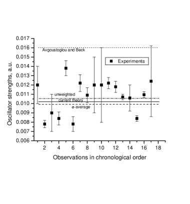
Figure 1: Comparison with experiment for oscillator strengths of the $[p_{3/2}^{-1}3s]_{1}$ state of neon

Table 4: References for experimental data shown in Fig. 1

Obs.	Reference	Year	$f$	$\sigma$
1	Kuhn et al. (1967)	1967	0.01200	0.00200
2	Lawrence and Liszt (1969)	1969	0.00780	0.00040
3	Geiger (1970)	1970	0.00900	0.00200
4	Kernahan et al. (1971)	1971	0.00840	0.00070
5	Kazantsev and Chaika (1971)	1971	0.01380	0.00080
6	Knystautas and Drouin (1974)	1974	0.00780	0.00080
7	Bhaskar and Lurio (1976)	1976	0.01220	0.00090
8	Westerveld et al. (1979)	1979	0.01090	0.00080
9	Aleksandrov et al. (1983b)	1983	0.01200	0.00300
10	Chornay et al. (1984)	1984	0.01200	0.00400
11	Tsurubuchi et al. (1989)	1990	0.01220	0.00060
12	Chan et al. (1992)	1992	0.01180	0.00060
13	Ligtenberg et al. (1994)	1994	0.01070	0.00030
14	Suzuki et al. (1994)	1994	0.01060	0.00140
15	Curtis et al. (1995)	1995	0.00840	0.00030
16	Gibson and Risley (1995)	1995	0.01095	0.00032
17	Zhong et al. (1997)	1997	0.01240	0.00380

Many experiments have disagreements in oscillator strengths far exceeding the cited errors (see Fig. 1 and Table 4): hence, for comparison, we give in Table 3 two statistical averages: the first is a weighted according to cited standard deviations and the second is an unweighted average. For the 3s levels, the experimental data compiled in Ref. Avgoustoglou and Beck (1998) and for the higher excited levels in Ref. Zhong et al. (1997) have been included in the averaging. Average values obtained here are not necessarily the most accurate, but they serve well for comparison and for a test of our probably less accurate calculated values.

A more careful analysis of experimental techniques to exclude systematic errors, which are definitely present, is necessary; our values can provide some guidance. For $p_{3/2}^{-1}3d$ states, since the energy separation of the two states is small, experiments give the sum of the two oscillator strengths, and the value 0.0196 rather than 0.0130 should be compared with the experimental values 0.0187 (0.0199). In this table, we also compare our theory with other semiempirical theories. Surprisingly, early calculations by Aleksandrov et al. (1983a) agree well with our calculations. A fair agreement, considering the high sensitivity of these transitions to correlation correction, is also obtained with the other theories in the table.

V Conclusions

In this paper, we have introduced CI+MBPT theory for particle-hole states of closed-shell atoms. A difficulty that the hole energy has poor convergence is overcome with modifications of denominators in MBPT. Good precision for hole states and for particle-hole states is illustrated for many energy levels of neon. Apart from energies, our theory is tested in calculations of oscillator strengths. Agreement with averaged experimental values is achieved.