Stochastic island generation and influence on the effective transport in stochastic magnetic fields

Abstract

The transport of collisional particles in stochastic magnetic fields is studied using the decorrelation trajectory method. The nonlinear effect of stochastic generation of magnetic island by magnetic line trapping is considered together with particle collisions. The running diffusion coefficient is determined for arbitrary values of the statistical parameters of the stochastic magnetic field and of the collisional velocity. The effect of the stochastic magnetic islands is analysed. PACS numbers: 52.35.Ra, 52.25.Fi, 05.40.-a, 02.50.-r

I
Introduction

The problem of test particle diffusion in stochastic magnetic fields was studied by many authors [1]-[13] and important progress was obtained. However, the general solution was not yet found. Particle trajectories in a magnetized plasma are determined by three stochastic processes: the magnetic field, the collisional velocity along magnetic lines and the collisional velocity perpendicular to the magnetic lines. These components of the stochastic collisional velocities have very different effects. There are two important difficulties appearing in this triple stochastic process. One is related to the parallel collisional velocity which enters as a multiplicative noise in the equations of motion and the other with the Lagrangian non-linearity which is determined by the space dependence of the stochastic magnetic field. Each of these two problems has been recently studied but only considered separately. The complete model for particle transport in stochastic magnetic fields could not be analyzed until now.

The latter difficulty can be eliminated if one restricts the study to stochastic magnetic fields with small amplitudes and/or large perpendicular correlation lengths for which the magnetic Kubo number (defined below) is small. If the perpendicular collisional velocity is neglected, this quasilinear problem has an exact solution that was obtained by several methods [14]. It shows that the parallel collisional motion determines a subdiffusive transport across the confining magnetic field with the running diffusion coefficient $D(t)$ decaying to zero as $D(t)\sim t^{-1/2}.$ It was shown [13] that this subdiffusive transport is due to collision induced trajectory trapping along the magnetic lines. The parallel collisional velocity forces the particles to return in the already visited positions along the magnetic lines and consequently generates long time Lagrangian correlation of the stochastic magnetic field. If the perpendicular collisional velocity is taken into account, the transport is diffusive and the diffusion coefficient was evaluated semi-qualitatively by several methods [1]-[11].

On the other hand, the Lagrangian non-linearity determined by the space-dependence of the stochastic magnetic field leads, at large magnetic Kubo numbers, to magnetic line trapping and generation of stochastic magnetic islands. This process is mathematically identical with the trajectory trapping in the $E\times B$ drift motion in an electrostatic turbulence. The latter was recently studied by means of a new statistical approach, the decorrelation trajectory method [15], [16].

The aim of this paper is to study the general problem of collisional particle diffusion in stochastic magnetic fields in the guiding center approximation. More specifically, we determine the effect of self-consistent generation of stochastic magnetic islands on the effective transport. The running diffusion coefficient is determined for arbitrary parameters of the stochastic magnetic field and of particle collisions. The decorrelation trajectory method is used for studying this rather complicated triple stochastic process.

The paper is organized as follows. The physical model is described in Section 2. We derive in Section 3 the Lagrangian velocity correlation and the running diffusion coefficient for arbitrary values of the four specific parameters and for given Eulerian correlation of the potential. The physical significance of this general result is then analyzed: the subdiffusive transport in Section 4, the effect of collisional cross-field diffusion in Section 5 and the effect of a time variation of the stochastic magnetic field in Section 6. The conclusions are summarized in Section 7.

II The system of equations

The particle guiding center motion is studied in a magnetic field with a stochastic component. The magnetic field is taken to be a sum of a large constant field ${\bf B}_{0}{\bf=}B_{0}{\bf e}_{z}$ and a small fluctuating field perpendicular to ${\bf B}_{0},$ and depending on the perpendicular coordinates ${\bf x}\equiv(x,y)$ and on the parallel coordinate $z$

$${\bf B}=B_{0}\left({\bf e}_{z}+{\bf b}({\bf x},z,t)\right)$$ (1)

(Here the perpendicular and the parallel directions are defined in relation to the direction of ${\bf B}_{0}).$ This is the usual slab model of the confining configuration in a tokamak plasma. Since the reduced magnetic field is divergence-free, $\nabla\cdot{\bf b}=0,$ its two components can be determined from a scalar function $\phi({\bf x},z)$ as

$${\bf b}({\bf x},z,t)={\bf\nabla}\times\phi({\bf x},z,t){\bf e}_{z}.$$ (2)

The system of equations for guiding center motion is:

$$\frac{d{\bf x}}{dt} = {\bf b}({\bf x},z,t)\eta_{\parallel}(t)+{\bf\eta}_{\perp}(t),$$ (3)

$$\frac{dz}{dt} = \eta_{\parallel}(t).$$ (4)

The three stochastic functions ${\bf b}({\bf x},z,t),$ ${\bf\eta}_{\perp}(t)$ and $\eta_{\parallel}(t)$ are statistically independent: all cross correlations are zero. All these stochastic functions are assumed to be Gaussian, stationary and homogeneous, with zero averages. The autocorrelation function of the stochastic potential $\phi({\bf x},z,t)$ is modeled by:

$$A({\bf x},z,t)\equiv\left\langle\phi({\bf 0},0,0)\,\phi({\bf x},z,t)\right\rangle=\beta^{2}\lambda_{\perp}^{2}\exp\left(-\frac{z^{2}}{2\lambda_{\perp}^{2}}-\frac{x^{2}+y^{2}}{2\lambda_{\parallel}^{2}}\right)\exp\left(-\frac{\left|t\right|}{\tau_{c}}\right)$$ (5)

where  $\beta$ is the mean square value of the reduced magnetic field ${\bf b,}$ $\lambda_{\parallel}$ is the correlation length of the potential $\phi$ along the main magnetic field ${\bf B}_{0},$ $\lambda_{\perp}$ is the correlation length in the plane perpendicular to ${\bf B}_{0}$ and $\tau_{c}$ is the correlation time of $\phi$. The autocorrelation tensor of the reduced magnetic field components $B_{ij}\equiv\left\langle b_{i}({\bf 0},0,0)b_{j}({\bf x},z,t)\right\rangle,$ $i,j=x,y,$ is determined from $A({\bf x},z)$ as

$$B_{xx}=-\frac{\partial^{2}}{\partial y^{2}}A,\quad B_{yy}=-\frac{\partial^{2}}{\partial x^{2}}A,\quad B_{xy}=\frac{\partial^{2}}{\partial x\partial y}A.$$ (6)

The collisional velocities are modeled by colored noises with the correlations

$$\left\langle\eta_{\parallel}(0)\eta_{\parallel}(t)\right\rangle_{c}=\chi_{\parallel}\nu R(\nu t)$$ (7)

$$\left\langle\eta_{\perp}^{i}(0)\eta_{\perp}^{j}(t)\right\rangle_{c}=\delta_{ij}\chi_{\perp}\nu R(\nu t)$$ (8)

where $\nu$ is the collision frequency, $\chi_{\parallel}=\lambda_{mfp}^{2}\nu/2$ is the parallel collisional diffusivity, $\lambda_{mfp}$ is the parallel mean free path, $\chi_{\perp}=\rho_{L}^{2}\nu/2$  is the perpendicular collisional diffusivity and $\rho_{L}$ is the Larmor radius relative to the reference field. $R(\nu t)$ is a time decreasing function that is chosen as

$$R(\nu t)=\exp(-\nu\left|t\right|)$$ (9)

for the explicit calculations presented in this paper.

We introduce dimensionless quantities with the following units: $\lambda_{\perp}$ for the perpendicular displacements, $\lambda_{\parallel}$ for the displacements along the reference magnetic field and $\nu^{-1}$ for the time. The perpendicular velocity ${\bf v}={\bf b}\eta_{\parallel}$ is reduced with $V\equiv\beta\sqrt{\chi_{\parallel}\nu}$, the parallel velocity $\eta_{\parallel}(t)$ with $\sqrt{\chi_{\parallel}\nu}$ and the perpendicular collisional velocity ${\bf\eta}_{\perp}(t)$ with $\sqrt{\chi_{\perp}\nu}.$ The equations of motion in these dimensionless variables (denoted by the same symbols as the physical ones) are:

$$\frac{d{\bf x}}{dt}=M\,{\bf b}({\bf x},z,t)\eta_{\parallel}(t)+\overline{\chi}_{\perp}^{1/2}{\bf\eta}_{\perp}(t)$$ (10)

$$\frac{dz}{dt}=\overline{\chi}_{\parallel}^{1/2}\eta_{\parallel}(t).$$ (11)

Four dimensionless parameters appear naturally in this problem: the dimensionless perpendicular and respectively parallel diffusivities

$$\overline{\chi}_{\perp}\equiv\frac{\chi_{\perp}}{\lambda_{\perp}^{2}\nu},\qquad\overline{\chi}_{\parallel}\equiv\frac{\chi_{\parallel}}{\lambda_{\parallel}^{2}\nu},$$ (12)

a dimensionless parameter that contains the effect of the stochastic magnetic field

$$M=\frac{V}{\lambda_{\perp}\nu}=\frac{\beta\lambda_{\parallel}}{\lambda_{\perp}}\overline{\chi}_{\parallel}^{1/2},$$ (13)

and the dimensionless decorrelation time:

$$\overline{\tau}_{c}=\tau_{c}\nu.$$ (14)

We note that the parameter which describes the evolution of the magnetic lines, the magnetic Kubo number $K_{m}=\beta\lambda_{\parallel}/\lambda_{\perp},$ appears here as a factor in $M,$ which can be written as $M=K_{m}\overline{\chi}_{\parallel}^{1/2}.$

The aim of this calculation is to determine the Lagrangian correlation of the effective perpendicular velocity

$${\bf v(x},z,t{\bf)\equiv b}({\bf x},z,t)\eta_{\parallel}(t)$$ (15)

which leads to the perpendicular effective diffusion coefficient.

III Solution by the decorrelation trajectory method

We use the decorrelation trajectory method following the recent calculations for the influence of particle collisions on the diffusion in electrostatic turbulence [16]. The difference and the supplementary difficulty of the magnetic problem comes from the structure (15) of the velocity ${\bf v}$ which is the product of two stochastic processes. They are statistically independent but in the Lagrangian frame they are correlated through the trajectories due to the space dependence of the magnetic field fluctuations. The later makes this problem strongly nonlinear. The trajectories also depend on the collisional velocity ${\bf\eta}_{\perp}$ and thus the velocity ${\bf v}$ is a triple stochastic process in the Lagrangian frame.

We determine the collisional contributions to the perpendicular displacement:

$${\bf\xi}(t)=\overline{\chi}_{\perp}^{1/2}\int_{0}^{t}{\bf\eta}_{\perp}(\tau)d\tau$$ (16)

and make the change of variable ${\bf x}^{\prime}(t)={\bf x}(t)-{\bf\xi}(t)$ in Eq.(10), which introduces the collisional displacements in the argument of the magnetic field fluctuations:

$$\frac{d{\bf x}^{\prime}}{dt}=M{\bf v}\left[{\bf x}^{\prime}(t)+{\bf\xi}(t),z,t\right].$$ (17)

Here ${\bf v}\left[{\bf x}^{\prime}(t)+{\bf\xi}(t),z,t\right]{\bf=b}\left[{\bf x}^{\prime}(t)+{\bf\xi}(t),z,t\right]\eta_{\parallel}(t)$ is a triple stochastic process.

We calculate first the Eulerian correlation (EC) of ${\bf\ b}\left[{\bf x}+{\bf\xi}(t),z,t\right]$ which is defined as an average over the magnetic field fluctuations and over the perpendicular collisional velocity. We calculate the EC of the potential $\widetilde{\phi}({\bf x},z,t)\equiv\phi\left[{\bf x}+{\bf\zeta}(t),z,t\right]$  and then derive the EC of the magnetic field components.

$\displaystyle E\equiv\left\langle\left\langle\phi\left[{\bf x}_{1}+{\bf\xi}(t_{1}),z_{1},t_{1}\right]\,\phi\left[{\bf x}_{2}+{\bf\xi}(t_{2}),z_{2},t_{2}\right]\right\rangle\right\rangle_{c}=$

$$=\left\langle A\left[{\bf x}_{1}+{\bf\xi}(t_{1})-{\bf x}_{2}-{\bf\xi}(t_{2}),\,z_{1}-z_{2},t_{1}-t_{2}\right]\right\rangle_{c}$$ (18)

This average over the perpendicular collisional velocity can be calculated using the 2-point Gaussian probability density:

$$E=\int\int{\bf d\xi}_{1}{\bf d\xi}_{2}A\left[{\bf x}_{1}-{\bf x}_{2}+{\bf\xi}_{1}-{\bf\xi}_{2},\,z_{1}-z_{2},t_{1}-t_{2}\right]P_{2}({\bf\xi}_{1},t_{1};{\bf\xi}_{2},t_{2})$$ (19)

where $P_{2}({\bf\xi}_{1},t_{1};{\bf\xi}_{2},t_{2})$ is the probability density for having ${\bf\xi}(t_{1})={\bf\xi}_{1}$ and ${\bf\xi}(t_{2})={\bf\xi}_{2}.$ It is determined as the average over collisions of the corresponding product of $\delta$-functions:

$\displaystyle P_{2}({\bf\xi}_{1},t_{1};{\bf\xi}_{2},t_{2})=\left\langle\delta\left({\bf\xi}(t_{1})-{\bf\xi}_{1}\right)\delta({\bf\xi}(t_{2})-{\bf\xi}_{2})\right\rangle_{c}.$

This probability can be calculated using the Fourier representation of the $\delta$-functions and the cumulant expansion of the resulting exponential. Since the collisional displacements are Gaussian, only the first two cumulants appear. One obtains the two-point probability density for the perpendicular collisional displacements as

$$P_{2}=\int\int d{\bf q}_{1}d{\bf q}_{2}\exp\left(i{\bf q}_{1}\cdot{\bf\xi}_{1}+i{\bf q}_{2}\cdot{\bf\xi}_{2}-\frac{{\bf q}_{1}^{2}\left\langle{\bf\xi}^{2}(t_{1})\right\rangle_{c}}{2}-\frac{{\bf q}_{2}^{2}\left\langle{\bf\xi}^{2}(t_{2})\right\rangle_{c}}{2}-\left\langle{\bf q}_{1}\cdot{\bf\xi}(t_{1})\,{\bf q}_{2}\cdot{\bf\xi}(t_{2)}\right\rangle_{c}\right)$$ (20)

which, introduced in Eq.(19), yields

$$E({\bf x},z,\tau)=\int{\bf d\xi}\,\,A\left({\bf x}+{\bf\xi},\,z,\tau\right)P_{\perp}({\bf\xi},\tau)$$ (21)

after using the dependence of the EC on the difference ${\bf\xi=\xi}_{1}-{\bf\xi}_{2}$ and performing the integrals over ${\bf q}_{1},$ ${\bf q}_{2}$ and ${\bf\xi}_{1}$. Here $P_{\perp}({\bf\xi},\tau)$ is the one-point probability density for the perpendicular collisional displacements:

$$P_{\perp}({\bf\xi},\tau)=\frac{1}{2\pi\left\langle\zeta^{2}(\tau)\right\rangle_{c}}\exp\left(-\frac{{\bf\xi}^{2}}{2\left\langle{\bf\xi}^{2}(\tau)\right\rangle_{c}}\right).$$ (22)

The MSD for the collisional perpendicular displacements is:

$$\left\langle\left[{\bf\xi}(t_{2})-{\bf\xi}(t_{1})\right]^{2}\right\rangle_{c}=\left\langle{\bf\xi}^{2}(\tau)\right\rangle_{c}=\overline{\chi}_{\perp}\Psi(\tau)$$ (23)

where $\tau\equiv\left|t_{2}-t_{1}\right|$ and $\Psi(\tau),$ the reduced mean square collisional displacement, is:

$$\Psi(\tau)=2\int_{0}^{\tau}(\tau-t)R(t)dt=2\left[\tau+\exp(-\tau)-1\right].$$ (24)

Thus the average effect of the perpendicular collisional velocity ${\bf\eta}_{\perp}(t)$ consists of the modification of the EC of the magnetic potential $\phi.$ The EC $A({\bf x},z,\tau)$ is transformed into $E({\bf x},z,\tau)$ [Eq.(21)] gaining a supplementary time-dependence in addition to the one determined by the finite correlation time of the stochastic magnetic field. As observed in [16], $E$ is the solution of a diffusive equation and the effect of collisions consists in progressively smoothing out the EC of the magnetic potential and in eliminating asymptotically the ${\bf x}$ dependence of $E({\bf x},z,\tau).$ Since the integral over ${\bf x}$ of $E$ is constant, the time dependence introduced by collisions in Eq.(21) does not destroy the correlation but only spreads it out.

We note that the average over the collisional parallel velocity was not performed at this stage: $z$ is in Eq. (21) an Eulerian coordinate.

The problem of collisional particle motion in magnetic turbulence (10), (11) is now formally reduced to a doubly stochastic process:

$$\frac{d{\bf x}}{dt}=M\,\widetilde{{\bf b}}({\bf x},z,t)\eta_{\parallel}(t)$$ (25)

$$\frac{dz}{dt}=\overline{\chi}_{\parallel}^{1/2}\eta_{\parallel}(t)$$ (26)

where $\widetilde{{\bf b}}{\bf(x},z,t)$ is the stochastic magnetic field generated by the potential $\widetilde{\phi}({\bf x},z,t)$. The effect of the perpendicular collisional velocity is an additional time-dependence introduced in $\widetilde{\phi}({\bf x},z,t)$ and the transformation of its EC from Eq.(18) into Eq.(21). The Eulerian correlation of the components of $\widetilde{{\bf b}}{\bf(x},z,t)$ are determined from the EC of the potential (21) by equations similar to (6).

The Langevin equation (25) can be written as $d{\bf x}/dt={\bf v}({\bf x},t)$ and thus it is similar to the two-dimensional divergence-free problem studied in [15]. The velocity

$${\bf v}({\bf x},z,t)\equiv\widetilde{{\bf b}}({\bf x},z,t)\eta_{\parallel}(t)$$ (27)

has a much more complicated structure being determined by two multiplied stochastic processes. However, the method developed in [15] can be used here: we will follow the same calculation steps as in [16].

First, we define a set of subensembles S of the realizations of the stochastic functions that have given values of the potential $\widetilde{\phi},$ of the magnetic field $\widetilde{{\bf b}}$ and of the parallel velocity $\eta_{\parallel}$ in the point ${\bf x}={\bf 0},$ $z=0$ at time $t=0:$

$$\widetilde{\phi}({\bf 0},0,0)=\phi^{0},\quad\widetilde{{\bf b}}({\bf 0},0,0)={\bf b}^{0},\quad\eta_{\parallel}(0)=\eta^{0}.$$ (28)

The correlation of the Lagrangian velocity (27) can be represented by a sum over the subensembles of the correlations appearing in each subensemble

$$L(t)=\int d\phi^{0}{\bf db}^{0}d\eta^{0}P({\bf b}^{0},\phi^{0},\eta^{0})\left\langle{\bf v}({\bf 0},0,0){\bf v}\left[{\bf x}(t),z(t),t\right]\right\rangle_{S}$$ (29)

where $P\left({\bf b}^{0},\phi^{0},\eta^{0}\right)=P\left(b_{1}^{0}\right)P\left(b_{2}^{0}\right)P\left(\phi^{0}\right)P\left(\eta^{0}\right)$ with $P\left(X\right)=\exp\left(-X^{2}/2\right)/\sqrt{2\pi}$  is the probability of having  ${\bf b}^{0},\phi^{0},\eta^{0}$ at ${\bf x}={\bf 0},$ $z=0$ and $t=0.$ This probability is a product of individual distributions because the stochastic variables are not correlated in ${\bf x}={\bf 0},$ $z=0,$ $t=0.$ The point ${\bf x}={\bf 0},$ $z=0$ is taken as the initial condition for the trajectories determined from Eqs. (25), (26). Since the initial velocity in the subensemble S is ${\bf v}({\bf 0},0,0)={\bf b}^{0}\eta^{0}$ for all trajectories, the subensemble average in Eq.(29) is $\left\langle{\bf v}({\bf 0},0,0){\bf v}({\bf x}(t),z(t),t)\right\rangle_{S}={\bf b}^{0}\eta^{0}\left\langle{\bf v}\left[{\bf x}(t),z(t),t\right]\right\rangle_{S}$  and thus the Lagrangian correlation $L(t)$ is determined by the average  Lagrangian velocities in all subensembles. In order to evaluate these quantities, we need to calculate the average Eulerian velocity in the subensemble S,

$${\bf V}^{S}({\bf x},t)\equiv\left\langle{\bf v}\left[{\bf x},z(t),t\right]\right\rangle_{S}=\left\langle{\bf b}\left[{\bf x},z(t),t\right]\eta_{\parallel}(t)\right\rangle_{S}$$ (30)

where $\left\langle{\bf...}\right\rangle_{S}$ is the average over the two stochastic processes restricted to the realizations in S and $z(t)$ is the stochastic parallel displacement obtained from Eq.(26)

$$z(t)=\overline{\chi}_{\parallel}^{1/2}\int_{0}^{t}d\tau\,\eta_{\parallel}(\tau).$$ (31)

More precisely, $V_{i}^{S}$ is determined by the following conditional average

$$V_{i}^{S}=\frac{\left\langle\left\langle b_{i}\left[{\bf x},z(t),t\right]\eta_{\parallel}(t)\,\delta\left[{\bf b}^{0}-\widetilde{{\bf b}}({\bf 0},0,0)\right]\,\delta\left[\phi^{0}-\widetilde{\phi}({\bf 0},0,0)\right]\delta\left[\eta^{0}-\eta_{\parallel}(0)\right]\right\rangle\right\rangle_{c}}{P\left({\bf b}^{0},\phi^{0},\eta^{0}\right)}$$ (32)

Introducing a function $\delta\left[z-z(t)\right]$ and using the statistical independence of $\widetilde{{\bf b}}$ and $\eta_{\parallel}$ one can write

$\displaystyle V_{i}^{S}=\int dz\left\langle b_{i}({\bf x},z,t)\,\delta\left[{\bf b}^{0}-\widetilde{{\bf b}}({\bf 0},0,0)\right]\,\delta\left[\phi^{0}-\widetilde{\phi}({\bf 0},0,0)\right]\right\rangle\frac{1}{P\left({\bf b}^{0},\phi^{0}\right)}\times$

$$\left\langle\eta_{\parallel}(t)\,\delta\left[z-z(t)\right]\delta\left[\eta^{0}-\eta_{\parallel}(0)\right]\right\rangle_{c}\frac{1}{P\left(\eta^{0}\right)}.$$ (33)

The first average over the stochastic magnetic field represents the subensemble average of $b_{i}({\bf x},z,t)$ in S and is given by

$$B_{i}^{S}({\bf x},z,t)\equiv\left\langle b_{i}({\bf x},z,t)\,\right\rangle_{S}=\left(\frac{\partial}{\partial x_{2}},\;-\frac{\partial}{\partial x_{1}}\right)\Phi^{S}({\bf x},z,t)$$ (34)

where $\Phi^{S}({\bf x},z,t)\equiv\left\langle\widetilde{\phi}({\bf x},z,t)\right\rangle_{S}$, the average potential in the subensemble S, is calculated as in reference [16] and is the following function of the parameters $\phi^{0},$ ${\bf b}^{0}$ of the subensemble and of the EC of the potential (21):

$$\Phi^{S}({\bf x},z,t)=\phi^{0}E({\bf x},z,t)+b_{i}^{0}E_{i\phi}({\bf x},z,t)$$ (35)

where $E_{i\phi}({\bf x},z,t)=\left\langle b_{i}({\bf 0},0,0)\,\phi({\bf x},z,t)\,\right\rangle=-\varepsilon_{ij}\frac{\partial}{\partial x_{j}}E({\bf x},z,t).$

The second average in Eq.(33) over the collisional parallel velocity can be written using the Fourier representation of the $\delta$-functions as

$\displaystyle M_{\parallel}\equiv\left\langle\eta_{\parallel}(t)\delta\left[z-z(t)\right]\delta\left[\eta^{0}-\eta_{\parallel}(t)\right]\right\rangle_{c}\frac{1}{P(\eta^{0})}=$

$$\frac{1}{P(\eta^{0})}\int\int dkdq\,\exp\left(-ikz-iq\eta^{0}\right)\left\langle\eta_{\parallel}(t)\exp\left[ikz(t)+iq\eta_{\parallel}(0)\right]\right\rangle_{c}.$$ (36)

The average in this equation can be calculated as the derivative with respect to $a$ of the following average, evaluated in $a=0$

$\displaystyle\left\langle\exp\left(a\eta_{\parallel}(t)+ikz(t)+iq\eta_{\parallel}(0)\right)\right\rangle_{c}=$

$$\exp\left[-\frac{a^{2}}{2}-\frac{k^{2}}{2}\left\langle z^{2}(t)\right\rangle_{c}-\frac{q^{2}}{2}+iak\left\langle\eta_{\parallel}(t)z(t)\right\rangle_{c}+iaqR(t)-kq\left\langle\eta_{\parallel}(0)z(t)\right\rangle_{c}\right]$$ (37)

where

$$\left\langle\eta_{\parallel}(0)z(t)\right\rangle_{c}=\overline{\chi}_{\parallel}^{1/2}\int_{0}^{t}d\tau R(\tau)=\overline{\chi}_{\parallel}^{1/2}{\cal D}(t)$$ (38)

$$\left\langle\eta_{\parallel}(t)z(t)\right\rangle_{c}=\overline{\chi}_{\parallel}^{1/2}\int_{0}^{t}d\tau R(t-\tau)=\overline{\chi}_{\parallel}^{1/2}{\cal D}(t)$$ (39)

$$\left\langle z^{2}(t)\right\rangle_{c}=\int_{0}^{t}\int_{0}^{t}d\tau_{1}d\tau_{2}R(\left|\tau_{1}-\tau_{2}\right|)=\overline{\chi}_{\parallel}\Psi(t).$$ (40)

For the correlation $R$ in Eq.(9), the reduced parallel running diffusion coefficient is

$\displaystyle{\cal D}(t)=1-\exp(-t)$

and the reduced mean square parallel displacement is $\Psi(t)$ defined in Eq.(24), the same as for the perpendicular collisional displacement.

Straightforward calculations lead to the following equation for the parallel average $M_{\parallel}$ 36:

$$M_{\parallel}(z,t)=\left[\eta^{0}R(t)-\overline{\chi}_{\parallel}^{1/2}{\cal D}(t)\frac{\partial}{\partial z}\right]P^{S}(z,t)$$ (41)

where $P^{S}(z,t)$ is the probability of having a parallel displacement $z$ at time $t$ taken for the trajectories in the subensemble $S.$ This was obtained as a Gaussian distribution with an average displacement $\left\langle z(t)\right\rangle_{S}$ and a modified dispersion $s(t)=\left\langle\left(z(t)-\left\langle z(t)\right\rangle_{S}\right)^{2}\right\rangle_{S}^{1/2}:$

$$P^{S}(z,t)=\frac{1}{\sqrt{2\pi}s(t)}\exp\left[-\frac{\left[z-\left\langle z(t)\right\rangle_{S}\right]^{2}}{2s^{2}(t)}\right].$$ (42)

The parallel average displacement is the integral of the parallel average velocity in S

$$\left\langle\eta_{\parallel}(t)\right\rangle_{S}=\eta^{0}R(t)$$ (43)

and is obtained as

$$\left\langle z(t)\right\rangle_{S}=\eta^{0}\overline{\chi}_{\parallel}^{1/2}{\cal D}(t).$$ (44)

The mean square parallel displacement of the trajectories in S is

$$s^{2}(t)=\left\langle z^{2}(t)\right\rangle-\overline{\chi}_{\parallel}{\cal D}^{2}(t)=\overline{\chi}_{\parallel}\left(\Psi(\tau)-{\cal D}^{2}(t)\right).$$ (45)

Thus the dispersion  of the parallel component of the trajectories in a subensemble S is always smaller than the dispersion of the whole set of trajectories $\left\langle z^{2}(t)\right\rangle$. It grows slowly (as $t^{3})$ at small $t$ and at $t\gg 1$ it reaches $\left\langle z^{2}(t)\right\rangle.$ The parallel running diffusion coefficient in the subensemble S is ${\cal D}_{\parallel}^{S}(t)=$ $\overline{\chi}_{\parallel}{\cal D}(t)\left(1-R(t)\right)$. It behaves at small time as $t^{2}$ and at $t\gg 1$ it is equal to the global diffusion coefficient of the whole set of trajectories.

The average velocity (32) in the subensemble $S$ is thus obtained using Eqs. (33)-(41) as

$$V_{i}^{S}({\bf x},t)=\int dzB_{i}^{S}({\bf x},z,t)M_{\parallel}(z,t).$$ (46)

The next step in the decorrelation trajectory method is to find a deterministic trajectory ${\bf X}^{S}(t)$ in each subensemble $S$ as the solution of the equation

$$\frac{d{\bf X}^{S}}{dt}=M{\bf V}^{S}({\bf X}^{S},t)$$ (47)

with ${\bf X}^{S}(0)={\bf 0}.$ Using Eqs.(46) and (34)  one can show that this is a Hamiltonian system of equations which can be written as:

$$\frac{dX^{S}}{dt} = -M\frac{\partial H^{S}(X^{S},Y^{S},t)}{\partial Y^{S}}$$ (48)

$$\frac{dY^{S}}{dt} = M\frac{\partial H^{S}(X^{S},Y^{S},t)}{\partial X^{S}}$$ (49)

with the Hamiltonian

$$H^{S}({\bf X}^{S},t)=\int dz\Phi^{S}({\bf X}^{S},z,t)M_{\parallel}(z,t).$$ (50)

This Hamiltonian represents the average potential in the subensemble S. Its explicit expression calculated for the correlations (5) and (9) is:

$$H^{S}(X^{S},Y^{S},t)=b\eta^{0}\left(p-n_{\perp}Y^{S}\right)n_{\perp}\exp\left(-\frac{1}{2}n_{\perp}\left[\left(X^{S}\right)^{2}+\left(Y^{S}\right)^{2}\right]\right)f_{\parallel}$$ (51)

where

$$f_{\parallel}(t)=n_{\parallel}^{1/2}\left(R-\overline{\chi}_{\parallel}n_{\parallel}{\cal D}^{2}\left(1-R\right)\right)\exp\left[-\frac{1}{2}\left(\eta^{0}\right)^{2}n_{\parallel}\overline{\chi}_{\parallel}{\cal D}^{2}\right],$$ (52)

$$n_{\perp}(t)\equiv\left[1+\overline{\chi}_{\perp}\Psi(t)\right]^{-1},\quad n_{\parallel}(t)=\left[1+s^{2}(t)\right]^{-1}.$$ (53)

Since the stochastic magnetic field considered here is isotropic, the Hamiltonian could be simplified by taking the $x$ axis along ${\bf b}^{0}$. The parameters of the subensemble S are  in Eq.(51) $b=\left|{\bf b}^{0}\right|,$ $p\equiv\phi^{0}/b$ and $\eta^{0}.$ The equations for the decorrelation trajectories (48) obtain from the Hamiltonian (51) are

$$\frac{dX^{S}}{dt} = Mb\eta^{0}n_{\perp}^{2}f_{\parallel}\left[1+pY^{S}-n_{\perp}\left(Y^{S}\right)^{2}\right]\exp\left(-\frac{1}{2}n_{\perp}\left[\left(X^{S}\right)^{2}+\left(Y^{S}\right)^{2}\right]\right),$$ (54)

$$\frac{dY^{S}}{dt} = -Mb\eta^{0}n_{\perp}^{2}f_{\parallel}X^{S}\left(p-n_{\perp}Y^{S}\right)\exp\left(-\frac{1}{2}n_{\perp}\left[\left(X^{S}\right)^{2}+\left(Y^{S}\right)^{2}\right]\right).$$ (55)

The average Lagrangian velocity is estimated as in [16] by the average Eulerian velocity along the decorrelation trajectory

$$\left\langle{\bf v}\left[{\bf x}(t),t\right]\right\rangle_{S}\cong{\bf V}^{S}\left[{\bf X}^{S}(t),t\right]$$ (56)

where ${\bf X}^{S}(t)$ is the solution of Eqs.(54)-(55).

We finally obtain using Eq.(56) and (29) the correlation of the perpendicular Lagrangian velocity ${\bf v}\left[{\bf x}(t),z(t),t\right]\eta_{\parallel}(t)$ for arbitrary values of the four dimensionless parameters (12)-(14) and for given Eulerian correlations of the three stochastic processes that combine in the equations of motion (3)-(4):

$\displaystyle L(t;M,\overline{\chi}_{\parallel},\overline{\chi}_{\perp},\overline{\tau}_{c})=(\nu\lambda_{\perp})^{2}M^{2}\frac{1}{2\pi}\times$

$$\int_{0}^{\infty}dp\int_{0}^{\infty}db\;b^{3}\exp\left(-\frac{b^{2}}{2}(p^{2}+1)\right)\int_{-\infty}^{\infty}d\eta^{0}\eta^{0}\exp\left(-\frac{\eta^{02}}{2}\right)V_{1}^{S}\left({\bf X}^{S}(t),t\right).$$ (57)

The total perpendicular running diffusion coefficient is the sum of two terms: a direct contribution of the collisional velocity ${\bf\eta}_{\perp}$ obtained from Eq.(23) and the contribution of the velocity (15):

$$D(t;M,\overline{\chi}_{\parallel},\overline{\chi}_{\perp},\overline{\tau}_{c})=\chi_{\perp}{\cal D}(t)+(\nu\lambda_{\perp}^{2})MD_{int}(t;M,\overline{\chi}_{\parallel},\overline{\chi}_{\perp},\overline{\tau}_{c}).$$ (58)

The latter is the time-integral of the Lagrangian correlation (57) and can be written as:

$$D_{int}=\frac{1}{2\pi}\int_{0}^{\infty}dp\int_{0}^{\infty}db\;b^{3}\exp\left(-\frac{b^{2}}{2}(p^{2}+1)\right)\int_{-\infty}^{\infty}d\eta^{0}\eta^{0}\exp\left(-\frac{\eta^{02}}{2}\right)X^{S}(t)$$ (59)

where $X^{S}(t)$ is the component along $x$ axis of the solution of Eq.(48). It depends on the parameters $M,$ $\overline{\chi}_{\parallel},$ $\overline{\chi}_{\perp}$ and $\overline{\tau}_{c}$ as well as on the shape of the Eulerian correlations. This contribution (59) results from the nonlinear interaction of the three stochastic processes. These results (57)-(58) are written as dimensional quantities.

A computer code that calculates the running diffusion coefficient starting from the analytical expression (59) was developed. It determines the decorrelation trajectories (48) for a large enough number of subensembles and performs the integrals in Eq.(59). The code was tested and the parameters in the numerical calculation were established using the analytical results concerning the subdiffusive transport. Namely, as shown in the next section, the asymptotic expression for the decorrelation trajectories and for the diffusion coefficient can be determined for arbitrary $M$ and $\overline{\chi}_{\parallel}$ if $\overline{\chi}_{\perp}=0$ and $\overline{\tau}_{c}=\infty.$ This provides a very good test for the code and permits the optimization of the choice of the parameters.

The analyses of the collisional particle transport in stochastic magnetic fields obtained by means of the decorrelation trajectory method results (57)-(59) is the subject of the next three sections.

IV Subdiffusive transport

We first consider a static stochastic magnetic field ($\tau_{c}\rightarrow\infty)$ and the zero Larmor radius limit corresponding to negligible cross field collisional diffusion, $\chi_{\perp}=0.$ It is interesting to study separately this particular case because it leads to a subdiffusive transport determined, as shown below, by two kinds of trapping processes. Moreover, the time dependence of the diffusion coefficient obtained for these particular conditions allows the understanding of the scaling lows of the diffusion coefficient determined by the presence of a decorrelation mechanism.

For the limit $\lambda_{\perp}\rightarrow\infty,$ an exact analytical solution was determined [14]. It was shown that particle perpendicular transport is subdiffusive with the running diffusion coefficient going asymptotically to zero as $t^{-1/2}.$ This particular case is used here as a test for the decorrelation trajectory method. We show that the exact solution is found. Then the non-linear problem corresponding to finite $\lambda_{\perp}$ is studied. We show that the generation of magnetic islands by magnetic line trapping does not change the asymptotic behavior of the diffusion coefficient: a similar subdiffusive regime is obtained with $D(t)\sim t^{-1/2}.$ The nonlinear process of island generation has a strong effect but it is localized in time: it determines a transient  decrease of $D(t).$ This effect is very important because it leads, as will be shown in the next sections, to complex anomalous regimes when $\chi_{\perp}\neq 0$ or when $\tau_{c}$ is finite.

In the limit $\lambda_{\perp}\rightarrow\infty$ the Lagrangian non-linearity determined by the ${\bf x}$-dependence of the stochastic magnetic field disappears and the problem simplifies considerably. The equations for the decorrelation trajectories (55) reduce to

$$\frac{dX}{dt}=-b\eta^{0}f_{\parallel}(t),\quad\frac{dY}{dt}=0$$ (60)

where dimensional quantities were used. Thus the average Lagrangian velocity in S needed for determining the Lagrangian velocity correlation according to (57) is $V_{1}^{S}(t)=-b\eta^{0}f_{\parallel}(t).$ The integrals over $p,$ $b$ and $\eta^{0}$ can easily be performed in Eq.(57) and one obtains

$$L_{0}(t;0,\overline{\chi}_{\parallel},0,\infty)=V^{2}\,\frac{1}{\left[1+\overline{\chi}_{\parallel}\Psi(t)\right]^{3/2}}\left[R(t)\left(1+s^{2}(t)\right)-\overline{\chi}_{\parallel}{\cal D}^{2}(t)\left[1-R(t)\right]\right]$$ (61)

which after algebraic transformations becomes

$$L_{0}(t;0,\overline{\chi}_{\parallel},0,\infty)=\,V^{2}\frac{1}{\left[1+\overline{\chi}_{\parallel}\Psi(t)\right]^{1/2}}\left[R(t)-\frac{\overline{\chi}_{\parallel}{\cal D}^{2}(t)}{1+\overline{\chi}_{\parallel}\Psi(t)}\right].$$ (62)

This is precisely identical with the exact analytical solution determined in [14] by means of a different method. The perpendicular running diffusion coefficient can be obtained by time-integration of Eq.(62) as

$$D_{0}(t;0,\overline{\chi}_{\parallel},0,\infty)=(V^{2}/\nu)\,\frac{{\cal D}(t)}{\left[1+\overline{\chi}_{\parallel}\Psi(t)\right]^{1/2}}.$$ (63)

This exact solution obtained for $\lambda_{\perp}\rightarrow\infty$ is also valid for finite $\lambda_{\perp}$ if $M=\beta\lambda_{\parallel}/\lambda_{\perp}\overline{\chi}_{\parallel}^{1/2}\ll 1.$ Actually this is the condition for neglecting the perpendicular displacements and the ${\bf x}$-dependence of the magnetic field fluctuations. Consequently, Eqs.(62), (63) have physical relevance for tokamak plasmas, although $\lambda_{\perp}$ is of the order of 1 cm and it is smaller than $\lambda_{\parallel}$ by at least a factor $10^{3}.$ Due to the small values of $\beta$ which are usually of the order $10^{-4}$ the parameter $M$ can be small.

The absolute value of $L_{0}(t;M,\overline{\chi}_{\parallel},0,\infty)$ and $D_{0}(t;M,\overline{\chi}_{\parallel},0,\infty)$ are plotted in Figures 1 and 2. One can see that the Lagrangian correlation has a long negative tail at large $t;$ its contribution exactly compensates the positive part appearing at small time such that its time-integral is zero. More precisely, $D_{0}\sim t^{-1/2}$ for long time. The zero of the Lagrangian correlation (and the maximum of $D_{0})$ appears at the average returning time $\tau_{r}.$ It is determined from the equation $L_{0}(\tau_{r};M,\overline{\chi}_{\parallel},0,\infty)=0$ and it is a decreasing function of $\overline{\chi}_{\parallel}$ scaling approximately as $\overline{\chi}_{\parallel}^{-1/2}.$ It is remarkable to note that in the limiting case of absence of collisions ($\nu=0),$ Eq.(63) yields a finite diffusion coefficient. In this case, $\chi_{\parallel}\nu=V_{T}^{2}/2$ (where $V_{T}$ is the thermal velocity) and a small time expansion can be done in Eq.(63) obtaining the result of Jokipii and Parker [3], $D_{JP}=\beta^{2}\lambda_{\parallel}V_{T}/\sqrt{2}.$ This is also well known as the Rochester and Rosenbluth collisionless diffusion coefficient [1], in the form $D_{RR}=D_{m}V_{T},$ where $D_{m}$ is the diffusion coefficient of the magnetic lines (see also [10], [11]). Thus, the collisions determine a very strong change of the perpendicular transport, which is diffusive in the absence of collisions and becomes subdiffusive due to the parallel collisional motion. A physical interpretation of this subdiffusive behavior is presented in [13] in terms of a parallel trapping process determined by the collisions which force the particles to return in the already visited points along the magnetic lines. Consequently the Lagrangian velocities remain correlated. Since the parallel velocity changes its direction due to collisions, this long-time correlation is negative and thus determines the decay of the running diffusion coefficient $D_{0}(t).$

A similar subdiffusive transport appears in the non-linear case too, provided that $\chi_{\perp}=0$. In this case, $n_{\perp}(t)=1$ and the Hamiltonian (51) depends on time only through the factor $f_{\parallel}(t).$ It can be written as:

$$H(X,Y,t)=f_{\perp}(X,Y)\;f_{\parallel}(t),$$ (64)

and consequently one can make a change of variable from $t$ to $\tau(t)$ defined by

$$\frac{d\tau}{dt}=f_{\parallel}(t)$$ (65)

and the equations for the decorrelation trajectories become:

$$\frac{dX}{d\tau}=-M\frac{\partial f_{\perp}(X,Y)}{\partial Y},\quad\frac{dY}{d\tau}=M\frac{\partial f_{\perp}(X,Y)}{\partial X}.$$ (66)

The function $\tau(t)$ has a maximum and then decays to zero. The solution of the time-independent Hamiltonian equations (66) is a periodic function of $\tau$ with ${\bf X}^{S}(\tau)$ lying on the closed paths determined by $f_{\perp}(X,Y)=f_{\perp}(0,0).$ The size of the paths depends only on $p:$  it is infinite (straight line) at $p=0$ and decays to zero as $p$ increases. The period is proportional to $(Mb\eta^{0})^{-1}.$ The decorrelation trajectories are thus obtained as ${\bf X}^{S}(\tau(t))$ where ${\bf X}^{S}(\tau)$ is the solution of (66). This show that the trajectories wind around the closed paths (for an incomplete turn or for many turns, depending on $M$ and on the parameters $p,$ $b$ and $\eta^{0});$ at the time corresponding to the maximum of $\tau(t)$ they all stop and go back along the same path. Since $\tau(t)\rightarrow 0$ when $t\rightarrow\infty,$ the asymptotic value of the decorrelation trajectories is ${\bf X}^{S}(\tau(t))\rightarrow{\bf X}^{S}(0)={\bf 0}.$ All decorrelation trajectories eventually stop at the origin. The equation for the diffusion coefficient (58) thus gives $D(t)\rightarrow 0$. Using Eqs.(65) and (52) the function $\tau(t)$ is shown to be $\tau(t)\cong\left(2\overline{\chi}_{\parallel}t\right)^{-1/2}$ at large $t$ and with the solution of Eq.(66) at ${\bf X}^{S}\ll 1$ one obtains $X(t)\cong Mb\eta^{0}\left(2\overline{\chi}_{\parallel}t\right)^{-1/2}.$ Upon substitution into Eq.(58) the running diffusion coefficient is obtained asymptotically as

$$D(t;M,\overline{\chi}_{\parallel},0,\infty)\rightarrow(\nu\lambda_{\perp}^{2})M^{2}\left(2\overline{\chi}_{\parallel}t\right)^{-1/2}.$$ (67)

This is identical with the asymptotic behavior obtained from the quasilinear solution (63). Thus, the stochastic generation of magnetic islands that appear at finite $\lambda_{\perp}$ does not affect either the asymptotic time-dependence of the running diffusion coefficient or its dependence on the parameters.

There is however a significant effect of the nonlinear process of magnetic island generation but it appears to be localized in time. It can be found by determining the whole time evolution of the diffusion coefficient (59) using the computer code we have developed. The results are presented in Figures 1 and 2 compared to the solution (62), (63) obtained for $M\ll 1$. One can see that at small and large times the diffusion coefficient is equal to $D_{0}(t).$ For intermediary times a transient decrease of $D(t)$ appears. This is determined by the magnetic line trapping around stochastic magnetic islands, which is effective at times larger than the flight time over the perpendicular correlation length $\lambda_{\perp},$ which in the unit considered here is $\tau_{fl}=1/M.$  As seen in Figures 1 and 2, the running diffusion coefficient has a maximum at $\tau_{fl}$ and the Lagrangian velocity correlation becomes negative. Then the diffusion coefficient decreases due to the trapping of the magnetic lines which wind around stochastic island. This process is represented by the decorrelation trajectories corresponding to subensembles with large values of the parameter $p=\phi^{0}/b$  which have performed many rotations around their paths (of small size) and their contribution cancels by mixing in the integrals in Eq.(58). Later in the evolution, another change of the sign of the Lagrangian correlation is observed at $t=\tau_{r},$ the average return time for the parallel motion. At this moment $\ D(t)$ has a minimum while $D_{0}(t)$ has a maximum. It is determined by the parallel motion and more exactly by the collisions which force the particles to return on the magnetic lines. This is reflected in the decorrelation trajectories, which all evolve back on their paths in the perpendicular plane at $t>\tau_{r}$. In the absence of the magnetic line trapping (quasilinear conditions) this leads to the decay of the running diffusion coefficient because the perpendicular displacement decreases in time and thus $D_{0}(t)$ decays at $t>\tau_{r}$. The effect is inverse in the presence of stochastic magnetic islands. The backward motion produces first the un-mixing of the contribution of the trajectories that evolve on trapped magnetic lines. As time increases, the contributions of smaller and smaller magnetic islands are recovered in the Lagrangian velocity correlation. The effect of magnetic line trapping that produced the decay of $D(t)$ in the interval $(\tau_{fl},\;\tau_{r})$ is washed out by the backward motion and $D(t)$ recovers its value at $t\sim\tau_{fl}.$  At this moment $\tau_{b},$ the correlation built-up time, $D(t)$ has a maximum. A positive bump appears in the Lagrangian velocity correlation due to the trajectories unwinding around the magnetic islands. Finally, all decorrelation trajectories are ”in phase” and approach the origin. This corresponds to the asymptotic regime in the evolution of the diffusion coefficient $D(t)$ which is the same as for $D_{0}(t).$ Thus, the parallel collisional motion eliminates asymptotically the nonlinearity determined by the ${\bf x}$-dependence of the magnetic field fluctuations.

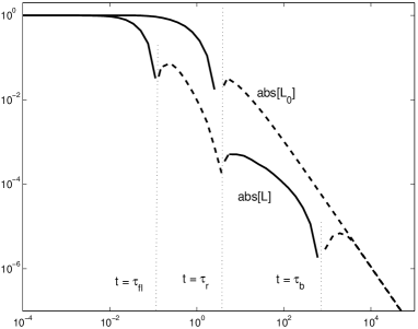
FIG. 1.: The Lagrangian velocity correlation for the subdiffusive transport ( $\overline{\chi}_{\parallel}=0,$ $\overline{\tau}_{c}=\infty).$ $L_{0}(t)$ corresponds to $M\ll 1$ and is given by Eq.(62) and $L(t)$ is the nonlinear result obtained in the presence of magnetic line trapping at large $K_{m}$ ($M=10,$ $\overline{\chi}_{\parallel}=0.1).$ The dashed parts of the two curves represent negative values of the Lagrangian correlations.

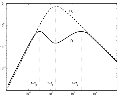
FIG. 2.: The running diffusion coefficient corresponding to the Lagrangian velocity correlations in Figure 1: $D_{0}(t)$ is the integral of $L_{0}(t)$ and is given by Eq.(63) and $D(t)$ is the integral of $L(t)$ and shows the effect of the magnetic line trapping. The normalization constant is $\left(\lambda_{\perp}^{2}\nu\right)M.$

The above evolution of the diffusion appears whenever $\tau_{fl}<\tau_{r},$ and since $\tau_{fl}=M^{-1}$ and $\tau_{r}\approx\overline{\chi}_{\parallel}^{-1/2},$ the condition is $K_{m}>1$ which corresponds to magnetic line trapping. When $\tau_{fl}>\tau_{r}$ (or $K_{m}\ll 1),$ the diffusion coefficient is given by Eq.(63).

We show in the next sections that this rather nontrivial evolution of the running diffusion coefficient leads to anomalous diffusion regimes when a decorrelation mechanism is present.

V Diffusive transport induced by collisional decorrelation

We analyze in this section the effect of the cross-field collisional diffusion ($\overline{\chi}_{\perp}\neq 0)$ starting from the general solution (57)-(59). The stochastic collisional velocity ${\bf\eta}_{\perp}(t)$ in Eq.(3) moves the particles out of the magnetic lines and consequently it has a decorrelation effect leading to diffusive transport. This collisional motion determines a characteristic time, the perpendicular decorrelation time $\tau_{\perp}.$ It is defined by the condition that the collisional diffusion covers the perpendicular correlation length, $2\chi_{\perp}\tau_{\perp}=\lambda_{\perp}^{2},$ and in the units chosen here it is $\tau_{\perp}=(2\overline{\chi}_{\perp})^{-1}.$ The stochastic magnetic field is considered here to be static ($\overline{\tau}_{c}=\infty)$ for a better understanding of the collisional decorrelation.

As in the previous section, a stochastic magnetic field with small Kubo number $K_{m}$ that does not generate stochastic magnetic islands is first considered. We show analytically that the already known results are reproduced by the decorrelation trajectory method. Then the nonlinear case is analyzed and new anomalous diffusion regimes are found. They are determined by the non-linear interaction of the magnetic line trapping with the cross-field collisional diffusion.

In 1979 Kadomtsev and Pogutse [2] derived semi-qualitatively an approximation for the cross-field diffusion coefficient. This approximation is essentially a weak-nonlinearity regime, in which the magnetic field fluctuations are non-chaotic. It will be shown that this diffusion coefficient is obtained from the general equations (57)-(59) provided that $\tau_{r}<\tau_{\perp}<\tau_{fl}.$ This condition is compatible with the relations found in [11] where a detailed study of the diffusion regimes in stochastic magnetic fields for fusion plasmas is presented. In this conditions the ${\bf X}^{S}$-dependence of the average velocity in Eqs.(54), (55) can be neglected and the equations for the decorrelation trajectories are (60) corrected by a factor $n_{\perp}^{2}(t)$ that multiplies the right hand side terms. This leads to the following form of the Lagrangian velocity correlation

$$L_{KP}(t)=n_{\bot}^{2}(t)\,L_{0}(t),$$ (68)

where $L_{0}(t)$ is the subdiffusive Lagrangian velocity autocorrelation defined in Eq. (62). Because of the factor $n_{\bot}^{2}(t)$, the integral of $L_{KP}(t)$ no longer vanishes, and yields a finite diffusion coefficient, $D_{KP}$. It can be estimated analytically by using a step approximation of the function $n_{\bot}(t)$

$$n_{\bot}(t)\cong\left\{\begin{array}[]{c}1,\;\;\;t<\tau_{\perp}\\ 0,\;\;\;\;t>\tau_{\perp}\end{array}\right.$$ (69)

It then follows that the diffusion coefficient is approximated as:

$$D_{KP}\cong\int_{0}^{\tau_{\perp}}dt\,L_{0}(t)=-\int_{\tau_{\perp}}^{\infty}dt\,L_{0}(t)$$ (70)

because the integral of $L_{0}(t)$ from $t=0$ to infinity is zero. Using the very simple asymptotic form of $L_{0}(t)$ [obtained from Eq.(62) for $\tau>\tau_{r}$], the integral can be calculated analytically and one obtains (going to dimensional quantities)

$$D_{KP}\cong\beta^{2}\,\frac{\lambda_{\|}}{\lambda_{\bot}}\sqrt{\chi_{\|}\,\chi_{\bot}}$$ (71)

which is the well-known Kadomtsev-Pogutse formula.

When the time of flight $\tau_{fl}$ is smaller than the decorrelation time $\tau_{\bot},$ the space dependence of the magnetic field fluctuations cannot be neglected. It leads to stochastic magnetic islands. In the presence of a perpendicular collisional diffusivity the decorrelation trajectories obtained from Eq.(55) are not more closed curves. However, trajectory winding can still be observed for some range of the parameters that define the subensembles. This means that the process of generation of stochastic magnetic island and of magnetic line trapping still exists. Compared to the decorrelation trajectories obtained with $\chi_{\perp}=0,$ these trajectories saturate faster and perform a smaller number of rotations. They still turn back at the maximum of the function $\tau(t)$ which shows that the parallel trapping determined by the parallel collisional motion still exists. But due to the cross field collisional diffusion, these two trapping processes are only approximate or temporary. The perpendicular diffusion $\chi_{\bot}$ produces a releasing effect both for perpendicular and parallel components of particle motion. The asymptotic values of the decorrelation trajectories are not concentrated in the origin (as for $\chi_{\bot}=0)$ but spread in the $(X,Y)$ plane. Consequently, a finite value of the asymptotic diffusion coefficient yields from Eq.(58).

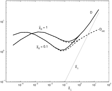
FIG. 3.: The asymptotic diffusion coefficient as a function of $\overline{\chi}_{\perp}.$ The total diffusion coefficient $D$ (continuous lines) is compared with the direct collisional contribution $\overline{\chi}_{\perp}$ (dotted line) and with the interaction term $D_{int}$ (dashed lines) for two values of $\overline{\chi}_{\parallel}.$ The normalization constant is $\lambda_{\perp}^{2}\nu,$ $M=10$ and $\overline{\tau}_{c}=\infty.$

The asymptotic diffusion coefficient is determined from Eq.(58) using the numerical code we have developed. Some results are presented in Figure 3 where the asymptotic value of $D(t)$ is represented as a function of $\overline{\chi}_{\perp}.$ The two components $D_{int}$ and $\overline{\chi}_{\perp}$ are also represented. One can see that at small collisional diffusion $\overline{\chi}_{\perp}\ll 1$, the non-linear interaction term largely dominates the collisional term while at large collisional diffusion $\overline{\chi}_{\perp}\gtrsim 1,$ the nonlinear term is only a correction to $\overline{\chi}_{\perp}.$ Thus, the subdiffusive transport appearing at $\overline{\chi}_{\perp}=0$ is transformed by a small collisional cross field diffusion into a diffusive transport with a diffusion coefficient that can be several orders of magnitude larger than $\overline{\chi}_{\perp}.$ The dependence of the diffusion coefficient on $\overline{\chi}_{\perp}$ is rather nontrivial. There is at very small $\overline{\chi}_{\perp}$ an increase of $D$ up to a maximum which corresponds to $\tau_{\perp}\cong\tau_{b}.$ Then, at larger $\overline{\chi}_{\perp},$ the nonlinear interaction of the parallel and perpendicular trapping with the collisional decorrelation generates a strange transport regime, in which the effective diffusion coefficient decreases as the collisional diffusion $\overline{\chi}_{\perp}$ increases. A minimum of $D$ is obtained when $\overline{\chi}_{\perp}$ determines a decorrelation time of the order of the return time of the parallel motion, $\tau_{\perp}\cong\tau_{r}.$ At larger $\overline{\chi}_{\perp}$ (when $\tau_{\perp}<\tau_{r}),$ the nonlinear contribution $D_{int}$ increases again with the increase of $\overline{\chi}_{\perp}$ but this contribution begins to be comparable and eventually negligible compared to the collisional diffusion coefficient.

We note that the above results obtained with the decorrelation trajectory method are not similar with the heuristic estimation of the asymptotic diffusion coefficient of Rechester and Rosenbluth [1]. This is possibly due to the fact that the trapping of the magnetic lines, which is profoundly implied in the above results, is neglected in the estimation [1] and also in the more detailed calculations presented in [10]. This estimation is based on the process of exponential increase of the average distance between two magnetic lines in a chaotic magnetic field, represented by the Kolmogorov length. The estimation of this length taking into account the trapping of the magnetic lines should be necessary in order to compare the results.

VI Diffusive transport in time-dependent stochastic magnetic fields

In a time-dependent stochastic magnetic field with finite $\tau_{c}$ the configuration of the stochastic field ${\bf b}({\bf x},z,t)$ changes, the magnetic lines move and consequently the perpendicular velocity of the particles is decorrelated leading to diffusive transport. We determine here the diffusion coefficient in such time-dependent fields in the limit of zero Larmor radius, stating from the general solution (57)-(58). The effect of time variation of the stochastic magnetic field on the effective diffusion was previously studied in [17]-[21] but only for weak magnetic turbulence ($K_{m}\ll 1).$ We determine the effect of stochastic island generation appearing in stochastic magnetic fields at $K_{m}>1.$

The decorrelation trajectories obtained from Eqs.(54), (55) are in this case (finite $\tau_{c},$ $\overline{\chi}_{\perp}=0)$ situated on closed paths (except that for $p=0)$. A typical trajectory rotates on the corresponding path, then it stops and turns back. Its velocity decays progressively and eventually the trajectory stops somewhere on its path. This is the modification determined by the time variation of the magnetic field: all decorrelation trajectories stop at a time of the order $\overline{\tau}_{c}.$ Consequently, the running diffusion coefficient saturates. Depending on the relation between the decorrelation time $\overline{\tau}_{c}$ and the three characteristic times of this motion, $\tau_{fl},$ $\tau_{r},$ $\tau_{b}$ (see Fig. 2) several diffusion regimes are obtained.  In time-dependent magnetic fields, at $t<\tau_{c},$ the time evolution of the diffusion coefficient is approximately the same with that obtained for $\overline{\tau}_{c}\rightarrow\infty,$ and later, at $t>\tau_{c},$ $D(t)$ saturates. Thus, the asymptotic diffusion coefficient can be evaluated as

$$\mathrel{\mathop{\lim}\limits_{t\rightarrow\infty}}D(t;M,\overline{\chi}_{\parallel},0,\overline{\tau}_{c})\cong D(\overline{\tau}_{c};M,\overline{\chi}_{\parallel},0,\infty).$$ (72)

using the running diffusion coefficient obtained in the static case. Thus it can be approximating by the value of the running diffusion coefficient for the subdiffusive case at $t=\overline{\tau}_{c}.$  Some results are presented in Figure 4 where the asymptotic diffusion coefficient obtained from Eq.(59)  for finite $\overline{\tau}_{c}$ is compared to the subdiffusive running diffusion coefficient represented in Figure 2. One can see that the approximation (72) is rather good for all values of $\ \overline{\tau}_{c}.$

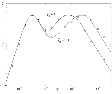
FIG. 4.: The asymptotic diffusion coefficient as a function of $\overline{\tau}_{c}$ for $\overline{\chi}_{\parallel}=0.1$ (circles) and $\overline{\chi}_{\parallel}=1$ (stars). The continuous lines represent the running diffusion coefficient as a function of $t$ for the subdiffusive transport corresponding to static magnetic fields ($\overline{\tau}_{c}=\infty).$ The normalization constant is $\left(\lambda_{\perp}^{2}\nu\right)M^{2}$, $M=10,$ $\overline{\chi}_{\perp}=0.$

The following diffusion regimes can be observed in Figure 4, in the nonlinear conditions when stochastic magnetic islands are generated ($\tau_{fl}<\tau_{r},$ or $K_{m}>1).$ The quasilinear regime at small correlation times ($\overline{\tau}_{c}<\tau_{fl}$) with $D_{0}\approx M^{2}\overline{\tau}_{c}$ is characterized by a fast time-variation which prevents trajectory trapping. At larger correlation times ($\tau_{fl}<\overline{\tau}_{c}<\tau_{r})$ the stochastic magnetic islands can be generated before the stochastic magnetic field changes and the parallel motion is ballistic. In these conditions the diffusion regime is similar to that described in [16] for the electrostatic turbulence: the diffusion coefficient decreases with the increase of $\overline{\tau}_{c}.$ A minimum of the diffusion coefficient appears at $\overline{\tau}_{c}\cong\tau_{r},$ followed by an anomalous increase determined by the interaction of the parallel trapping with the magnetic line trapping which generates correlation of the Lagrangian velocities. At very large correlation times ($\overline{\tau}_{c}>\tau_{b})$ the diffusion coefficient decreases as $D\approx K_{m}^{2}\overline{\tau}_{c}^{-1/2}\overline{\chi}_{\parallel}^{1/2}.$ We note that the regimes obtained for $\overline{\tau}_{c}<\tau_{fl}$ and for $\overline{\tau}_{c}>\tau_{b}$ are similar with those reported in [17], [18]. But instead of the plateau found there at intermediary $\overline{\tau}_{c},$ we obtain here a more complicated behavior. This is the effect of stochastic magnetic island generation: it leads to the decrease of the effective diffusion coefficient with the increase of $\overline{\tau}_{c}$ when the parallel motion is ballistic and, on the contrary, to the increase of $D$ with the increase of $\overline{\tau}_{c}$ when the parallel motion is diffusive.

VII Conclusions

We have studied here the transport of collisional particles in stochastic magnetic fields using the decorrelation trajectory method. We have derived analytical expressions for the running diffusion coefficient and for the Lagrangian velocity correlation in terms of a set of deterministic trajectories. They are defined in subensembles of the realizations of the stochastic field as solution of differential (Hamiltonian) equations that depend on the given Eulerian correlation of the stochastic potential. They are approximations of the subensemble average trajectories and represent the dynamics of the decorrelation of the Lagrangian velocity. Since in general the equations for the decorrelation trajectories cannot be solved analytically, a computer code was developed for determining the running diffusion coefficient for arbitrary values of the four parameters of this problem and for given Eulerian correlation of the potential.

We have shown that this rather complicated triple stochastic process is characterized by two kinds of trajectory trappings and contains two decorrelation mechanisms. The latter are produced by the collisional cross field diffusion $\overline{\chi}_{\perp}$ and by the time variation of the stochastic magnetic field.

One of the trapping processes concerns the parallel motion and is determined by collisions which constrain the particles to return in the already visited places with probability one. This parallel trapping leads to a subdiffusive transport in the absence of a decorrelation mechanism. This already known process is recovered by our method. The second kind of trapping concerns the magnetic lines which at $K_{m}>1$ wind around the extrema of the vector potential generating self-consistently magnetic islands. The effects of the magnetic line trapping in the presence of particle collisions is studied for the first time. We show that in the absence of a decorrelation mechanism, the stochastic magnetic islands determine a transitory decay of the running diffusion coefficient $D(t)$ appearing at $t$ in the interval $(\tau_{fl},\;\tau_{r}),$ i.e. before the parallel trapping is effective. The simultaneous action of both trapping processes determine a nonlinear built up of Lagrangian velocity correlation and eventually the parallel motion washes out the effect of the magnetic line trapping. Consequently, the asymptotic behavior of the running diffusion coefficient is exactly the same as in the quasilinear conditions when the stochastic magnetic field does not generate magnetic islands.

The effect of the two decorrelation mechanisms is afterwards studied. We show that the effective diffusion coefficient and its dependence on the parameters results from a competition between the trapping and the decorrelation processes and more precisely from the temporal ordering of the characteristic times of these processes. Each one of the two decorrelation mechanisms leads to the already known diffusion laws when the stochastic magnetic islands are not present ($K_{m}\ll 1).$ Their presence (at $K_{m}>1)$ produces a complicated nonlinear interaction between the three stochastic processes which determines new scaling laws of the diffusion coefficient. They appear when the decorrelation time is longer than the flight time $\tau_{fl}$ but smaller than the correlation built up time $\tau_{b}.$ The first condition ensures the magnetic islands generation and the second prevents the elimination of their trapping effect by the parallel collisional motion. A particularly interesting regime is obtained for collisional decorrelation and consists of an effective diffusion coefficient that decreases when the collisional perpendicular diffusion increases (Fig. 3).

This rather complex dependence of the diffusion coefficients on the plasma parameters can be used in experiments for controlling the transport. Even without changing the characteristics of the stochastic magnetic field, the diffusion coefficient can be strongly influenced by the parameters which describe particle collisions. A  minimum of the diffusion coefficient was obtained for decorrelation times of the order of the average return time for the parallel motion.

Acknowledgement 1

This work has benefited of the NATO Linkage Grant PST.CLG.977397 which is acknowledged.

REFERENCES

- [1] A. B. Rechester and M. N. Rosenbluth, Phys. Rev. Lett. 40, 38 (1978).
- [2] B. B. Kadomtsev and O. P. Pogutse, in Plasma Physics and Controlled Nuclear Fusion Research 1978, Proceedings of the Seventh International Conference, Innsbruck (International Atomic Energy Agency, Vienna, 1979).
- [3] R. J. Jokipii and E. N. Parker, Astrophys. J. 155, 777 (1969).
- [4] P. H. Diamond, T. H. Dupree, and D. J. Tetreault, Phys. Rev. Lett. 45, 562 (1980).
- [5] J. A. Krommes, C. Oberman and R. G. Kleva, J. Plasma Phys. 30, 11 (1983).
- [6] M. B. Isichenko, Plasma Phys. and Controlled Fusion 33, 795 (1991).
- [7] R. B. White and Y. Wu, Plasma Phys. Controlled Fusion 35, 595 (1993).
- [8] J. R. Myra, P. J. Catto, H. E. Mynick, and D. E. Duvall, Phys. Fluids B 5, 1160 (1993).
- [9] F.Spineanu, M.Vlad, J.H.Misguich, Journal of Plasma Physics 51, 113 (1994).
- [10] Hai-Da Wang, M. Vlad, E. Vanden Eijnden, F. Spineanu, J. H. Misguich and R. Balescu, Phys. Rev. E 51, 4844 (1995).
- [11] J. H. Misguich, M. Vlad, F. Spineanu and R. Balescu, Comments Plasma Phys. Controlled Phys. 17, 45 (1995).
- [12] M.Vlad, F. Spineanu, J. H. Misguich, and R. Balescu, Phys. Rev. E 54, 791 (1996).
- [13] M. Vlad, J.-D. Reuss, F. Spineanu and J. H. Misguich, Journal of Plasma Phys. 59, 707 (1998).
- [14] R. Balescu, H.-D. Wang, and J. H. Misguich, Phys. Plasmas 1, 3826 (1994).
- [15] M. Vlad, F. Spineanu, J. H. Misguich and R. Balescu, Phys. Rev. E 58, 7359 (1998) .
- [16] M. Vlad, F. Spineanu, J. H. Misguich, and R. Balescu, Phys. Rev. E 61, 3023 (2000).
- [17] J. H. Misguich, M.Vlad, F. Spineanu, and R. Balescu, Report EUR-CEA-FC-1556 (1995).
- [18] M.Vlad, F. Spineanu, J. H. Misguich, and R. Balescu, Phys. Rev. E 53, 5302 (1996).
- [19] M. Coronado, E. J. Vitel, and A. Akcasu, Phys. Fluids B 4, 3955 (1992).
- [20] A. Thyagaraja, I. L. Robertson, and F. A. Haas, Plasma Phys. and Controlled Fusion 27, 1217 (1985).
- [21] H. Ludger, Phys. Fluids B 5, 3551 (1993).