A Gaussian-optical Approach to Stable Periodic Orbit Resonances of Partially Chaotic Dielectric Micro-cavities

Abstract

The quasi-bound modes localized on stable periodic ray orbits of dielectric micro-cavities are constructed in the short-wavelength limit using the parabolic equation method. These modes are shown to coexist with irregularly spaced “chaotic” modes for the generic case. The wavevector quantization rule for the quasi-bound modes is derived and given a simple physical interpretation in terms of Fresnel reflection; quasi-bound modes are explictly constructed and compared to numerical results. The effect of discrete symmetries of the resonator is analyzed and shown to give rise to quasi-degenerate multiplets; the average splitting of these multiplets is calculated by methods from quantum chaos theory.

I Introduction

There is currently a great deal of interest in dielectric micro-cavities which can serve as high-Q resonators by confining light on the basis of multiple reflections from a boundary of dielectric mismatch campillo_book ; yokoyama1 ; nobel ; science ; nature . Such resonators have been used to study fundamental optical physics such as cavity quantum electrodynamics campillo1 ; lin1 and have been proposed and demonstrated as the basis of both active and passive optical components vahala1 ; little1 . Of particular interest in this work are dielectric micro-cavity lasers which have already been demonstrated for a wide variety of shapes: sphereschang3 , cylinders campillo_book , squares poon1 , hexagons braun1 , and deformed cylinders and spheres (asymmetric resonant cavities nobel - ARCs)science ; mekis ; nockel1 ; gornik1 ; chang1 ; rex1 . The work on ARC micro-cavity lasers has shown the possibility of producing high power directional emission from such lasers, which lase in different spatial mode patterns depending on the index of refraction and precise shape of the boundary. For example modes based on stable periodic ray orbits with bow-tie science and triangular geometry rex_thesis have been observed, as well as whispering gallery-like modes chang1 ; rex_thesis which are not obviously related to any periodic ray orbit. In addition a periodic orbit mode can be selected for lasing even if it is unstable rex1 ; gmachl1 ; sblee1 ; due to the analogy to quantum wavefunctions based on unstable classical periodic orbits, such modes have been termed “scarred” heller1 . There is at present no quantitative understanding of the mode selection mechanism in ARCs and theory has tended to work backwards from experimental observations; however the passive cavity solutions have been found to explain quite well the observed lasing emission patterns. The formal analogy between ARCs and the problem of classical and quantum billiards has given much insight into their emission properties campillo_book ; nobel . For example it was predicted and recently observed that polymer ARCs of elliptical shape (index $n=1.49$) have dramatically different emission patterns from quadrupolar shaped ARCs with the same major to minor axis ratio harald1 . The difference can be fully understood by the different structure of the phase space for ray motion in the two cases, the ellipse giving rise to integrable ray motion and the quadrupole to partially chaotic (mixed) dynamics. Resonators are of course open systems for which radiation can leak out to infinity. In the discussion of the ray-wave correspondence immediately following we neglect this leakage assuming only perfect specular reflection of light rays at the dielectric boundary. However the theory of ARCs nobel ; nature includes these effects and they will be treated when relevant below.

As is well-known, the geometric optics of a uniform dielectric region with perfectly reflecting boundaries is formally analogous to the problem of a point mass moving in a billiard and hence we may use the terminology of Hamiltonian dynamics to describe ray motion in the resonator. As discussed below, we shall specialize to cylindrical geometries in which the relevant motion will be in the the plane transverse to the axis, hence we focus on two-dimensional billiards. The quadrupole billiard is an example of a generic deformation of the circle or cylinder in that it is smooth and analytic and does not preserve any constant of motion. (Motion in the circle of course conserves angular momentum and motion in a closed elliptical cavity conserves a generalized angular momentum, the product of the instantaneous angular momenta with respect to each focus berry2 ). A generic deformation such as the quadrupole will lead to a phase space for ray motion which has three types of possible motion (depending on the choice of initial conditions): oscillatory motion in the vicinity of a stable periodic ray orbit, chaotic motion in regions associated with unstable periodic ray orbits, and marginally stable motion associated with families of quasi-periodic orbits (motion on a so-called KAM torus). To elucidate the structure of phase space it is conventional to plot a number of representative trajectories in a two-dimensional cut through phase space, called the surface of section (Fig. 1). For our system the surface of section corresponds to the boundary of the billiard and the coordinates of the ray are the polar angle $\phi$ and the angle of incidence $\sin\chi$ at each bounce. The three types of motion described above are illustrated for the quadrupole billiard in Fig. 1 both in phase space and in real space.

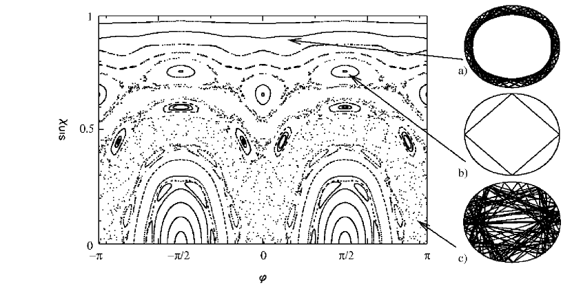
Figure 1: Surface of section illustrating the different regions of phase space for a closed quadrupole billiard with boundary given by $r(\phi)=R(1+\epsilon\cos 2\phi)$ for $\epsilon=0.072$. Real-space ray trajectories corresponding to each region are indicated at left: a) A quasi-periodic, marginally stable orbit. b) A stable four-bounce “diamond” periodic orbit (surrounded by stability “islands” in the SOS) c) A chaotic ray trajectory. Orbits of type (b) have associated with them regular gaussian solutions as we will show below.

It has been shown robnik1 that the solutions of the wave equation for a generic shape such as the quadrupole can be classified by their association with these three different kinds of motion. The ray-mode (or wave-particle) correspondence becomes stronger as we approach the short-wavelength (semi-classical) limit, which in this work is defined by $kl\gg 1$ where $k$ is the wavevector and $l$ is a typical linear dimension of the resonator, e.g. the average radius. The modes associated with quasi-periodic families can be treated semiclassically by eikonal methods of the type introduced, e.g. by Keller keller1 , and referred to in its most general form as EBK (Einstein-Brillouin-Keller) quantization. The individual modes associated with unstable periodic orbits and chaotic motion cannot be treated by any current analytic methods (although the density of states for a chaotic system can be found by a sophisticated analytic method based on Gutzwiller’s Trace Formula gutz_book ). Finally, the modes associated with stable periodic orbits can be treated by generalizations of gaussian optics and will be the focus of the current work.

If a mode is found by numerical solution, its interpretation in terms of the ray phase space can be determined with reasonable accuracy by means of the Husimi projection onto the phase space (see Fig. 2), although it is well-known that for $kl$ not much greater than unity the exact solutions tend to smear out in the phase space over regions of order $1/kl$ and do not correspond very closely to specific classical structures. For a closed generic ARC the full spectrum will look highly irregular (see Fig. 3(a)), but contained in the full spectrum will be regular sequences associated with tori and stable periodic orbits (Fig. 3(b)). The stable periodic orbit modes will give the simplest such sequences consisting of two different constant spacings, one associated with the longitudinal quantization of the orbit (free spectral range) and the other associated with transverse excitations. In the example of Fig. 3 the imbedded regular spectrum is due to the stable “bow-tie” orbit. The regular portion of the spectrum is extracted by weighting each level by the overlap of its Husimi function with the islands corresponding to the stable periodic orbit in the surface of section. Clearly, hidden within this complex spectrum are simple regular mode sequences of the type familiar from Gaussian optics. In the current work we show how to calculate the resonant energies and spatial intensity patterns of such modes associated with arbitrary stable periodic ray orbits for both the ideal closed resonator and a dielectric resonator of the same shape with arbitrary dielectric mismatch $n$. We shall refer to these as periodic orbit modes or PO modes.

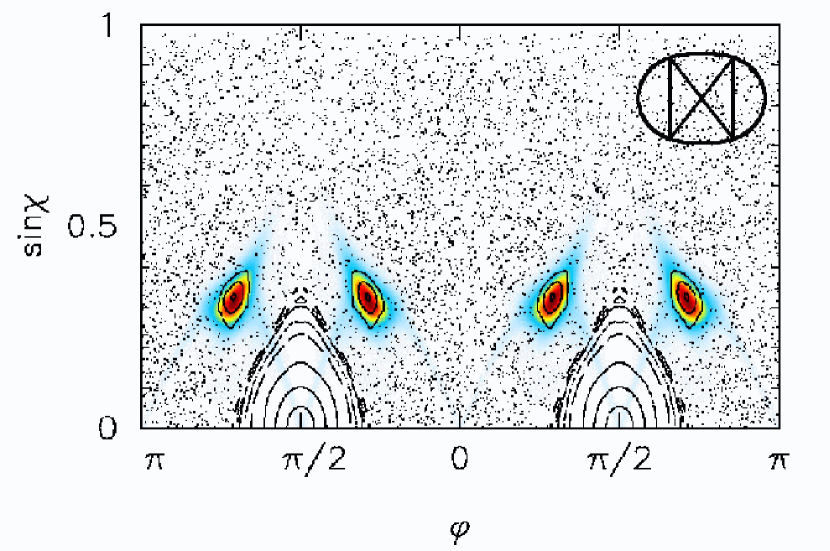
Figure 2: Black background gives the surface of section for the quadrupole at $\epsilon=0.17$ for which the four small islands correspond to a stable bow-tie shaped orbit (inset). A numerical solution of the Helmholtz equation for this resonator can be projected onto this surface of section via the Husimi transform [27] and is found to have high intensity (in false color scale) precisely on these islands, indicating that this is a mode associated with the bow-tie orbit.

In the case of the open resonator, the modes have a width which can be expressed as a negative imaginary part of k, and some of the PO modes may be so broad (short-lived) that they would not appear as sharp spectral lines. Within the gaussian-optical theory we present below that this width is entirely determined by Fresnel reflection at the interface and would be zero for a periodic orbit which has all bounces above the total internal reflection condition, but would be quite large for a periodic orbit, such as the two-bounce Fabry-Perot orbit, which has normal incidence on the boundary. An exact solution must find a non-zero width for all PO modes, due to evanescent leakage across a curved interface, even if all the bounces satisfy the total internal reflection condition.

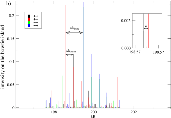
Figure 3: (a) Vertical lines indicate wavevectors of bound states of the closed quadrupole resonator for $\epsilon=0.17$; no regular spacings are visible. (b) Spectrum weighted by overlap of the Husimi function of the solution with the bow-tie island as in Fig. 2. Note the emergence of regularly spaced levels with two main spacings $\Delta k_{long}$ and $\Delta k_{trans}$. These spacings, indicated by the arrows, are calculated from the length of the bow-tie orbit and the associated Floquet phase (see section II.4 below). The color coding corresponds to the four possible symmetry types of the solutions (see section IV below). In the inset is a magnified view showing the splitting of quasi-degenerate doublets as discussed in section IV.3. Note the pairing of the $(+,+)$ and $(+,-)$ symmetry types as predicted in section IV.2. The different symmetry pairs alternate every free spectral range ($\Delta k_{long}$).

Another limitation of the gaussian theory of stable PO modes is that it predicts exactly degenerate modes when the associated orbit has discrete symmetries, even in cases for which a group-theoretic analysis shows that there can be no exact symmetries (this is the case, for example in the quadrupole). Instead the exact solutions will have some integer quasi-degeneracy in which the spectrum consists of nearly degenerate multiplets, whose multiplicity depends in detail on the particular PO mode. This point is illustrated by the inset to Fig. 3(b). We will show below how to calculate the multiplicity of these quasi-degeneracies for a given PO and introduce a theoretical approach to estimate the size of the associated splittings.

II Gaussian optical approach to the closed cavity

The quantization of electromagnetic modes within dielectric bodies enclosed by metallic boundaries, including the case of arbitrary index variation inside the resonator and three-dimensions has been treated before in the literature babic_book . However the generality of the treatment makes it difficult to extract simple results of use to researchers working with uniform dielectric optical micro-cavities; more importantly all the work of which we are aware focuses on the case of Dirichlet boundary conditions corresponding to perfect reflection at the boundary. Perfect reflection of course leads to true bound states. In the next section we show how to generalize these results to the correct boundary conditions at a dielectric interface and hence for the case of quasi-bound as opposed to bound states. However, first, in this section we develop the formalism for the closed case which we will generalize to the case of interest. In all of this work we will specialize to the case of two dimensions, corresponding to an infinite dielectric cylinder with an arbitrary cross-section in the transverse plane (see Fig. 4) with the condition $k_{z}=0$. To conform with conventions introduced below we will refer to the two-dimensional coordinate system as $(X,Z)$. In this case the TM and TE polarizations separate and we have a scalar wave equation with simple continuity conditions at the boundary for the electric field (for TM) or magnetic field (for TE). For the closed case (for which the field is zero on the boundary) we can set the index $n=1$ and work simply with the Helmholtz equation.

\psfrag{bb}{$\partial D$}\includegraphics[width=260.17464pt]{cylinder.eps}

Figure 4: Illustration of the reduction of the Maxwell equation for an infinite dielectric cylinder to the 2D Helmholtz equation for the TM case (E field parallel to axis) and $k_{z}=0$.

Consider the solutions $E(X,Z)$ of the Helmholtz equation in two dimensions:

$$\left(\nabla^{2}+k^{2}\right)E=0$$ (1)

This solution is assumed to be defined in a bounded two dimensional domain $D$, with a boundary $\partial D$ on which $E=0$, leading to discrete real eigenvalues $k$. We are interested in a subset of these solutions for asymptotically large values of $k$ for which the eigenfunctions are localized around stable periodic orbits(POs) of the specularly reflecting boundary $\partial D$.

II.1 The Parabolic equation approximation

The “N-bounce PO”s corresponding to a boundary $\partial D$ are the set of ray orbits which close upon themselves upon reflecting specularly N times. The shape of the boundary defines a non-linear map from the incident angle and polar angle at the $m^{th}$ bounce $(\phi_{m},\sin\chi_{m})$ to that at the $m+1$ bounce. Typical trajectories of this map are shown in the surface of section plot of Fig. 1. The period-N orbits are the fixed points of the $N^{th}$ iteration of this map. For a given period-N orbit (such as the period four “diamond” orbit shown in Fig. 5), let the length of $m$th segment (“arm”) be $l_{m}$, the accumulated distance from origin be $L_{M}=\sum_{m=1}^{M}~{}l_{m}$, and $L=L_{N}$ be the length of the entire PO. We are looking for modal solutions which are localized around the PO and decay in the transverse direction, hence we express Eq. (1) in Cartesian coordinates $(x_{m},z_{m})$ attached to the PO, where $z_{m}$-axis is aligned with $m$th arm and $x_{m}$ is the transverse coordinate. We also use $z$ to denote the cumulative length along the PO, which varies in the interval $(-\infty,+\infty)$.

\psfrag{bb}{$\partial D$}\includegraphics[width=216.81pt]{coordinates.eps}

Figure 5: Coordinate system and variables used in the text displayed for the case of a quadrupolar boundary $\partial D$ and the diamond four-bounce PO. A fixed coordinate system $(X,Z)$ is attached to the origin. The “mobile” coordinate systems $(x_{m},z_{m})$ are fixed on segments of the periodic orbit so that their respective $z$-axes are parallel to the segment, while their origins are set back a distance $L_{m}$ (or $nL_{m}$ for transmitted beam axes), so as to account for zeroth order phase accumulation between successive bounce-points. $\xi_{1},\xi_{2}$ are the common local coordinates at each bounce (index $m$ suppressed). Scaled coordinates are denoted by tildes, e.g. $\tilde{x}_{m}=\sqrt{k}x_{m}$. The coordinate transformations at each bounce $m$ are given by $z_{i}=L_{m}+\xi_{1}\sin\chi_{i}+\xi_{2}\cos\chi_{i}$, $z_{r}=L_{m}+\xi_{1}\sin\chi_{i}-\xi_{2}\cos\chi_{i}$, $z_{t}=nL_{m}+\xi_{1}\sin\chi_{t}+\xi_{2}\cos\chi_{t}$ and $x_{i}=\xi_{1}\cos\chi_{i}-\xi_{2}\sin\chi_{i}$, $x_{r}=\xi_{1}\cos\chi_{i}+\xi_{2}\sin\chi_{i}$, $x_{t}=\xi_{1}\cos\chi_{t}-\xi_{2}\sin\chi_{t}$, where $i,r,t$ refer to the incident, transmitted and reflected solutions.

We write the general solution as:

$$E(X,Z)=\sum_{m=1}^{N}E_{m}(x_{m}(X,Z),z_{m}(X,Z))$$ (2)

where the “local set” $(x_{m},z_{m})$ and the fixed set $(X,Z)$ are related by shifts and rotations (see Fig. 5). Next, in accordance with the parabolic equation approximation babic_book , we assume that the main variation of the phase in z-direction is linear (“slowly varying envelope approximation”) and factor it out:

$$E_{m}(x_{m},z_{m})=u_{m}(x_{m},z_{m})e^{ikz_{m}}$$ (3)

This definition suggests defining the origins of the local coordinates such that $z_{m}=z$ along the PO, and we do so (see Fig. 5).

Next, we insert the solution Eq. (2) into Eq. (1) and using the invariance of the Laplacian, we obtain:

$$\left(\nabla_{m}^{2}+k^{2}\right)E_{m}=0$$ (4)

and the boundary condition translates into

$$E_{m}+E_{m+1}|_{\partial D}=0$$ (5)

Here $\nabla_{m}$ is the Laplacian expressed in local coordinate system. This reduction is possible as long as the solutions are well-localized, and the bounce points of the PO are well-separated (with respect to $k^{-1}$), even if the PO were to self-intersect. These assumptions will be justified by the ensuing construction.

Dropping for the moment the arm index, we will focus on Eq. (4). Inserting Eq. (3), we arrive at

$$u_{xx}+u_{zz}+2iku_{z}=0$$ (6)

The basic assumption of the method is that after removing phase factor $\exp[ikz]$ which varies on the scale of the wavelength $\lambda$, the $z$-dependence of $u$ is slow, i.e. $u_{z}\sim u/l,u_{zz}\sim u/l^{2}$, where $l$ is a typical linear dimension associated with the boundary, e.g. a chord length of the orbit or the curvature at a bounce point. In the semiclassical limit $l\gg\lambda$. The transverse ($x$) variation of $u$ on the other hand is assumed to occur on a scale $\sqrt{l\lambda}$, intermediate between the wavelength and the cavity scale, $l$; hence the transverse variation of $u(x,z)$ is much more rapid than its longitudinal variation. This motivates us to introduce the scaling $\tilde{x}=\sqrt{k}x$ to treat this boundary layer, which leads to

$$u_{\tilde{x}\tilde{x}}+\frac{1}{k}u_{zz}+2iu_{z}=0.$$ (7)

We can now neglect the $u_{zz}$ term due to the condition $kl\gg 1$, and obtain a partial differential equation of parabolic type:

$${\cal L}\;u(\tilde{x},z)=0$$ (8)

where ${\cal L}=\partial_{\tilde{x}}^{2}+2i\partial_{z}$. Next, we make the ansatz

$$u(x,z)=c\>A(z)\exp{\left[\frac{i}{2}\Omega(z)\tilde{x}^{2}\right]}$$ (9)

Inserting Eq. (9) into Eq. (8) and requiring it to be satisfied for all $x$, we obtain the relations

$$\Omega^{2}+\Omega^{\prime} = 0$$ (10)

$$A\Omega+2A^{\prime} = 0$$ (11)

Here and in the rest of the text we will use primes as a shorthand notation for a $z$-derivative. Next, making the substitution

$$\Omega=\frac{Q^{\prime}(z)}{Q(z)}$$ (12)

we obtain

$$Q^{\prime\prime} = 0$$ (13)

$$\frac{Q^{\prime}}{Q}+2\frac{A^{\prime}}{A} = 0$$ (14)

Note that Eq. (13) is the Euler equation for ray propagation in a homogeneous medium with general solution $Q(z)=\alpha z+\beta$; we will be able to interpret $Q(z)$ below as describing a ray nearby the periodic orbit with relative angle and intercept determined by $\alpha,\beta$.

II.2 Boundary Conditions

Having found the general solution of Eq. (8) along one segment of the periodic orbit we must impose the boundary condition Eq. (5) in order to connect solutions in successive segments. Writing out this condition:

$$\frac{c_{m}}{\sqrt{Q_{m}(z_{m})}}\exp{\left(ikz_{m}+\frac{i}{2}\Omega(z_{m})\tilde{x}_{m}^{2}\right)}+\frac{c_{m+1}}{\sqrt{Q_{m+1}(z_{m+1})}}\exp{\left(ikz_{m+1}+\frac{i}{2}\Omega(z_{m+1})\tilde{x}_{m+1}^{2}\right)}|_{\partial D}=0$$

This equation must be satisfied on an arc of the boundary of length $\sim\sqrt{\lambda l}$ around the reflection point. Since this length is much smaller than $l$ we can express this arc on the boundary $\partial D$ as an arc of a circle of radius $\rho$ (the curvature at the reflection point). We express the boundary condition in a (scaled) common local coordinate system for the incident and reflected fields $(\tilde{\xi}_{1},\tilde{\xi}_{2})$ pointing along the tangent and the normal at the bounce point (see Fig. 5). Because the boundary condition must be satisfied on the entire arc it follows the phases of each term must be equal,

$$k\left(l_{m}+\frac{1}{\sqrt{k}}\tilde{\xi}_{1}\sin\chi_{m}-\frac{1}{k}\frac{\tilde{\xi}_{1}^{2}}{2\rho_{m}}\cos\chi_{m}\right)+\frac{1}{2}\frac{Q^{\prime}_{m}}{Q_{m}}\left(\tilde{\xi}_{1}\cos\chi_{m}+\frac{1}{k}\frac{\tilde{\xi}_{1}^{2}}{2\rho_{m}}\sin\chi_{m}\right)^{2}=$$

$$k\left(l_{m}+\frac{1}{\sqrt{k}}\tilde{\xi}_{1}\sin\chi_{m}+\frac{1}{k}\frac{\tilde{\xi}_{1}^{2}}{2\rho_{m}}\cos\chi_{m}\right)+\frac{1}{2}\frac{Q^{\prime}_{m+1}}{Q_{m+1}}\left(\tilde{\xi}_{1}\cos\chi_{m}+\frac{1}{k}\frac{\tilde{\xi}_{1}^{2}}{2\rho_{m}}\sin\chi_{m}\right)^{2}$$

and there is a amplitude condition as well,

$$\frac{c_{m}}{\sqrt{Q_{m}(L_{m})}}+\frac{c_{m+1}}{\sqrt{Q_{m+1}(L_{m})}}=0$$

Here, we assume that $\tilde{\xi}_{1}=O(1)$, and we will carry out the solution of these equations to $O(1/\sqrt{k})$. Note that, it is sufficient to take $Q(z)|_{\partial D}\approx Q(l_{m})$, at this level. In each segment we have three constants which determine our solution: $c_{m},\alpha_{m},\beta_{m}$ (where $Q_{m}(z)=\alpha_{m}z+\beta$); however due to its form our solution is uniquely determined by the two ratios $\beta_{m}/\alpha_{m},c_{m}/\sqrt{\alpha_{m}}$. Therefore we have the freedom to fix one matching relation for the $Q_{m}$ by convention, which then determines the other two uniquely. To conform with standard definitions we fix $Q_{m+1}=Q_{m}$, then the amplitude and phase equality conditions give the relations:

$$\left(\begin{array}[]{c}Q_{m+1}\\ Q^{\prime}_{m+1}\end{array}\right)=\left(\begin{array}[]{cc}1&0\\ -\frac{2}{\rho_{m}\cos\chi_{m}}&1\end{array}\right)\left(\begin{array}[]{c}Q_{m}\\ Q^{\prime}_{m}\end{array}\right)\equiv{\cal R}_{m}\left(\begin{array}[]{c}Q_{m}\\ Q^{\prime}_{m}\end{array}\right)$$ (15)

and

$$C_{m+1}=e^{-i\pi}C_{m}$$ (16)

Here we always choose the principal branch of $\sqrt{Q}$. These conditions allow us to propagate any solution through a reflection point via the reflection matrix ${\cal R}_{m}$ and Eq. (16). Note that with these conventions the reflection matrix is precisely the standard “ABCD” matrix of ray optics for reflection at arbitrary incidence angle (in the tangent plane) from a curved mirror siegman_book . It follows that $Q_{m}$ and $Q_{m+1}$ can be interpreted as the transverse coordinates of the incident and reflected rays with respect to the PO, and that then Eq. (15) describes specular ray reflection at the boundary, if the non-linear dynamics is linearized around the reflection point.

II.3 Ray dynamics in phase space

To formalize the relation to ray propagation in the paraxial limit we define the ray position coordinate to be $Q$ and the conjugate momentum $P=Q^{\prime}$, with $z$ playing the role of the time. Let’s introduce the column-vector $(\stackrel{{\scriptstyle\scriptstyle\>Q\>}}{{{}_{\scriptstyle\>P\>}}})$. The “fundamental matrix” $\Pi$ is the matrix obtained by two such linearly independent vectors

$$\Pi=\left(\begin{array}[]{cc}Q_{1}&Q_{2}\\ P_{1}&P_{2}\end{array}\right)$$ (17)

where the linear independence, as expressed by the Wronskian condition $W(Q^{\prime},Q)\neq 0$ reduces to $\mbox{det}\Pi\neq 0$. Then, for example, the Euler equation Eq. (13) in each arm can be expressed as

$$\frac{d\Pi}{dz}={\cal JH}\,\Pi$$ (18)

where ${\cal H}=(\>\stackrel{{\scriptstyle\scriptstyle 0\>1}}{{{}_{\scriptstyle 0\>0}}}\>)$ and ${\cal J}=(\>\stackrel{{\scriptstyle\scriptstyle 1\mbox{\ }0}}{{{}_{\scriptstyle 0-\!1}}}\>)$. It’s straightforward to show that $\mbox{det}\Pi$ is a constant of motion. To take into account the discreteness of the dynamics in a natural manner, we will introduce “coordinates” for the ray, represented by a $z$-independent column vector $h$. Any ray of the $m$th arm in the solution space of Eq. (13) can then be expressed by a z-independent column vector $h_{m}$

$$\left(\begin{array}[]{c}Q(z)\\ P(z)\end{array}\right)=\Pi(z)h_{m}$$ (19)

We will choose $\Pi(z)=(\>\stackrel{{\scriptstyle\scriptstyle 1\>z}}{{{}_{\scriptstyle 0\>1}}}\>)$, so that $\Pi^{-1}(z)=\Pi(-z)$. Then if $Q_{m}(z)=\alpha_{m}z+\beta_{m}$, we have $h_{m}=(\stackrel{{\scriptstyle\scriptstyle\>\beta_{m}\>}}{{{}_{\scriptstyle\>\alpha_{m}\>}}})$. In this notation, propagation within each arm (i.e. $z+l<L_{m}$ where $L_{m-1}<z<L_{m}$) is induced by the ‘propagator’ $\Pi$

$$\left(\begin{array}[]{c}Q_{m}(z+l)\\ P_{m}(z+l)\end{array}\right)=\Pi(l)\left(\begin{array}[]{c}Q_{m}(z)\\ P_{m}(z)\end{array}\right)$$ (20)

which is the “ABCD” matrix for free propagation siegman_book . Thus, for example $z\rightarrow z^{\prime}$ propagation for $L_{m-1}<z<L_{m}<z^{\prime}<L_{m+1}$ is

$$\left(\begin{array}[]{c}Q_{m+1}(z^{\prime})\\ P_{m+1}(z^{\prime})\end{array}\right)=\Pi(z^{\prime}-L_{m}){\cal R}_{m}\Pi(L_{m}-z)\left(\begin{array}[]{c}Q_{m}(z)\\ P_{m}(z)\end{array}\right)$$ (21)

Of special importance is the monodromy matrix, ${\cal M}(z)$, which propagates rays a full round-trip, i.e. by the length $L$ of the corresponding PO and is given by

$${\cal M}(z)=\Pi(z-L_{m-1}){\cal R}_{m-1}\Pi(l_{m-1})\cdots\Pi(l_{m+1}){\cal R}_{m}\Pi(L_{m}-z)$$ (22)

for $L_{m-1}<z<L_{m}$. Note that $l_{m+N}=l_{m}$ and ${\cal R}_{m+N}={\cal R}_{m}$. Although the specific form of ${\cal M}(z)$ depends on the choice of origin, $z$, it is easily shown that all other choices would give a similar matrix and hence the eigenvalues of the monodromy matrix are independent of this choice. We will suppress the argument $z$ below.

II.4 Single-valuedness and quantization

Having determined how to propagate an initial solution $Q,P$ an arbitrary distance around the periodic orbit we can generate a solution of the parabolic equation which satisfies the boundary conditions by an arbitrary initial choice $Q(0),P(0)$. However an arbitrary solution of this type will not reproduce itself after propagation by L (one loop around the PO). Recalling that our solution is translated back into the two-dimensional space $(X,Z)$ by Eq. (2), and that the function $E(X,Z)$ must be single-valued, we must require periodicity for our solutions

$$E(x,z+L)=E(x,z).$$ (23)

We will suppress again the reference to arm index and use the notation $E(x,z)=E_{m}(x_{m},z_{m})$ and $u(x,z)=u_{m}(x_{m},z_{m})$ whenever $L_{m-1}<z<L_{m}$. Since the phase factor in $E$ advances by $\exp[ikL]$ with each loop around the periodic orbit and single-valuedness implies that

$$u(x,z+L)e^{ikL}=u(x,z).$$ (24)

This periodicity condition will only be solvable for discrete values of $k$ and will lead to our quantization rule for the PO modes.

From the form of $u$ in Eq. (9) we see that the phase $\Omega(z)=Q^{\prime}/Q$ will be unchanged if we choose $(Q,P)$ to be an eigenvector $(q_{1},p_{1})),(q_{2},p_{2})$ of the monodromy matrix as in this case the $Q^{\prime}(z+L)=\lambda_{1,2}Q^{\prime}(z),Q(z+L)=\lambda_{1,2}Q(z)$ and the ratio $\Omega(z)=\Omega(z+L)$. The monodromy matrix is unimodular and symplectic and its eigenvalues come in inverse pairs, which are either purely imaginary (stable case) or purely real (unstable and marginally stable cases). If the PO is unstable and the eigenvalues are real, then the eigenvectors and hence $\Omega(z)$ are real. But a purely real $\Omega(z)$ means that the gaussian factor in $u(x,z)$ is purely imaginary and the solution does not decay in the direction transverse to the PO, contradicting the initial assumption of the parabolic approximation to the Helmholtz equation. Hence for unstable POs our construction is inconsistent and we cannot find a solution of this form localized near the PO.

On the other hand, for the stable case the eigenvalues come in complex conjugate pairs and the reality of the monodromy matrix then implies that the eigenvectors cannot be purely real and are related by complex conjugation. Therefore we can always construct a gaussian solution based on the eigenvector with $Im{\Omega}>0$ so that there is a negative real part of the gaussian exponent and the resulting solution decays away from the PO. It is easy to check that the range of the decay is $\sim\sqrt{\lambda l}$ as assumed above.

The eigenvectors of the monodromy matrix are sometimes referred to as Floquet rays of the corresponding Euler equation. In a more formal discussion which can be straightforwardly generalized to arbitrary index variation and three dimensions babic_book our condition on the choice of $\Omega$ can be expressed by recalling that the two eigenvectors must generate a constant Wronskian, and we will choose the eigenvector $(q(z),p(z))$ such that

$$pq^{*}-qp^{*}=i.$$ (25)

This condition implies $Im{\Omega}>0$. Note that the overall magnitude of the Wronskian is determined by our choice of normalization of the eigenvectors and is here chosen to be unity.

Having made this uniquely determined choice (up to a scale factor) and using $(\stackrel{{\scriptstyle\scriptstyle\>q(z+L)\>}}{{{}_{\scriptstyle\>p(z+L)\>}}})=e^{i\varphi}(\stackrel{{\scriptstyle\scriptstyle\>q(z)\>}}{{{}_{\scriptstyle\>p(z)\>}}})$ and $c_{m+N}=e^{-i\pi N}c_{m}$ we obtain

$$u(\tilde{x},z+L)=e^{-i\frac{\varphi}{2}-i\pi(N_{\mu}+N)}u(\tilde{x},z)$$ (26)

From Eq. (23) and Eq. (3), we finally obtain the quantization rule for the wavevectors of the bound states of the closed cavity:

$$kL=\frac{1}{2}\varphi+2\pi m+\bmod_{2\pi}[(N+N_{\mu})\pi]$$ (27)

where $m$ is an integer, $N$ is the number of bounces in the PO, $\varphi$ is the Floquet phase obtained from the eigenvalues of the monodromy matrix and $N_{\mu}$ is an integer known as the Maslov index in the non-linear dynamics literature maslov_book . It arises in the following manner. As already noted, the eigenvalues of the monodromy matrix for stable POs are complex conjugate numbers of modulus unity whose phase is the Floquet phase. We can define $\varphi=\mbox{Arg}[\sqrt{q(L)/q(0)}]$, where $\mbox{Arg}[\cdot]$ denotes the principal argument; hence the Floquet phase depends only on $\cal{M}$. However our solution, Eq. (9), involves the square root of $q(z)$ and will be sensitive to the number of times the phase of $q(z)$ wraps around the origin as $z$ goes from zero to $L$. If this winding number (or Maslov index) is called $N_{\mu}$ then the actual phase advance along the PO is $\varphi+2\pi N_{\mu}$; if $N_{\mu}$ is odd this leads to an observable $\pi$ phase shift in the solution not included by simply diagonalizing ${\cal M}$ to find the Floquet phase.

$N_{\mu}$ may be directly calculated by propagating $q(z)$:

$$N_{\mu}=\left[\frac{1}{2\pi i}\int_{0}^{L}d(\ln{q(z)})\right]$$ (28)

where $[\cdot]$ denotes the integer part. There is no simple rule for reading off the Maslov index from the geometry of the PO; however the Maslov index doesn’t affect the free spectral range or the transverse mode spacing.

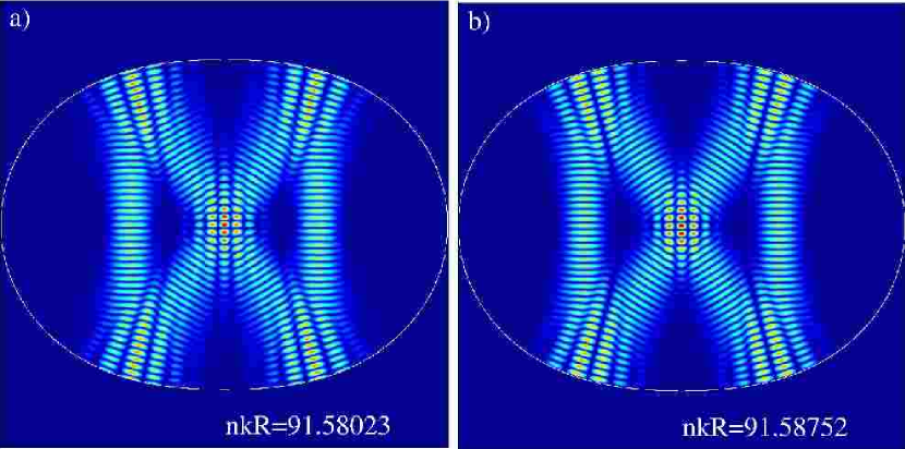
Figure 6: Intensity of the TM solution for a bow-tie mode plotted in a false color scale, (a) calculated numerically and (b) from the gaussian optical theory with parameters $m=100$, $\varphi=2.11391$, $N_{\mu}=1$ and $N=4$. Note the excellent agreement of the quantized values for $kR$ (R is the average radius of the quadrupole).

Except for the Maslov index, the quantization rule Eq. (27) is familiar from Fabry-Perot resonators. The longitudinal mode index $m$ gives rise to a free spectral range $\Delta k_{long}=2\pi/L$ for gaussian modes of a stable PO of length $L$. The Floquet phase $\varphi/2L$ is the zero-point energy associated with the transverse quantization of the mode and we will shortly derive excited transverse modes with spacing $\varphi/L$. In Fig. 6, we plot for comparison the analytic solutions for the bow-tie resonance just derived in comparison to a numerical solution of the same problem; both the intensity patterns and the quantized value of $k$ agree extremely well.

II.5 Transverse excited modes

As is well known, the solution Eq. (9) is only one family of the possible solutions of the parabolic equation Eq. (8) satisfying the boundary conditions Eq. (5) and the periodicity condition Eq. (23), the one corresponding to the ground state for transverse oscillations. Further solutions can be generated with algebraic techniques which were originally developed in the context of quantum oscillators chernikov1 . If we refer to Eq. (8) we see that we are looking for solutions of ${\cal L}(u)=0$, i.e. eigenfunctions of the differential operator with eigenvalue zero. It is natural following the analogy to quantum oscillators to seek additional solutions by defining lowering and raising operators.

$$\Lambda(z)=-iq(z)\partial_{\tilde{x}}+p(z)\tilde{x}$$ (29)

$$\Lambda^{\dagger}(z)=iq^{*}(z)\partial_{\tilde{x}}+p^{*}(z)\tilde{x}.$$ (30)

We can easily show that the operators ($\Lambda,\Lambda^{\dagger},{\cal L}$) form an algebra. Namely, that $[\Lambda^{\dagger},{\cal L}]=[\Lambda,{\cal L}]=0$ and furthermore that $[\Lambda,\Lambda^{\dagger}]=i(p^{*}q-q^{*}p)=1$. Defining the “ground-state” solution we have found as $u^{(0)}$, the commutation condition implies that $(\Lambda^{\dagger}u^{(0)})(x,z)$ is also a solution of ${\cal L}(u)=0$. Further it can be checked that while $(\Lambda u^{(0)})=0,(\Lambda^{\dagger})u^{(0)}$ is a non-trivial solution. We can find the wavevector quantization condition for this solution by calculating the additional phase acquired by $(\Lambda^{\dagger}u^{(0)})(x,z)$ upon performing one loop around the orbit $(\Lambda^{\dagger}u^{(0)})(x,z+L)$. Noting that $q^{*}(z+L)=e^{-i\varphi}q^{*}(z),p^{*}(z+L)=e^{-i\varphi}p^{*}(z)$, we find that $\Lambda^{\dagger}(z+L)=e^{-i\varphi}\Lambda^{\dagger}(z)$. Thus this solution will acquire an additional phase $-\varphi$ with respect to $u^{(0)}$. This means that the $l^{th}$ family of solutions

$$u^{(l)}(\tilde{x},z)=(\Lambda^{\dagger})^{l}u^{(0)}$$ (31)

will satisfy the wavevector quantization rule:

$$kL=(l+\frac{1}{2})\varphi+2\pi m+\bmod_{2\pi}[(N+N_{\mu})\pi]$$ (32)

This result has the well-known interpretation of adding $l$ transverse quanta $k_{T}=\varphi/L$ to the energy of the ground state gaussian solution. Thus (in two dimensions) the general gaussian modes have two modes indices $(l,m)$ corresponding to the number of transverse and longitudinal quanta respectively and two different uniform spacings in the spectra (see Fig. 3(b)).

In order to obtain explicit forms for the excited state solutions found here one may use the theory of orthogonal polynomials to find

$$u^{(l)}(\tilde{x},z)=\left(i\sqrt{\frac{q^{*}(z)}{2q(z)}}\;\right)^{l}H_{l}\left(\sqrt{Im\left[\frac{p(z)}{q(z)}\right]}\tilde{x}\>\right)\>u^{(0)}(\tilde{x},z)$$ (33)

where $H_{l}$ are the Hermite polynomials.

As noted in the introduction, the solutions we have found by the parabolic equation method do not reflect correctly the discrete symmetries of the cavity which may be present. The theory of the symmetrized solutions and the breaking of degeneracy is essentially the same for both the closed and open cavity and will be presented in section (IV) after treating the open case in the next section.

III Opening the cavity - The dielectric resonator

We now consider the wave equation for a uniform dielectric rod of arbitrary cross-section surrounded by vacuum. As noted in the introduction, Maxwell’s equations separate into TM and TE polarized waves satisfying

$$\left(\nabla^{2}+n({\bf r})^{2}k^{2}\right)\Psi=0$$ (34)

Maxwell boundary conditions translate into continuity of $\Psi$ and its normal derivative across the boundary $\partial D$, defined by the discontinuity in $n$. Here $\Psi=E$($\Psi=B$) for $TM$($TE$) modes. We will only consider the case of a uniform dielectric in vacuum for which the index of refraction $n({\bf r}\in D)=n$ and $n({\bf r}\not\in D)=1$. Thus we have the Helmholtz equation with wave vector $nk$ inside the dielectric and $k$ outside. The solutions to the wave equation for this case cannot exist only within the dielectric, as the continuity conditions at the dielectric interface do not allow such solutions. On physical grounds we expect solutions at every value of the external wavevector $k$, corresponding to elastic scattering from the dielectric, but that there will be narrow intervals $\delta k$ for which these solutions will have relatively high intensity within the dielectric, corresponding to the scattering resonances. A standard technique for describing these resonances as they enter into laser theory is to impose the boundary condition that there exist only outgoing waves external to the cavity. This boundary condition combined with the continuity conditions cannot be satisfied for real wavevectors $k$ and instead leads to discrete solutions at complex values of $k$, with the imaginary part of $k$ giving the width of the resonance. These discrete solutions are called quasi-bound modes or quasi-normal modes young1 . We now show how such quasi-bound modes can be incorporated into the gaussian optical resonance theory just described.

As before we look for solutions which, within the cavity, are localized around periodic orbits based on specular reflection within the cavity. In order to satisfy the boundary conditions the solutions outside the cavity will be localized around rays extending out to infinity in the directions determined by Snell’s law at the bounce point of the PO. The quasi-bound state condition is imposed by insisting that the solutions along those rays to infinity are only outgoing. This can only be achieved by making $k$ complex (assuming real index $n$). It is worth noting that there are well-known corrections to specular reflection and refraction at a dielectric interface, for example the Goos-Hanchen shift ra1 . It is interesting to attempt to incorporate such effects into our approach at higher order, however we do not do so here and confine ourselves to obtaining a consistent solution to lowest order in $kl$.

As before we will define the solution as the sum of solutions $E_{m}(x_{m},z_{m})$ attached to each segment of the PO and define local coordinates $(x_{m},z_{m})$ attached to the PO. Now in addition we need an outside solution at each reflection point $E_{mt}$ with its own coordinate system $(x_{mt},z_{mt})$ rotated by an angle given by Snell’s law applied to the direction of the incident ray (see Fig. 5). The ansatz of Eq. (3) thus applies, where now the sum will run over 2N components, which will include the transmitted fields. Introducing the slowly varying envelope approximation Eq. (2) and the scalings $\tilde{x}_{mt}=\sqrt{k}x$, $\tilde{x}_{m}=\sqrt{nk}x$, we get the parabolic equation Eq. (8) for each component, at lowest order in $k$. The boundary conditions close to the $m^{\mbox{th}}$ bounce point will take the form

$$E_{i}+E_{r}|_{\partial D^{-}}=E_{t}|_{\partial D^{+}}$$ (35)

and

$$\partial_{n}E_{i}+\partial_{n}E_{r}|_{\partial D^{-}}=\partial_{n}E_{t}|_{\partial D^{+}}$$ (36)

Here $\partial_{n}$ is the normal derivative at the boundary. The alternative indices $i$, $r$, $t$ stand for $m$, $m+1$ and $mt$, respectively. Since the parabolic equation Eq. (8) is satisfied in appropriately scaled coordinates within each segment, we write all solutions in the general form $E_{M}=A_{M}\;exp{(i\Phi_{M})}$ where $\Phi_{M}=n_{M}kz+\frac{i}{2}Q^{\prime}_{M}Q_{M}^{-1}\tilde{x}^{2}_{M}$ and $A_{M}=c_{m}/\sqrt{Q_{M}}$. Here $M$ stands for $m$ or $mt$ and $n_{m}=n$, $n_{mt}=1$. As for the closed case, we need to determine $Q_{M},Q^{\prime}_{M}$ and $c_{M}$, so that the boundary conditions are satisfied, and then impose single-valuedness to quantize $k$.

Similarly to the closed case, the first continuity condition Eq. (35) must be satisfied on an arc of size $\sim\sqrt{{\lambda}l}$ on the boundary around each bounce point and that implies that the phases of the incident, transmitted and reflected waves must be equal. This equality will be implemented in the coordinate system $(\tilde{\xi}_{1},\tilde{\xi}_{2})$ along the tangent and normal to the boundary at the reflection point, as before. We can again expand the boundary as the arc of a circle of radius $\rho$, the curvature at the bounce point. Since the equations are of the same form for each reflection point it is convenient at this point to suppress the index $m$ and use the indices $i,r,t$ to denote the quantities associated with the incident, reflected and transmitted wave at the $m^{th}$ bounce point.

The analysis of the phase equality on the boundary for the incident and reflected waves is exactly the same as in the closed case and again leads to Eq. (15) describing specular reflection. Equating the phases of the incident and transmitted wave leads to:

$$\Phi_{i} = nk\left(L_{m}+\frac{1}{\sqrt{nk}}\tilde{\xi}_{1}\sin\chi-\frac{1}{nk}\frac{\tilde{\xi}_{1}^{2}}{2\rho}\cos\chi\right)+\frac{1}{2}\frac{Q^{\prime}_{i}}{Q_{i}}\left(\tilde{\xi}_{1}\cos\chi+\frac{1}{nk}\frac{\tilde{\xi}_{1}^{2}}{2\rho}\sin\chi\right)^{2}$$

$$\Phi_{t} = k\left(nL_{m}+\frac{1}{\sqrt{nk}}\tilde{\xi}_{1}\sin\chi_{t}-\frac{1}{nk}\frac{\tilde{\xi}_{1}^{2}}{2\rho}\cos\chi_{t}\right)+\frac{1}{2}\frac{Q^{\prime}_{t}}{Q_{t}}\left(\tilde{\xi}_{1}\cos\chi_{t}+\frac{1}{nk}\frac{\tilde{\xi}_{1}^{2}}{2\rho}\sin\chi_{t}\right)^{2}$$

where we have defined $\chi=\chi_{m},\rho=\rho_{m}$ and all quantities are evaluated at $z=L_{m}$. Recalling that $n\sin\chi_{i}=\sin\chi_{t}$ we get up to $O(1/\sqrt{k})$

$$\left(\begin{array}[]{c}Q_{t}\\ Q^{\prime}_{t}\end{array}\right)=\left(\begin{array}[]{cc}\ 1/\mu&0\\ -\frac{2(1-\mu)}{\rho\cos\chi}&n\mu\end{array}\right)\left(\begin{array}[]{c}Q_{i}\\ Q^{\prime}_{i}\end{array}\right)$$ (37)

where $\mu=\cos\chi_{i}/\cos\chi_{t}$ and the relation $Q_{i}=\mu Q_{t}$ is a convention similar to $Q_{r}=Q_{i}$. Again, the matrix in Eq. (37) is just the ABCD matrix for transmission of rays through a curved dielectric interface at arbitrary angle of incidence in the tangential plane siegman_book .

Using the phase equality on the boundary the continuity of the field gives the general transport equation:

$$\frac{c_{i}}{\sqrt{Q_{i}}}+\frac{c_{r}}{\sqrt{Q_{r}}}=\frac{c_{t}}{\sqrt{Q_{t}}}$$ (38)

which becomes (using the conventions $Q_{r}=Q_{i},Q_{t}=Q_{i}/\mu$)

$$c_{i}+c_{r}=\sqrt{\mu}c_{t}$$ (39)

In order to find the quantization condition we need a direct relation between $c_{i}$ and $c_{r}$ as we had in the closed case. This is provided by the normal derivative boundary condition Eq. (36). Keeping only the leading terms this condition becomes:

$$c_{i}\partial_{n}\Phi_{i}+c_{r}\partial_{n}\Phi_{r}=\sqrt{\mu}c_{t}\partial_{n}\Phi_{t}.$$ (40)

At the level of approximation needed one finds the simple results $\partial_{n}\Phi_{i}=nk\cos\chi,\partial_{n}\Phi_{r}=-nk\cos\chi,\partial_{n}\Phi_{t}=k\cos\chi_{t}$, leading to

$$n\sqrt{\mu}(c_{i}-c_{r})=c_{t}$$ (41)

and

$$c_{r}=\frac{n\mu-1}{n\mu+1}c_{i}.$$ (42)

Note the key result that

$$|c_{r}|^{2}=\frac{|n\cos\chi_{i}-\cos\chi_{t}|^{2}}{|n\cos\chi_{i}+\cos\chi_{t}|^{2}}|c_{i}|^{2}$$ (43)

which is precisely the Fresnel reflection law at a (flat) dielectric interface.

Now we impose the single-valuedness or periodicity condition to obtain the quantization rule for $k$.

$$E(x,z+L)=E(x,z)$$ (44)

Note however that we have a qualitatively different situation than for the closed cavity; some amplitude can be lost at each reflection and it will in general be impossible to make a loop around the PO and return to the same field amplitude unless $k$ is complex. We have the condition

$$u(x,z+L)e^{inkL}=u(x,z)$$ (45)

which can be satisfied by choosing $Q(z),P(z)$ to be the appropriate eigenvector of the monodromy matrix (note that ${\cal M}$ is unchanged from the closed case as it only pertains to the propagation of the phase) and with this choice the quantization condition becomes

$$nkL=\frac{1}{2}\varphi+2\pi m+\bmod_{2\pi}[(N+N_{\mu})\pi]-i\sum_{b=1}^{N}\log{\left[\frac{n\mu_{b}-1}{n\mu_{b}+1}\right]}.$$ (46)

Recall that the Fresnel reflection law has the property that it gives a pure phase for rays incident above total internal reflection. Thus the new term in the quantization law due to Fresnel reflection can be either purely real (all bounces of PO totally internally reflected), purely positive imaginary (all bounces below TIR) or complex (some TIR bounces, some refracted bounces). If we define: $\varphi_{f}=\mbox{Re}[-i\sum_{b}^{N}\log{\left[\frac{n\mu_{b}-1}{n\mu_{b}+1}\right]}]$ and $\gamma_{f}=\mbox{Im}[-i\sum_{b}^{N}\log{\left[\frac{n\mu_{b}-1}{n\mu_{b}+1}\right]}]$ then the quantization rule gives

$$\mbox{Re}[nkL] = 2\pi m+\bmod_{2\pi}[(N+N_{\mu})\pi]+\varphi/2+\varphi_{f}$$ (47)

$$\mbox{Im}[nkL] = -\gamma_{f}.$$ (48)

As noted above, this result is only in the leading order approximation, and it ignores both the effects of evanescent leakage at a curved interface and the momentum width of the gaussian “beam” which leads to violations of ray optics. These effects will give a non-zero imaginary part (width) to all resonances, even those with all bounce points above TIR.

In table  1 we present a comparison between the numerically obtained quantized wavevectors for a bow-tie resonance and the values for the real and imaginary part of $k$ predicted by Eq. (46) for three different indices of refraction. Note that the best agreement is for the case far from total internal reflection, and the worst agreement is the case near TIR.

index	numerical	gaussian	surface of
of refraction	calculation	quantization rule	section
$n=2.0$	$nkR=100.53788+0.49758i$	$nkR=100.53858+0.49635i$
$n=2.9$	$nkR=100.59376+0.16185i$	$nkR=100.53858+0.14178i$
$n=5.1$	$nkR=100.84716+0.00245i$	$nkR=100.85111+0.00000i$

Table 1: Table comparing the gaussian optical prediction for the complex $k$ values of bow-tie resonances of the quadrupole ($\epsilon=0.17$) to numerically obtained values for three different indices of refraction corresponding to incidence below, at and above the critical angle for total internal reflection. The schematic at right depicts the bow-tie island in comparison to the critical line for total internal reflection for the three cases (horizontal lines).

IV Symmetry Analysis and Quasi-Degeneracy

As noted above, the gaussian theory we have just presented predicts exact degeneracies if there exist several symmetry-related stable orbits (note that in this context the same path traversed in the opposite sense is considered a distinct symmetry-related orbit). However it is well-known that wave equations with discrete symmetries cannot have a degeneracy which is larger than the largest dimension of the irreducible representations of the symmetry group of the equation. Here we are concerned with the point group (rotations and reflections) of the dielectric resonator in two dimensions. Let G be a group which leaves the cavity invariant. Then, if $\Psi(\bf{x})$ is a solution to the Helmholtz equation, so is $\Psi(g\bf{x})$, where $g\in G$ and ${\bf x}=(X,Z)$. The symmetrized solutions, i.e. solutions which transform according to the irreducible representations of $G$ under the action of $G$, can be obtained by the projection operators of the group:

$${\cal P}_{m}E({\bf x})=\frac{d_{m}}{|G|}\sum_{g\in G}\chi_{m}(g)E(g{\bf x})$$ (49)

Here $d_{m}$ is the dimensionality and $\chi_{m}(g)$ is the character of the m^th irreducible representation and the solution so obtained, denoted by $E_{m}({\bf x})$ is the resulting symmetry-projected solution. For a given irreducible representation there are as many symmetrized solutions as the dimension of that irreducible representation of $G$. We will focus here on the case of the closed resonator, but the general principles apply to the open case as well.

IV.1 Symmetrized modes for the quadrupole

Let’s consider our canonical example, the quadrupole (see Fig. 5). The symmetry group of the quadrupole is $G=C_{2}\otimes C_{2}=\{1,\sigma_{X},\sigma_{Z},\sigma_{X}\sigma_{Z}\}$, the group of reflections about the $X$ and $Z$ axes. This group has four one-dimensional representations only, and thus cannot have any exactly degenerate solutions (barring accidental degeneracy). The existence of four irreducible representations means that given the one solution $E(X,Z)$ we have constructed to the Helmholtz equation, we can generate four linearly independent solutions by projection according to Eq. (49) above. We will label the representations by $m=(r,s)$, where $r,s=\pm$ denotes the action of inversion of $X$ and $Z$ respectively. The symmetrized solutions are then

$$\begin{array}[]{ll}E_{(++)}=\frac{1}{4}(e_{1}+e_{2}+e_{3}+e_{4}),&E_{(+-)}=\frac{1}{4}(e_{1}+e_{2}-e_{3}-e_{4})\\ E_{(-+)}=\frac{1}{4}(e_{1}-e_{2}+e_{3}-e_{4}),&E_{(--)}=\frac{1}{4}(e_{1}-e_{2}-e_{3}+e_{4})\\ \end{array}$$ (50)

where

$$\begin{array}[]{llll}e_{1}=E(X,Z),&e_{2}=E(-X,Z),&e_{3}=E(X,-Z),&e_{4}=E(-X,-Z).\end{array}$$ (51)

In this case the symmetrized solutions are just the solutions with definite parity with respect to the symmetry axes of the quadrupole.

The key point here is that the within the parabolic equation approximation these four solutions are exactly degenerate, whereas our group-theoretic analysis for the exact Helmholtz equation tells us that they cannot be so, although they will be nearly degenerate. Moreover our original solution $E(X,Z)$ cannot be an exact solution, as it does not transform as any irreducible representation of the symmetry group. A further important point is that while we can always construct a number of symmetrized solutions equal to the sum of the dimensions of the irreducible representations, there is no guarantee that such a projection will yield a non-trivial solution. In fact in the case of the quadrupole we will show below that for each quantized value of $k$ only two of the projected solutions are non-trivial, leading to quasi-degenerate doublets in the spectrum. We will present below a simple rule which allows one to calculate the quasi-degeneracy given the periodic orbit and the symmetry group of the resonator.

Before discussing the general rule, we illustrate the basic procedure for the case of a bow-tie PO. Let $\ell_{1}$ and $\ell_{2}$ be the lengths of the vertical and diagonal legs of the bow-tie, so that $L=2(\ell_{1}+\ell_{2})$ is the total length. Then,

• $g=1$

  $$e_{1}=E(g{\bf x})=\frac{1}{\sqrt{q(z)}}\exp{\left[ikz+\frac{i}{2}\Omega(z)x^{2}\right]}$$ (52)

• $g=\sigma_{X}$ : $(z\rightarrow L/2+z,x\rightarrow-x)$

  $$e_{2}=E(g{\bf x})=e^{\frac{1}{2}i\pi}\frac{1}{\sqrt{e^{i\varphi/2}q(z)}}\exp{\left[ik(z+\frac{L}{2}+\frac{i}{2}\Omega(z)x^{2}\right]}\equiv e^{i\zeta}e_{1}$$ (53)

• $g=\sigma_{Z}$ : $z\rightarrow\ell_{1}-z,x\rightarrow x)$

  $$e_{3}=E(g{\bf x})=\frac{1}{\sqrt{q(\ell_{1}-z)}}\exp{\left[ik(\ell_{1}-z)+\frac{i}{2}\Omega(\ell_{1}-z)x^{2}\right]}$$ (54)

• $g=\sigma_{X}\sigma_{Z}$ : $(z\rightarrow L/2+\ell_{1}-z,x\rightarrow-x)$

  $$e_{4}=E(g{\bf x})=e^{\frac{1}{2}i\pi}\frac{1}{\sqrt{e^{i\varphi/2}q(\ell_{1}-z)}}\exp{\left[ik(\frac{L}{2}+\ell_{1}-z)+\frac{i}{2}\Omega(\ell_{1}-z)x^{2}\right]}\equiv e^{i\zeta}e_{3}$$ (55)

where the phase factor $\zeta=1/2\,(\pi-\varphi/2+kL)$. Here we use the fact that ${\cal M}_{L}={\cal M}_{L/2}{\cal M}_{L/2}$ for the bow-tie orbit, where $M_{L}$ is the monodromy matrix for the whole length $L$. It follows that $q(z+L/2)=e^{i\varphi/2}q(z)$. Note also the appearance of the factors $e^{\frac{1}{2}i\pi}$, which is due to the specific choice of branch-cut for $\sqrt{q(z)}$. Putting these together, we obtain

$$\begin{array}[]{lcl}E_{(++)}&=&\frac{1}{2}(e_{1}+e_{3})e^{i\frac{\zeta}{2}}\cos\frac{\zeta}{2}\\ E_{(+-)}&=&\frac{1}{2}(e_{1}-e_{3})e^{i\frac{\zeta}{2}}\cos\frac{\zeta}{2}\\ E_{(-+)}&=&\frac{1}{2i}(e_{1}+e_{3})e^{i\frac{\zeta}{2}}\sin\frac{\zeta}{2}\\ E_{(--)}&=&\frac{1}{2i}(e_{1}-e_{3})e^{i\frac{\zeta}{2}}\sin\frac{\zeta}{2}\\ \end{array}$$ (56)

The solutions are $k$-dependent and must be evaluated for the quantized values of $k$. Referring to the quantization condition Eq. (27) we find that the phase $\zeta=m\pi$ where $m$ is the longitudinal mode index of the state. Hence

$$\begin{array}[]{ll}E_{(++)},E_{(+-)}\propto\cos\frac{\zeta}{2}=0&\quad m=1,3,5,\ldots\\ E_{(-+)},E_{(--)}\propto\sin\frac{\zeta}{2}=0&\quad m=0,2,4,\ldots\end{array}$$ (57)

Thus the quasi-degeneracy of the solutions is two for the bow-tie, the solutions with identical parity under $\sigma_{Z}$ form the doublets (see inset Fig. 3(b)), and these two parity types alternate in the spectrum every free spectral range. Note that while we have illustrated the analysis for for the ground state $(l=0)$ one finds exactly the same result for the $l^{th}$ transverse mode, with doublets paired according to the index $m$, independent of $l$.

This illustrates a general procedure, valid for any stable PO. First, one finds by the parabolic equation method a non-symmetrized approximate solution $E(X,Z)$ localized on the PO. Second, one generates the symmetrized solutions from knowledge of the irreducible representations of the symmetry group. Third, one evaluates these solutions for the quantized values of $k$; the non-zero solutions give one the quasi-degeneracy and the symmetry groupings (e.g. $(++)$ with $(+-)$ in the above case). The same principles apply to mirror resonators with the same symmetry group. Note that in the case of a high symmetry resonator (or mirror arrangement) e.g a square or a hexagon, for which there exist two dimensional irreducible representations, exact degeneracy is possible and can be found by these methods.

IV.2 Simple Rule for Quasi-Degeneracy

Although the construction just presented allows one to find the quasi-degeneracy and symmetry pairing, it is convenient when possible to have a simple rule to get the quasi-degeneracy and symmetry-pairing from the geometry of the orbit. The quasi-degeneracy is easily determined by the following rule:

The quasi-degeneracy D is equal to the number of distinct classical periodic orbits which are related by the spatial symmetry group and time-reversal symmetry.

In this rule “distinct” orbits are defined as orbits which cannot be mapped into one another by time translation. Therefore a self-retracing orbit such as the Fabry-Perot, two-bounce orbit, only counts as one orbit and is non-degenerate (see table  2). In contrast for a circulating orbit like the diamond no translation in time will take the orbit into its time-reversed partner. This rule can be obtained from semiclassical methods similar to the Gutzwiller Trace formula robbins1 . The density of states can be expressed by a summation over periodic orbits and their repetitions; for stable periodic orbits the summation over repetitions yields a delta function at the semiclassical energies (corresponding to the same wavevectors as we find from our quantization rule). This approach would give an alternative derivation of our results which is less familiar in optics than the parabolic equation method we have chosen. However the semiclassical method makes it clear that there will be a mode for every distinct symmetry-related PO using the definition we have just given (of course in this method, as in the parabolic equation method, one would predict an exact degeneracy instead of the quasi-degeneracy we have discussed).

Let us illustrate the application of this rule. The bow-tie orbit goes into itself under all the reflection symmetries and so spatial symmetry generates no new orbits; however time-reversal changes the sense of traversal of each leg of the orbit and does give a distinct orbit. Thus the predicted quasi-degeneracy is two, which we found to be correct by our explicit construction above. In contrast, the triangle orbit (see table 2) has a symmetry related distinct orbit and a definite sense of circulation which is reversed by time-reversal, hence it should have a quasi-degeneracy $2\times 2=4$ leading to quartets instead of doublets. A few different cases of this rule are illustrated in table 2.

The rule we have just given tells one the quasi-degeneracy, D, but not the symmetry-pairing. For the case of reflection symmetries one can state a second rule which determines these pairings. First fold the PO of interest back into the symmetry-reduced resonator robbins1 (see table 2) using reflection until it completes one period in the reduced resonator. The symmetry-reduced resonator has boundaries which correspond to lines of reflection symmetry in the original problem. Anti-symmetric solutions with respect to each of these lines of symmetry correspond to Dirichlet boundary conditions; symmetric solutions must have zero derivative corresponding to Neumann boundary conditions. The boundary conditions at the true boundary of the resonator don’t affect the symmetry pairing. For each symmetry choice one can evaluate the phase accumulated in the reduced resonator at each bounce, assigning a phase shift $\pi$ to each bounce off a“Dirichlet” internal boundary, and zero phase shift for each bounce off a “Neumann” internal boundary. If two symmetry types lead to the same final phase shift (modulo $2\pi$) then those two symmetry types will be paired and quasi-degenerate, otherwise not. A subtle issue is the question of how to count bounces at the corner between two boundaries. The answer is that the semiclassical method really sums over orbits nearby the PO which will then hit both boundaries and experience the sum of the two phase shifts.

	symmetry-	time-	quasi-	symmetry-	symmetry-
orbit	related	reversal	degeneracy	reduced orbit	pairing
	1	2	2		$[(++),(+-)];[(--),(-+)]$
bowtie
	1	2	2		$[(++),(--)];[(+-),(-+)]$
diamond
	2	2	4		$[(++),(+-),(-+),(--)]$
triangle
	2	1	2		$[(++),(-+)];[(+-),(--)]$
fish
	1	1	1		$[(++)];[(+-)]$
fabry perot

Table 2: Table illustrating the application of the two symmetry rules to five simples POs. The second column is the total number of orbits of this shape related by spatial symmetry; the third column is the total number of orbits of this shape generated by time-reversal symmetry. By Rule 1 the quasi-degeneracy is the product of these two numbers. Column 4 gives the symmetry-reduced orbit which leads via Rule 2 to the symmetry pairing indicated in column 5.

We will illustrate this rule for the case of the bow-tie in the quadrupole. The symmetry reduced PO is shown in the last column of table 2. It has one corner bounce, one bounce on the $X$ axis and two boundary bounces. The boundary bounces don’t matter as they will give the same phase shift for all symmetry types. The $X$ axis bounce will give phase shift $0$ for the $+$ symmetry of $\sigma_{Z}$ and $\pi$ for the $-$ symmetry. The corner bounce sums the two shifts and gives: $(+,+)\rightarrow 0,(+,-)\rightarrow\pi,(-,+)\rightarrow\pi,(-,-)\rightarrow 2\pi$. Adding these two shifts modulo $2\pi$ gives $[(+,+),(+,-)]\rightarrow 0,[(-,-),(-,+)]\rightarrow\pi$ corresponding to the symmetry pairing we found above. In table 2, these two rules are applied to a number of relevant orbits in the quadrupole. It should be emphasized however that the group-theoretic projection method combined with the quantization rule which we illustrated in this section IV.2 will work for any symmetry group and the rules that we have stated are just useful shortcuts.

IV.3 Evaluation of Mode Splittings

The symmetry analysis above can only determine the existence of quasi-degenerate multiplets with small splittings, it cannot estimate the size of these splittings. In the phase space picture the splittings we are discussing come from tunneling between distinct periodic orbits, referred to as “ dynamical tunneling” in the quantum chaos literature DavisHeller . Techniques have been developed in that context for evaluating the splittings and we now apply those to the system we are considering.

Dynamical tunneling in integrable systems is essentially similar to the textbook example of tunneling in one dimension (note that conservative dynamics in 1D is always integrable), and the splittings in such a case come from first order perturbation theory in the tunneling matrix element through an effective barrier, just as they do for the one-dimensional double well potential. Systems of the type we are considering, with mixed dynamics however show a very striking difference. It has been found by both numerical simulations and analytic arguments that the dynamical tunneling splittings in mixed systems are typically many order of magnitude larger than found for similar but integrable systems ullmo1 ; frischat (e.g in quadrupole vs. elliptical billiards). This difference can be traced to the mechanism of “chaos-assisted tunneling” (CAT) . As opposed to the “direct” processes when the particle (ray) “tunnels” directly from one orbit to the other, the CAT corresponds to the following three-step process: (i) tunneling from the periodic orbit to the nearest point of the chaotic “sea”, (ii) classical propagation in the chaotic portion of the phase space until the neighborhood of the other periodic orbit is reached, (iii) tunneling from the chaotic sea to the other periodic orbit. Note that the chaos-assisted processes are formally of higher order in the perturbation theory. However the corresponding matrix elements are much larger than those of the direct process. This can be understood intuitively as the tunneling from the periodic orbit to the chaotic sea typically involves a much smaller “violation” of classical mechanics and therefore has an exponentially larger amplitude.

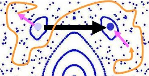
Figure 7: Schematic indicating a direct tunneling process (black arrow) and a chaos-assisted tunneling process (yellow arrow) which would contribute to splitting of bow-tie doublets.

The contribution of chaos-assisted tunneling can be evaluated both qualitatively and quantitatively using the so called “three-level model” ullmo1 ; ullmo2 , where the chaotic energy levels (the eigenstates localized in the chaotic portion of the phase space) are represented by a single state $E_{C}$ with known statistical properties. The straightforward diagonalization of the resulting matrix yields ullmo2

$$\Delta E_{\rm CAT} \simeq \frac{\left|V_{RC}\right|^{2}}{E_{R}-E_{C}}$$ (58)

where $E_{R}$ is the semiclassical energy of the “regular” states (localized at the periodic orbits) which does not include the tunneling contribution, and $V_{RC}$ is the corresponding coupling matrix element with the chaotic state. The resonant denominator in Eq. (58) leads to strong fluctuations of the CAT-related doublets, as is found in numerical simulationsullmo2 . The average behavior of the splittings however is determined by the matrix element $V_{RC}$. By virtue of the Wigner transformation gutz_book it can be shown evgeni1 that $\left|V_{RC}\right|^{2}$ is proportional to the overlap of the Wigner transforms of the ”regular” and “chaotic” states:

$$\left|V_{RC}\right|^{2}\propto\int d\phi\int d\sin\chi\ W_{C}\left(\phi,\sin\chi\right)W_{R}\left(\phi,\sin\chi\right)$$ (59)

Assuming that, as required by Berry’s conjectureberry1 , on the average the Wigner function of a chaotic state is equally distributed across the chaotic portion of the phase space, and using the analytical expressions for the regular eigenstates calculated earlier, we find

$$\langle\Delta E_{\rm CAT}\rangle \propto \exp\left(-{\cal A}kR_{0}\right)$$ (60)

where ${\cal A}$ is the area in the Poincare Surface of Section (in $(\phi,\sin\chi)$ coordinates) occupied by the stable island supporting the regular eigenstate. Note that Eq. (60) holds only on average, since chaos-assisted tunneling always leads to strong fluctuations of the splittings which are of the same order as the average ullmo1 .

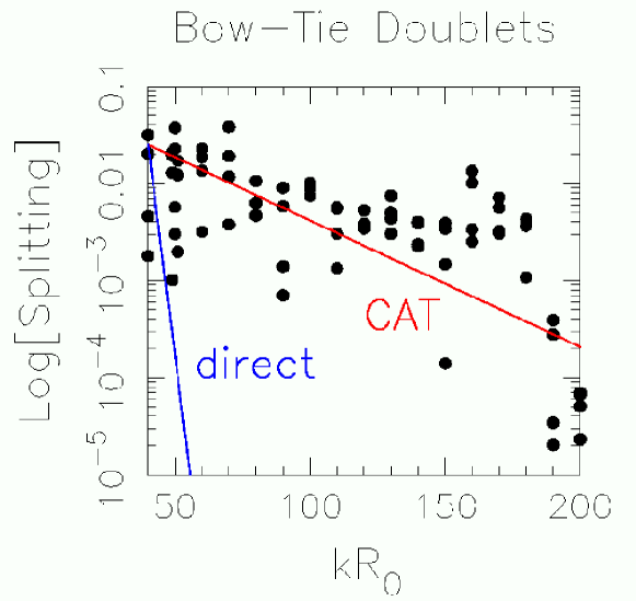
Figure 8: The numerically determined splittings of bow-tie doublets for a closed quadrupole resonator with $\epsilon=0.14$ (black dots) vs kR; the red line denotes the prediction of Eq. (60) for the average splitting, the blue line an estimate of the splitting based on the “direct” coupling. Note the large enhancement due to chaos-assisted tunneling and the large fluctuations around the mean splitting.

In Fig. 8 we show the numerically calculated splittings for the bow-tie resonances in a resonant cavity with a fixed quadrupolar deformation $\epsilon=0.14$, for different values of $kR$. Note that although there are large fluctuations in the numerical data (as previously noted), the data are consistent with Eq. (60), while a calculation based on the “direct” coupling severely underestimates the splittings. Unfortunately, due to the large fluctuations in the splittings, knowledge of the average splitting size does not accurately predict the splitting of a specific doublet. Note also that small violations of symmetry in the fabrication of the resonator may lead to much larger splittings then these tunnel splittings; such an effect was recently observed for triangle-based modes of GaAs ARC micro-lasers gmachl1 .

For the bow-tie orbit the quasi-degeneracy is associated with time-reversal symmetry, but as discussed above, it can equally well be associated with spatial symmetries and indeed this was the situation in the first work on dynamical tunneling DavisHeller . Splittings of this type can also be adequately described using the framework developed in the present section.

V Conclusions

We have generalized gaussian optical resonator theory to describe the resonances associated with stable periodic orbits of arbitrary shaped two-dimensional dielectric resonators using the parabolic equation method. The correspondence to ray optics emerges naturally when imposing the boundary conditions at the dielectric interface which leads to the appropriate ABCD matrices for reflection, transmission and propagation. For a perfectly-reflecting cavity one gets quantized solutions at real values of $k$ localized around the PO with mode spacings given by $\Delta k_{long}=2\pi/L,\Delta k_{trans}=\varphi/L$ where $L$ is the length of the PO and $\varphi$ is the Floquet phase associated with the eigenvalues of the monodromy matrix (round-trip ABCD matrix). For a dielectric cavity one finds similarly localized quasi-bound solutions at quantized complex values of $nk$; in this case the imaginary part of $nk$ is determined by the Fresnel refractive loss at each bounce of the PO. Within this approximation the mode spacings are unchanged from the closed case (except for the trivial factor of $n$). These regular modes coexist in a generic resonator with more complicated modes associated with the chaotic regions of phase space. Generalization of our results to the three-dimensional case appears straightforward for the scalar case and one expects only to have three-dimensional versions of the ABCD matrices enter the theory leading to some difference in details. More interesting would be the inclusion of the polarization degree of freedom, which seems possible in principle, but which we haven’t explored as yet.

We noted that for a cavity with discrete symmetries one will typically be able to construct several symmetry-related, nominally degenerate solutions of the wave equation for each PO. However group-theoretic arguments indicate that the these solutions cannot be exactly degenerate and lead us to construct symmetrized solutions which form quasi-degenerate multiplets. We presented a construction and then two simples rules for calculating the quasi-degeneracy of these multiplets and their symmetry quantum numbers. In the final section of the paper we show that the splittings of these multiplets are much larger than expected, due to the phenomenon of “chaos-assisted” tunneling, and estimate the average splitting in terms of classical quantities.

There are several limitations of this work which we hope to address in future work. One obvious shortcoming is the prediction of zero width modes for the dielectric cavity if the underlying PO has all of its bounces above total internal reflection. Internal reflection is not perfect for these systems at any angle of incidence for two reasons. First, as these solutions describe gaussian beams with some momentum spread, every solution should have some plane-wave amplitude at an angle of incidence for which it can be partially transmitted. This type of correction exists even for a gaussian beam incident on an infinite planar surface and leads to an outgoing beam direction which can be significantly different from that predicted from Snell’s law; we have analyzed the beam deflection for this case recently tureci1 . For the case of the bow-tie modes of the dielectric resonator the effect of the momentum spread in inducing a finite width was also evaluated using a semiclassical method in ref. evgeni2 . Second, due to the curvature of the interface in such resonators, there will always be some evanescent leakage, which we can think of as due to direct tunneling through the angular momentum barrier as is known to occur even for perfectly circular resonators. We have evaluated this type of correction also recently evgeni1 . It is still not clear to what extent these effects can be accounted for systematically within a generalization of our approach here, e.g. to higher order in $kl$. One possibility we are exploring is that a generalized ray optics with non-specular effects included can describe the open resonator and its emission pattern. Both experiments science ; rex1 and numerical studies rex1 ; tureci1 demonstrate that for $kl$ not too large ($\sim 50-100$) these higher order effects must be taken into account.

This work was partially supported by NSF grant DMR-0084501.

References

- (1) R. K. Chang, A. K. Campillo, eds., Optical Processes in Microcavities (World Scientific, Singapore, 1996).
- (2) H. Yokoyama, “Physics and device applications of optical microcavities,” Science 256, 66–70 (1992).
- (3) A. D. Stone, “Wave-chaotic optical resonators and lasers,” Phys. Scr. T90, 248–262 (2001).
- (4) C. Gmachl, F. Capasso, E. E. Narimanov, J. U. Nöckel, A. D. Stone, J. Faist, D. L. Sivco, and A. Y. Cho, “High-power directional emission from microlasers with chaotic resonators,” Science 280, 1556–1564 (1998).
- (5) J. U. Nöckel and A. D. Stone, “Ray and wave chaos in asymmetric resonant optical cavities,” Nature 385, 45–47 (1997).
- (6) A. J. Campillo, J. D. Eversole, and H. B. Lin, “Cavity quantum electrodynamic enhancement of stimulated-emission in microdroplets,” Phys. Rev. Lett. 67, 437–440 (1991).
- (7) H. B. Lin, J. D. Eversole, and A. J. Campillo, “Spectral properties of lasing microdroplets,” J. Opt. Soc. Am. B 9, 43–50 (1992).
- (8) S. M. Spillane, T. J. Kippenberg, and K. J. Vahala, “Ultralow-threshold Raman laser using a spherical dielectric microcavity,” Nature 415, 621–623 (2002).
- (9) B. E. Little, J. S. Foresi, G. Steinmeyer, E. R. Thoen, S. T. Chu, H. A. Haus, E. P. Ippen, L. C. Kimerling, and W. Greene, “Ultra-compact Si-SiO2 microring resonator optical channel dropping filters,” IEEE Photonics Technol. Lett. 10, 549–551 (1998).
- (10) S. X. Qian, J. B. Snow, H. M. Tzeng, and R. K. Chang, “Lasing droplets - highlighting the liquid-air interface by laser-emission,” Science 231, 486–488 (1986).
- (11) A. W. Poon, F. Courvoisier, and R. K. Chang, “Multimode resonances in square-shaped optical microcavities,” Opt. Lett. 26, 632–634 (2001).
- (12) I. Braun, G. Ihlein, F. Laeri, J. U. Nöckel, G. Schulz-Ekloff, F. Schuth, U. Vietze, O. Weiss, and D. Wohrle, “Hexagonal microlasers based on organic dyes in nanoporous crystals,” Appl. Phys. B-Lasers Opt. 70, 335–343 (2000).
- (13) A. Mekis, J. U. Nöckel, G. Chen, A. D. Stone, and R. K. Chang, “Ray chaos and q spoiling in lasing droplets,” Phys. Rev. Lett. 75, 2682–2685 (1995).
- (14) J. U. Nockel, A. D. Stone, G. Chen, H. L. Grossman, and R. K. Chang, “Directional emission from asymmetric resonant cavities,” Opt. Lett. 21, 1609–1611 (1996).
- (15) S. Gianordoli, L. Hvozdara, G. Strasser, W. Schrenk, J. Faist, and E. Gornik, “Long-wavelength quadrupolar-shaped GaAs-AlGaAs microlasers,” IEEE J. Quantum Electron. 36, 458–464 (2000).
- (16) S. Chang, R. K. Chang, A. D. Stone, and J. U. Nöckel, “Observation of emission from chaotic lasing modes in deformed microspheres: displacement by the stable-orbit modes,” J. Opt. Soc. Am. B-Opt. Phys. 17, 1828–1834 (2000).
- (17) N. B. Rex, H. E. Tureci, H. G. L. Schwefel, R. K. Chang, and A. D. Stone, “Fresnel filtering in lasing emission from scarred modes of wave-chaotic optical resonators,” Phys. Rev. Lett. 88, art. no.094 102 (2002).
- (18) N. B. Rex, Regular and chaotic orbit Gallium Nitride microcavity lasers, Ph.D. thesis, Yale University (2001).
- (19) C. Gmachl, E. E. Narimanov, F. Capasso, J. N. Baillargeon, and A. Y. Cho, “Kolmogorov-Arnold-Moser transition and laser action on scar modes in semiconductor diode lasers with deformed resonators,” Opt. Lett. 27, 824–826 (2002).
- (20) S. B. Lee, J. H. Lee, J. S. Chang, H. J. Moon, S. W. Kim, and K. An, “Observation of scarred modes in asymmetrically deformed microcylinder lasers,” Phys. Rev. Lett. 88, art. no.033903 (2002).
- (21) E. J. Heller, “Bound-state eigenfunctions of classically chaotic hamiltonian-systems - Scars of periodic orbits,” Phys. Rev. Lett. 53, 1515–1518 (1984).
- (22) H. G. L. Schwefel, N. B. Rex, H. E. Tureci, R. K. Chang, and A. D. Stone, “Dramatic shape sensitivity of emission patterns for similarly deformed cylindrical polymer lasers,” CLEO/QELS 2002.
- (23) M. V. Berry, “Regularity and chaos in classical mechanics, illustrated by three deformations of a circular billiard,” Eur. J. Phys. 2, 91–102 (1981).
- (24) B. Li and M. Robnik, “Geometry of high-lying eigenfunctions in a plane billiard system having mixed type classical dynamics,” J. Phys. A 28, 2799–2818 (1995).
- (25) J. B. Keller and S. I. Rubinow, “Asymptotic Solution of Eigenvalue Problems,” Ann. Phys. 9, 24–75 (1960).
- (26) M. C. Gutzwiller, Chaos in classical and quantum mechanics (Springer, New York, USA, 1990).
- (27) S. D. Frischat and E. Doron, “Quantum phase-space structures in classically mixed systems: A scattering approach,” J. Phys. A-Math. Gen. 30, 3613–3634 (1997).
- (28) V. M. Babič and V. S. Buldyrev, Asymptotic Methods in Shortwave Diffraction Problems (Springer, New York, USA, 1991).
- (29) A. E. Siegman, Lasers (University Science Books, Mill Valley, California, 1986).
- (30) V. P. Maslov and M. V. Fedoriuk, Semiclassical Approximations in Quantum Mechanics (Reidel, Boston, USA, 1981).
- (31) N. A. Chernikov, “System whose hamiltonian is a time-dependent quadratic form in x and p,” Sov Phys-Jetp Engl Trans 26, 603–608 (1968).
- (32) E. S. C. Ching, P. T. Leung, A. Maassen van den Brink, W. M. Suen, T. S. S., and K. Young, “Quasinormal-mode expansion for waves in open systems,” Rev. Mod. Phys. 70, 1545–1554 (1998).
- (33) J. W. Ra, H. L. Bertoni, and L. B. Felsen, “Reflection and transmission of beams at a dielectric interface,” SIAM J. Appl. Math 24, 396–413 (1973).
- (34) J. M. Robbins, “Discrete symmetries in periodic-orbit theory,” Phys. Rev. A. 40, 2128–2136 (1989).
- (35) M. J. Davis and E. J. Heller, “Multidimensional wave functions from classical trajectories,” J. Chem. Phys. 75, 246 (1981).
- (36) O. Bohigas, S. Tomsovic, and D. Ullmo, “Manifestations of classical phase space structures in quantum mechanics,” Phys. Rep. 223, 45 (1993).
- (37) S. D. Frischat and E. Doron, “Semiclassical description of tunneling in mixed systems: case of the annular billiard,” Phys. Rev. Lett. 75, 3661 (1995).
- (38) F. Leyvraz and D. Ullmo, “The level splitting distribution in chaos-assisted tunneling,” J. Phys. A 29, 2529 (1996).
- (39) E. E. Narimanov, unpublished.
- (40) M. V. Berry, “Regular and irregular semiclassical wavefunctions,” J. Phys. A 10, 2083 (1977).
- (41) H. E. Tureci and A. D. Stone, “Deviation from Snell’s law for beams transmitted near the critical angle: application to microcavity lasers,” Opt. Lett. 27, 7–9 (2002).
- (42) E. E. Narimanov, G. Hackenbroich, P. Jacquod, and A. D. Stone, “Semiclassical theory of the emission properties of wave-chaotic resonant cavities,” Phys. Rev. Lett. 83, 4991–4994 (1999).