Sensitivity Analysis of Stoichiometric Networks: An Extension of Metabolic Control Analysis to Non-equilibrium Trajectories

Abstract

A sensitivity analysis of general stoichiometric networks is considered. The results are presented as a generalization of Metabolic Control Analysis, which has been concerned primarily with system sensitivities at steady state. An expression for time-varying sensitivity coefficients is given, and the Summation and Connectivity Theorems are generalized. The results are compared to previous treatments. The analysis is accompanied by a discussion of the computation of the sensitivity coefficients and an application to a model of phototransduction.

1 Introduction

Sensitivity analysis is an important tool in the study of systems dependent on external parameters. By their nature, stoichiometric networks allow an elegant description of the relationships between component and systemic sensitivities. These relationships, particularly those existing at equilibria of the system, have been addressed by the fields of Biochemical Systems Theory (BST) [17] and Metabolic Control Analysis (MCA) [5, 8].

This paper describes the computation and interpretation of system sensitivities over arbitrary trajectories. The results are presented in the framework provided by MCA, which is a theory devoted to the analysis of the distribution of control within a network and how the behaviour of the system relates to the properties of the components. With few exceptions the MCA literature treats networks in steady state.

MCA has had great success in describing the control and regulation of systems at steady state. However, in the analysis of an increasing domain of examples it becomes necessary to consider sensitivities along non-steady trajectories. In many systems it is the transient or oscillatory behaviour which is of primary interest (e.g. in signal transduction or cell cycle regulation). Some extensions of MCA to non-steady behaviour have appeared in the literature ([1, 4, 7, 11, 12, 15]). These papers generalize the steady state results of MCA to special cases of dynamic behaviour (e.g. periodic behaviour or trajectories near a stable equilibrium). The analysis presented in this paper extends these results by measuring time varying sensitivities along arbitrary trajectories.

A standard MCA analysis might treat, for example, the effect of increasing an enzyme concentration on the steady state value of some related metabolite. Using the analysis described below, one can determine the sensitivity to the perturbation throughout the time evolution of the system, regardless of the nature of the trajectory. Based on these time-varying sensitivities, the Summation and Connectivity Theorems of MCA are extended to give conditions which hold for all time. When applied at steady state, these results reduce to the standard analysis of MCA.

The statements in this paper apply to arbitrary system dynamics, including transients, convergence to steady state, and oscillations. However, as pointed out in previous papers ([4, 11]), sensitivity coefficients derived for oscillating systems must be interpreted with care. A discussion on applications to oscillating systems appears below.

The outline of the paper is as follows. Time-varying sensitivity coefficients are defined and derived, and their computation is discussed briefly. The main results of MCA – the Summation and Connectivity Theorems – are then extended to the time-varying case. Finally, the sensitivity analysis is illustrated by treating some examples, including a model of phototransduction.

2 Preliminaries

A network consisting of $n$ chemical species involved in $m$ reactions is modelled. The $n$-vector ${\bf s}$ is composed of the concentrations of each species. The constant $r$-vector ${\bf p}$ is composed of the (external) parameters of interest in the model. The $m$-vector valued function ${\bf v}={\bf v}({\bf s},{\bf p},t)$ describes the rate of each reaction as a (possibly time-varying) function of species concentrations and parameter values. Finally the $n$ by $m$ stoichiometry matrix ${\bf N}$ describes the network: component ${\bf N}_{i,j}$ is equal to the net number of individuals of species $i$ produced or consumed in reaction $j$. The network can then be modelled by the ordinary differential equation

$$\frac{d}{dt}{\bf s}(t)={\bf N}{\bf v}({\bf s}(t),{\bf p},t)\qquad\hbox{\rm\ for all \ \/}t\geq 0.$$ (1)

We allow the vector ${\bf p}$ to contain the initial states of any of the species concentrations as well as any other parameters which will directly affect the rates of the reactions (e.g. concentrations of enzymes and external effectors).

We assume that the function ${\bf v}({\bf s},{\bf p},t)$ is continuous and is continuously differentiable in ${\bf s}$ and ${\bf p}$ for each fixed $t$. We further assume that for each initial condition ${\bf s}(0)={\bf s}_{0}$ and each choice of parameters ${\bf p}$ the unique solution of (1) is defined for all $t\geq 0$. We denote this solution by ${\bf s}(t,{\bf s}_{0},{\bf p})$, and will use simply ${\bf s}(t,{\bf p})$ or ${\bf s}(t)$ when no confusion will arise.

Before embarking on an analysis of system (1) it is prudent to first consider any linear dependencies inherent in the state variables of the system (which will simplify both the analysis and the computation). Each conserved moiety in the network corresponds to a linearly dependent row in the stoichiometry matrix ${\bf N}$. We follow the procedure and terminology described by Reder [14] (see also [9]) in the reduction of the system.

Let $n_{0}$ denote the row rank of ${\bf N}$. If $n_{0}=n$, then no reduction is necessary. Otherwise, we begin by re-ordering the rows of ${\bf N}$ so that the first $n_{0}$ rows are linearly independent. Let ${\bf N_{R}}$ be the reduced stoichiometry matrix which results from truncating the last $n-n_{0}$ rows of ${\bf N}$. Since the truncated rows can be formed by linear combination of the rows of ${\bf N_{R}}$, the matrix ${\bf N}$ can be written as the product

$${\bf N}={\bf L}{\bf N_{R}}$$

where the $n\times n_{0}$ matrix ${\bf L}$, called the link matrix, has the form

$${\bf L}=\left[\begin{array}[]{c}{\bf I}_{n_{0}}\\ {\bf L_{0}}\end{array}\right].$$

(Here and below the notation ${\bf I}_{q}$ will be used for the $q\times q$ identity matrix).

The advantage of this decomposition can now be realized. Since each conserved moiety allows one species concentration to be determined as a function of the others, we may decompose the species vector ${\bf s}$ into independent and dependent species vectors ${\bf s}_{i}$ and ${\bf s}_{d}$ respectively. Ordering the components of ${\bf s}$ to match the rows of ${\bf N}$, we write ${\bf s}=({\bf s}_{i},{\bf s}_{d})$ where ${\bf s}_{i}$ is an $n_{0}$-tuple and ${\bf s}_{d}$ is an $(n-n_{0})$-tuple. (This involves a minor abuse of notation since ${\bf s}$, ${\bf s}_{i}$ and ${\bf s}_{d}$ are all column vectors.) Then equation (1) can be written as

$$\frac{d}{dt}\left[\begin{array}[]{c}{\bf s}_{i}(t)\\ {\bf s}_{d}(t)\end{array}\right]={\bf L}{\bf N_{R}}{\bf v}({\bf s}(t),{\bf p},t)=\left[\begin{array}[]{c}{\bf I}_{n_{0}}\\ {\bf L_{0}}\end{array}\right]{\bf N_{R}}{\bf v}({\bf s}(t),{\bf p},t)\qquad\hbox{\rm\ for all \ \/}t\geq 0.$$

Hence

$$\frac{d}{dt}{\bf s}_{d}(t)={\bf L_{0}}\frac{d}{dt}{\bf s}_{i}(t)\qquad\hbox{\rm\ for all \ \/}t\geq 0,$$

and so ${\bf s}_{d}(t)-{\bf L_{0}}{\bf s}_{i}(t)$ is an integral of motion of (1), i.e. this difference is constant throughout the evolution of the system. We introduce the constant $(n-n_{0})$-vector ${\bf T}$ to quantify this relationship. Any trajectory of the system satisfies

$${\bf s}_{d}(t)={\bf L_{0}}{\bf s}_{i}(t)+{\bf T}\qquad\hbox{\rm\ for all \ \/}t\geq 0,$$ (4)

where ${\bf T}$ is defined in terms of the initial conditions as

$${\bf T}={\bf s}_{d}(0)-{\bf L_{0}}{\bf s}_{i}(0).$$

In analysis and computation, attention can be restricted to the independent species ${\bf s}_{i}$, since the corresponding results incorporating the dependent vector ${\bf s}_{d}$ are arrived at immediately through the relationship (4). That is, one need only consider the reduced system

$$\frac{d}{dt}{\bf s}_{i}(t)={\bf N_{R}}{\bf v}({\bf s}(t),{\bf p},t)={\bf N_{R}}{\bf v}(({\bf s}_{i}(t),{\bf L_{0}}{\bf s}_{i}(t)+{\bf T}),{\bf p},t)\qquad\hbox{\rm\ for all \ \/}t\geq 0.$$ (5)

3 Sensitivity Analysis

We now present a general sensitivity analysis of the system (1).

3.1 Definitions

Following [18] and [1], we make the basic definition.

Definition 3.1

Given an initial condition ${\bf s}(0)={\bf s}_{0}$ and a set of parameter values ${\bf p}_{0}$, we define the time-varying concentration sensitivity coefficients (or concentration response coefficients) as the elements of the $n\times r$ matrix function ${\bf R^{s}}(\cdot)$ given by

$${\bf R^{s}}(t):=\frac{\partial{\bf s}(t,{\bf p})}{\partial{\bf p}}|_{{\bf p}={\bf p}_{0}}=\lim_{\Delta{\bf p}\rightarrow 0}\frac{{\bf s}(t,{\bf p}_{0}+\Delta{\bf p})-{\bf s}(t,{\bf p}_{0})}{\Delta{\bf p}}\qquad\hbox{\rm\ for all \ \/}t\geq 0.$$

$\Box$

Remark 3.2

These time varying response coefficients can be interpreted in exact analogy to the standard (steady state) response coefficients of MCA. The difference is that the response to a perturbation along an entire trajectory in now considered, rather than at a particular equilibrium state.

Take for example a system which has an asymptotically stable equilibrium (say ${\bf s}^{ss}$), and consider a set of initial conditions (say ${\bf s}_{0}$) which do not match the steady state solution. Letting the system evolve from ${\bf s}_{0}$, we may observe some initial transient, followed by convergence to ${\bf s}^{ss}$ as time tends to infinity. Alternatively, if we make a small perturbation to a system parameter, we may observe a different transient, followed by convergence to a different steady state. The response coefficient defined above provides a measure of the difference between this “perturbed trajectory” and the “nominal” (unperturbed) trajectory at each time $t$. As time tends to infinity, each trajectory will converge to its steady state, and so the response coefficient will converge to the steady state response of MCA.

This time-history analysis is particularly useful when studying systems in which transient behaviour plays a key role in the mechanism. For example, in systems performing phototransduction or action potential transfer, the role of the system is to produce a (transient) spike in the concentration of a certain species. The analysis presented here will allow elucidation of the effect of parameter perturbations on the behaviour of such a system.

It should be noted that the response coefficient ${\bf R^{s}}(\cdot)$ is defined with respect to a particular parameter choice ${\bf p}_{0}$ and a particular initial condition ${\bf s}_{0}$. Should one be interested in comparing the system response to perturbations at different times, a separate response coefficient must be defined for each such time, since each choice will yield a distinct “initial” state (by re-setting time to zero at the point chosen). $\Box$

Remark 3.3

Since the vector ${\bf p}$ is allowed to contain the initial states as components, sensitivity coefficients with respect to initial conditions are included in the above definition. When pursuing a steady state analysis, it is often more convenient to consider the total amount of each conserved moiety as a parameter rather than the initial conditions of particular species (see e.g. [9]). However, in this dynamic analysis, perturbation of the initial concentrations of different species will have distinct effects on the time-history; it is only at steady state that these effects can be described equivalently in terms of perturbations in pools of conserved moieties. $\Box$

In addition to the sensitivities of the species concentrations, it is also of interest to consider the sensitivities of the various rates ${\bf v}({\bf s},{\bf p},t)$. In expressing these responses, we conform to the MCA usage of the term flux for the rate of a system reaction. (In general, these rates do not represent fluxes in the usual sense of the word as a rate of transfer of some quantity; the rate of passage of mass through a reaction pathway must also take the stoichiometry into consideration.)

Definition 3.4

Given an initial condition ${\bf s}(0)={\bf s}_{0}$ and set of parameter values ${\bf p}_{0}$, we define the time-varying flux sensitivity coefficients (or flux response coefficients) as the elements of the $m\times r$ matrix function ${\bf R^{J}}(\cdot)$ given by

$${\bf R^{J}}(t):=\frac{\partial{\bf v}({\bf s}(t,{\bf p}),{\bf p},t)}{\partial{\bf p}}|_{{\bf p}={\bf p}_{0}} = \frac{\partial{\bf v}({\bf s},{\bf p},t)}{\partial{\bf s}}\frac{\partial{\bf s}(t,{\bf p})}{\partial{\bf p}}+\frac{\partial{\bf v}({\bf s},{\bf p},t)}{\partial{\bf p}}$$

$$= \frac{\partial{\bf v}({\bf s},{\bf p},t)}{\partial{\bf s}}{\bf R^{s}}(t)+\frac{\partial{\bf v}({\bf s},{\bf p},t)}{\partial{\bf p}}\qquad\hbox{\rm\ for all \ \/}t\geq 0,$$

where the derivatives are evaluated at ${\bf p}={\bf p}_{0}$ and ${\bf s}={\bf s}(t,{\bf p}_{0})$. $\Box$

Remark 3.5

The flux response coefficients can be interpreted analogously to the concentration response coefficients: ${\bf R^{J}}(t)$ gives the response in the rates at time $t$ to a perturbation at time zero. At steady state, these coefficients reduce to their standard MCA counterparts. $\Box$

3.2 Computation

The sensitivity coefficients are defined by a first-order linear ordinary differential equation which follows from taking the derivative of (1) with respect to ${\bf p}$. Dropping some functional dependencies for ease of legibility, we have:

$$\frac{\partial}{\partial{\bf p}}\frac{d{\bf s}(t)}{dt}={\bf N}\left(\frac{\partial{\bf v}(t)}{\partial{\bf s}}\frac{\partial{\bf s}(t)}{\partial{\bf p}}+\frac{\partial{\bf v}(t)}{\partial{\bf p}}\right)\qquad\hbox{\rm\ for all \ \/}t\geq 0$$

which becomes, after switching the order of differentiation,

$$\frac{d}{dt}\frac{\partial{\bf s}(t)}{\partial{\bf p}}={\bf N}\left(\frac{\partial{\bf v}(t)}{\partial{\bf s}}\frac{\partial{\bf s}(t)}{\partial{\bf p}}+\frac{\partial{\bf v}(t)}{\partial{\bf p}}\right)\qquad\hbox{\rm\ for all \ \/}t\geq 0.$$ (6)

Recall that the sensitivity coefficients are defined with respect to a particular choice of ${\bf s}_{0}={\bf s}(0)$ and ${\bf p}_{0}$. This choice fixes a trajectory ${\bf s}(t)={\bf s}(t,{\bf s}_{0},{\bf p}_{0})$, and hence determines the function ${\bf v}(t)={\bf v}({\bf s}(t),{\bf p},t)$ as well. The initial conditions for (6) (i.e. the components of the matrix $\frac{\partial{\bf s}}{\partial{\bf p}}(0)$) are immediate from the definition of the sensitivity coefficients: the $j,k$-th entry of $\frac{\partial{\bf s}}{\partial{\bf p}}(0)$ will be zero unless the $k$-th parameter is the initial condition of the $j$-th species, in which case the initial value of the sensitivity coefficient will be one. Equation (6) can be solved for the concentration sensitivities $\frac{\partial{\bf s}}{\partial{\bf p}}(\cdot)={\bf R^{s}}(\cdot)$, and the flux sensitivities can be computed according to definition 3.4. However, we can reduce the burden of computation by taking advantage of the dependencies described in equation (4).

Differentiating (5) with respect to ${\bf p}$, we find

$$\frac{\partial}{\partial t}\frac{\partial{\bf s}_{i}(t)}{\partial{\bf p}} = {\bf N_{R}}\left(\frac{\partial{\bf v}(t)}{\partial{\bf s}_{i}}\frac{\partial{\bf s}_{i}(t)}{\partial{\bf p}}+\frac{\partial{\bf v}(t)}{\partial{\bf s}_{d}}\frac{\partial}{\partial{\bf p}}({\bf L_{0}}{\bf s}_{i}(t)+{\bf T})+\frac{\partial{\bf v}(t)}{\partial{\bf p}}\right)$$ (7)

$$= {\bf N_{R}}\left[\left(\frac{\partial{\bf v}(t)}{\partial{\bf s}_{i}}+\frac{\partial{\bf v}(t)}{\partial{\bf s}_{d}}{\bf L_{0}}\right)\frac{\partial{\bf s}_{i}(t)}{\partial{\bf p}}+\frac{\partial{\bf v}(t)}{\partial{\bf s}_{d}}\frac{\partial{\bf T}}{\partial{\bf p}}+\frac{\partial{\bf v}(t)}{\partial{\bf p}}\right]$$

$$= {\bf N_{R}}\left[\frac{\partial{\bf v}(t)}{\partial{\bf s}}{\bf L}\frac{\partial{\bf s}_{i}(t)}{\partial{\bf p}}+\frac{\partial{\bf v}(t)}{\partial{\bf s}_{d}}\frac{\partial{\bf T}}{\partial{\bf p}}+\frac{\partial{\bf v}(t)}{\partial{\bf p}}\right]\qquad\hbox{\rm\ for all \ \/}t\geq 0.$$

The initial conditions are determined as before.

Remark 3.6

While there are special cases in which the response coefficients can be derived explicitly (as discussed below), in most cases the solution to equation (6) (or more efficiently (7)) must be computed numerically. In performing such a calculation, one must keep in mind that the right-hand-side depends on the time-varying value of the species concentration vector ${\bf s}(t)$. A simple computational strategy is to solve (5) and (7) as a single set of differential equations, determining ${\bf s}_{i}(\cdot)$ and $\frac{\partial{\bf s}_{i}(\cdot)}{\partial{\bf p}}$ simultaneously. This would allow, for example, an adaptive integrator to reduce the step-size during computation should either equation demand it.

The reader should note that the pair of ODE’s are coupled, but that the coupling is in cascade – equation (5) is independent of $\frac{\partial{\bf s}_{i}(\cdot)}{\partial{\bf p}}$. Thus the increase in complexity comes simply from having two equations to solve, not from any intertwining of the solutions.

An algorithm for computation of the time-varying response coefficients has been implemented in MATLAB and in the biochemical simulator Jarnac [16]. Scripts of the implementation are available online (http://www.sys-bio.org). $\Box$

3.3 Analytical Solution

The solution to equation (7) can be expressed in terms of the variation of parameters formula (derived in standard texts on ODE’s, e.g. [3]):

$$\frac{\partial{\bf s}_{i}}{\partial{\bf p}}(t)=\Phi(t)\frac{\partial{\bf s}_{i}}{\partial{\bf p}}(0)+\Phi(t)\int_{0}^{t}\Phi^{-1}(\tau){\bf N_{R}}\left(\frac{\partial{\bf v}(\tau)}{\partial{\bf s}_{d}}\frac{\partial{\bf T}}{\partial{\bf p}}+\frac{\partial{\bf v}(\tau)}{\partial{\bf p}}\right)\,d\tau\qquad\hbox{\rm\ for all \ \/}t\geq 0,$$ (8)

where the matrix-valued function $\Phi(\cdot)$ (called the fundamental matrix for equation (7)) satisfies the homogeneous part of (7), i.e. $\Phi(\cdot)$ is defined as the solution of the following initial value problem

$$\frac{d}{dt}\Phi(t)=\left[{\bf N_{R}}\frac{\partial{\bf v}(t)}{\partial{\bf s}}{\bf L}\right]\Phi(t),\qquad\Phi(0)={\bf I}_{n_{0}}.$$ (9)

Note that (8) does not in general provide an explicit formula for the solution to (7) (since (9) does not admit an explicit solution, in general). Nevertheless, knowing the solution takes this form can simplify both analysis and computation. In addition, as will be demonstrated in Section 4, there are special cases in which (8) does indeed provide an explicit solution.

In the subsequent analysis, it will be convenient to partition the parameter vector ${\bf p}$ into the set of parameters which affect the rates (denoted ${\bf p}_{v}$) and the set of initial conditions (denoted ${\bf p}_{s}$). From the fact that $\frac{\partial{\bf v}}{\partial{\bf p}_{s}}=\frac{\partial{\bf s}_{i}}{\partial{\bf p}_{v}}(0)=\frac{\partial{\bf T}}{\partial{\bf p}_{v}}=0$, we see that formula (8) can be partitioned as

$$\frac{\partial{\bf s}_{i}}{\partial{\bf p}_{s}}(t) = \Phi(t)\frac{\partial{\bf s}_{i}}{\partial{\bf p}_{s}}(0)+\Phi(t)\int_{0}^{t}\Phi^{-1}(\tau){\bf N_{R}}\frac{\partial{\bf v}(\tau)}{\partial{\bf s}_{d}}\frac{\partial{\bf T}}{\partial{\bf p}_{s}}\,d\tau$$

$$\frac{\partial{\bf s}_{i}}{\partial{\bf p}_{v}}(t) = \Phi(t)\int_{0}^{t}\Phi^{-1}(\tau){\bf N_{R}}\frac{\partial{\bf v}(\tau)}{\partial{\bf p}_{v}}\,d\tau\qquad\hbox{\rm\ for all \ \/}t\geq 0.$$ (10)

To provide a more elegant exposition in what follows, we consider the extension of (10) to the entire response coefficient matrix ${\bf R^{s}}(\cdot)=\frac{\partial{\bf s}}{\partial{\bf p}}(\cdot)$. Since ${\bf s}_{d}(t)={\bf L_{0}}{\bf s}_{i}(t)+{\bf T}$ for all $t\geq 0$ and $\frac{\partial{\bf T}}{\partial{\bf p}_{v}}=0$, (10) gives

$$\frac{\partial{\bf s}_{d}}{\partial{\bf p}_{v}}(t)={\bf L_{0}}\Phi(t)\int_{0}^{t}\Phi^{-1}(\tau){\bf N_{R}}\frac{\partial{\bf v}(\tau)}{\partial{\bf p}_{v}}\,d\tau\qquad\hbox{\rm\ for all \ \/}t\geq 0.$$ (11)

Together, (10) and (11) give

$$\frac{\partial{\bf s}}{\partial{\bf p}_{v}}(t)={\bf L}\Phi(t)\int_{0}^{t}\Phi^{-1}(\tau){\bf N_{R}}\,\frac{\partial{\bf v}(\tau)}{\partial{\bf p}_{v}}d\tau\qquad\hbox{\rm\ for all \ \/}t\geq 0.$$ (12)

As for the flux-response coefficients,

$$\frac{\partial{\bf v}}{\partial{\bf p}_{v}}(t)=\frac{\partial{\bf v}(t)}{\partial{\bf s}}{\bf L}\Phi(t)\int_{0}^{t}\Phi^{-1}(\tau){\bf N_{R}}\frac{\partial{\bf v}(\tau)}{\partial{\bf p}_{v}}\,d\tau+\frac{\partial{\bf v}(t)}{\partial{\bf p}_{v}}\qquad\hbox{\rm\ for all \ \/}t\geq 0.$$

3.4 Scaled Coefficients

Computations in MCA are typically done using “scaled” coefficients: derivatives are taken with respect to the logarithms of the variables, giving relative (rather than absolute) responses. These scaled sensitivities have the advantage that they are dimensionless. Further, they allow direct comparison of responses at different states or across different parameters.

The scaled responses are related to their unscaled counterparts through multiplication by a ratio of the values involved. These relationships can be elegantly described at the matrix level. Following [9], we define the diagonal matrices

$${\bf D^{s}}(\cdot):=\hbox{\rm\ diag\ \/}{\bf s}(\cdot)\qquad{\bf D^{v}}(\cdot):=\hbox{\rm\ diag\ \/}{\bf v}({\bf s}(\cdot),{\bf p},\cdot)\qquad{\bf D^{p}}:=\hbox{\rm\ diag\ \/}{\bf p}$$

whose entries are given by the coefficients of the corresponding vectors. The scaled response matrices, denoted with a “tilde” ($\widetilde{\phantom{a}}$) are then given by

$$\bf{\widetilde{R}^{s}}(\cdot) = ({\bf D^{s}}(\cdot))^{-1}{\bf D^{p}}{\bf R^{s}}(\cdot)=\frac{\partial\ln{\bf s}(\cdot)}{\partial\ln{\bf p}}$$

$$\bf{\widetilde{R}^{v}}(\cdot) = ({\bf D^{v}}(\cdot))^{-1}{\bf D^{p}}{\bf R^{J}}(\cdot)=\frac{\partial\ln{\bf v}(\cdot)}{\partial\ln{\bf p}}.$$

4 MCA Theorems

We next consider generalizations of the main results of Metabolic Control Analysis to the case of time-varying sensitivities. These results (the Summation and Connectivity Theorems, and the resulting Control-Matrix Equation) are usually stated in terms of control coefficients and elasticities, into which the response coefficient matrices are factored ([14, 9]). The time varying responses defined above do not, in general, allow such a factorization. However, the responses can be interpreted as the result of applying an appropriately defined control operator to an elasticity. In this sense, the standard MCA results can be extended to the time-varying case. Moreover, we will show that under certain assumptions on the derivatives of the rates, one can recover direct generalizations in terms of matrix factorizations (as was done in [7]).

4.1 Control Operators

Given a trajectory of system (1), we define the substrate- and parameter-elasticities of the system as

$${\bf\varepsilon}_{{\bf s}}(t):=\frac{\partial{\bf v}}{\partial{\bf s}}(t)\qquad{\bf\varepsilon}_{{\bf p}}(t):=\frac{\partial{\bf v}}{\partial{\bf p}}(t)\qquad\hbox{\rm\ for all \ \/}t\geq 0.$$

These vectors describe component (or “local”) sensitivities of the isolated reactions associated with the system.

The steady state Summation and Connectivity Theorems admit elegant mathematical descriptions due to the fact that the steady state concentration and flux responses can each be decomposed into a product of two terms: a matrix of control coefficients and a vector of parameter elasticities. It is clear from equation (12) that the general time-varying response cannot be expressed as a product involving the parameter elasticities (since this time-varying term appears inside the integral). However, the relation between response and elasticity can be expressed as the action of a control operator on the elasticity vector, as follows. (An operator, in this case, is an object that maps functions to functions. An introduction to operators appears in the appendix.)

Definition 4.1

The concentration control operator ${\bf C^{s}}$ maps $m$-vector valued functions to $n$-vector valued functions as follows. Given a continuous $m$-vector valued function $y(\cdot)$ defined on the non-negative reals, ${\bf C^{s}}(\cdot)(y(\cdot))$ is an $n$-vector valued function defined by

$${\bf C^{s}}(t)(y(\cdot)):={\bf L}\Phi(t)\int_{0}^{t}\Phi^{-1}(\tau){\bf N_{R}}\,y(\tau)\,d\tau\qquad\hbox{\rm\ for all \ \/}t\geq 0.$$

$\Box$

In a like manner we define the flux control operator.

Definition 4.2

The flux control operator ${\bf C^{J}}$ maps $m$-vector valued functions to $m$-vector valued functions as follows. Given a continuous $m$-vector valued function $y(\cdot)$ defined on the non-negative reals, ${\bf C^{J}}(\cdot)(y(\cdot))$ is an $m$-vector valued function defined by

$${\bf C^{J}}(t)(y(\cdot)):={\bf\varepsilon}_{{\bf s}}(t){\bf C^{s}}(t)(y(\cdot))+y(t)\qquad\hbox{\rm\ for all \ \/}t\geq 0.$$

$\Box$

The elasticities and control operators can be scaled in the same manner as the response coefficients. Each of the results described below has an analogous statement in terms of scaled quantities, determined simply by including the scaling factors.

With these definitions in hand, the generalizations of the partitioned response properties ([10, 9]) follow immediately. If the parameter vector is such that the parameters only affect the rates (i.e. ${\bf p}={\bf p}_{v}$), then

$${\bf R^{s}}(t)={\bf C^{s}}(t)({\bf\varepsilon}_{\bf p}(\cdot))\qquad{\bf R^{J}}(t)={\bf C^{J}}(t)({\bf\varepsilon}_{\bf p}(\cdot))\qquad\hbox{\rm\ for all \ \/}t\geq 0.$$

We next indicate how the Summation and Connectivity Theorems can be interpreted in the light of these definitions. We will also show how the action of these operators reduces to matrix multiplication when the system is at steady state.

4.2 The Summation Theorem

The Summation Theorem can be stated in terms of the control operators as follows.

Theorem 1

(Summation Theorem) If the $m$-vector ${\bf k}$ lies in the nullspace of ${\bf N}$ (i.e. ${\bf N}{\bf k}=0$, and so ${\bf N_{R}}{\bf k}=0$ as well), then (using the simplified notation described in the appendix)

$${\bf C^{s}}(t)({\bf k})=0\qquad\hbox{\rm\ and\ \/}\qquad{\bf C^{J}}(t)({\bf k})={\bf k}\qquad\hbox{\rm\ for all \ \/}t\geq 0.$$

Proof. The result follows from the definitions of the control operators. If ${\bf N_{R}}{\bf k}=0$, then

$${\bf C^{s}}(t)({\bf k})={\bf L}\Phi(t)\int_{0}^{t}\Phi^{-1}(\tau){\bf N_{R}}\,{\bf k}\,d\tau=0\qquad\hbox{\rm\ for all \ \/}t\geq 0,$$

and

$${\bf C^{J}}(t)({\bf k})=\varepsilon_{\bf s}{\bf C^{s}}(t)({\bf k})+{\bf k}={\bf k}\qquad\hbox{\rm\ for all \ \/}t\geq 0.$$

 

To state the result in a more standard form, we allow the control operators to act on matrices as follows. If ${\bf r}_{1}(\cdot),\ldots,{\bf r}_{n}(\cdot)$ are $m$-vector valued functions, then we interpret

$${\bf C^{s}}(t)([{\bf r}_{1}(\cdot)\ldots{\bf r}_{n}(\cdot)]):=\left[{\bf C^{s}}(t)({\bf r}_{1}(\cdot))\ldots{\bf C^{s}}(t)({\bf r}_{n}(\cdot))\right].$$

With this notation, a direct corollary of the Summation Theorem is the following.

Corollary 4.3

If the matrix ${\bf K}$ has columns which form a basis for the nullspace of ${\bf N}$, then

$${\bf C^{s}}(t)({\bf K})=0\qquad\hbox{\rm\ and\ \/}\qquad{\bf C^{J}}(t)({\bf K})={\bf K}\qquad\hbox{\rm\ for all \ \/}t\geq 0.$$

 

The Summation Theorem is normally stated as a property of the control coefficients of a system at steady state. However, the steady state version can be given an equivalent formulation which does not make reference to control coefficients.

Proposition 4.4

(Summation Theorem – steady state) Suppose the system is at steady state, so we may drop time dependencies on all terms. If the parameter vector is such that the parameters only affect the rates (i.e. ${\bf p}={\bf p}_{v}$) and each column of the matrix ${\bf\varepsilon_{p}}=\frac{\partial{\bf v}}{\partial{\bf p}}$ lies in the nullspace of ${\bf N}$, then

$${\bf R^{s}}=0\qquad\hbox{\rm\ and\ \/}\qquad{\bf R^{J}}={\bf\varepsilon_{p}}.$$

 

Stated in this way, the Theorem can be extended directly to time-varying responses. From Theorem 1, we have the following.

Corollary 4.5

(Summation Theorem – alternative statement) If the parameter vector is such that the parameters only affect the rates (i.e. ${\bf p}={\bf p}_{v}$) and each column of the matrix ${\bf\varepsilon_{p}}(t)=\frac{\partial{\bf v}}{\partial{\bf p}}(t)$ lies in the nullspace of ${\bf N_{R}}$ for each $t\geq 0$, then

$${\bf R^{s}}(t)=0\qquad\hbox{\rm\ and\ \/}\qquad{\bf R^{J}}(t)={\bf\varepsilon_{p}}(t)\qquad\hbox{\rm\ for all \ \/}t\geq 0.$$

 

4.2.1 Special Case: ${\bf\varepsilon_{p}}$ constant

In special cases, Theorem 1 reduces to more familiar variants. A simplification which can be made to the general case described above is to assume that some derivatives of the rate law ${\bf v}(\cdot,\cdot,\cdot)$ are constant throughout the evolution of the system. This was the case considered by Heinrich and Reder in [7], where it was argued that for systems near a stable equilibrium, it may be reasonable to approximate the derivatives of ${\bf v}$ by their values at the equilibrium.

If one restricts to the special case where the parameter elasticity ${\bf\varepsilon_{p}}$ is constant throughout the evolution of the system, the control operators need not be defined to act on arbitrary functions, but only on constant $m$-vectors. The action of the operators can in this case be described simply as matrix multiplication, e.g. for any constant $m$-vector ${\bf y}$,

$${\bf C^{s}}(t)({\bf y})=\left[{\bf L}\Phi(t)\int_{0}^{t}\Phi^{-1}(\tau){\bf N_{R}}\,d\tau\,\right]{\bf y}\qquad\hbox{\rm\ for all \ \/}t\geq 0.$$

In this case, through a slight abuse of notation, time varying control coefficients can be defined by

$${\bf C^{s}}(t) := {\bf L}\Phi(t)\int_{0}^{t}\Phi^{-1}(\tau){\bf N_{R}}\,d\tau$$

$${\bf C^{J}}(t) := \varepsilon_{{\bf s}}(t){\bf L}\Phi(t)\int_{0}^{t}\Phi^{-1}(\tau){\bf N_{R}}\,d\tau+{\bf I}_{m}$$

Here, we can state a more standard Summation Theorem: if the matrix ${\bf K}$ has columns which form a basis for the null space of ${\bf N}$ (equivalently of ${\bf N_{R}}$), then for all $t\geq 0$,

$${\bf C^{s}}(t){\bf K} = 0$$

$${\bf C^{J}}(t){\bf K} = {\bf K},$$

where the left-hand-side is interpreted as a matrix product.

4.3 Connectivity Theorem

The Connectivity Theorem for control operators is as follows.

Theorem 2

(Connectivity Theorem) Applying the control operators to the function ${\bf\varepsilon}_{\bf s}(\cdot){\bf L}=\frac{\partial{\bf v}}{\partial{\bf s}}(\cdot){\bf L}$ yields, for all $t\geq 0$,

$${\bf C^{s}}(t)({\bf\varepsilon}_{\bf s}(\cdot){\bf L}) = {\bf L}(\Phi(t)-{\bf I}_{n_{0}})$$

$${\bf C^{J}}(t)({\bf\varepsilon}_{\bf s}(\cdot){\bf L}) = {\bf\varepsilon}_{\bf s}(t){\bf L}\Phi(t).$$

While the right-hand-sides of the equations above may not look familiar, the reader should note that if $\Phi(t)=0$ then these reduce to more standard connectivity relations. In what follows we will consider a case where $\Phi(t)$ approaches zero as steady state is reached, so that the classical MCA result is recovered.

Proof. The definition of the concentration control operator gives

$${\bf C^{s}}(t)(\frac{\partial{\bf v}}{\partial{\bf s}}(\cdot){\bf L})={\bf L}\Phi(t)\int_{0}^{t}\Phi^{-1}(\tau){\bf N_{R}}\,\frac{\partial{\bf v}(\tau)}{\partial{\bf s}}{\bf L}\,d\tau\qquad\hbox{\rm\ for all\ \/}t\geq 0.$$ (13)

From equation (9), we have that

$$\left[\frac{d}{dt}\Phi(t)\right]\Phi^{-1}(t)={\bf N_{R}}\frac{\partial{\bf v}(t)}{\partial{\bf s}}{\bf L}\qquad\hbox{\rm\ for all \ \/}t\geq 0.$$ (14)

Moreover, from the fact that

$$0=\frac{d}{dt}{\bf I}_{n_{0}}=\frac{d}{dt}[\Phi(t)\Phi^{-1}(t)]=\left[\frac{d}{dt}\Phi(t)\right]\Phi^{-1}(t)+\Phi(t)\left[\frac{d}{dt}\Phi^{-1}(t)\right],$$

we see that

$$\frac{d}{dt}\Phi^{-1}(t)=-\Phi^{-1}(t)\left[\frac{d}{dt}\Phi(t)\right]\Phi^{-1}(t)\qquad\hbox{\rm\ for all \ \/}t\geq 0.$$

Thus, from (13) and (14),

$${\bf C^{s}}(t)(\frac{\partial{\bf v}}{\partial{\bf s}}(\cdot){\bf L}) = {\bf L}\Phi(t)\int_{0}^{t}\Phi^{-1}(\tau){\bf N_{R}}\,\frac{\partial{\bf v}(\tau)}{\partial{\bf s}}{\bf L}\,d\tau$$

$$= {\bf L}\Phi(t)\int_{0}^{t}\Phi^{-1}(\tau)\left[\frac{d}{d\tau}\Phi(\tau)\right]\Phi^{-1}(\tau)\,d\tau$$

$$= -{\bf L}\Phi(t)\int_{0}^{t}\frac{d}{d\tau}\Phi^{-1}(\tau)\,d\tau\qquad\hbox{\rm\ for all \ \/}t\geq 0.$$

Application of the Fundamental Theorem of Calculus gives

$${\bf C^{s}}(t)(\frac{\partial{\bf v}}{\partial{\bf s}}(\cdot){\bf L}) = -{\bf L}\Phi(t)[\Phi^{-1}(t)-\Phi^{-1}(0)]$$

$$= {\bf L}(\Phi(t)-{\bf I}_{n_{0}})\qquad\hbox{\rm\ for all \ \/}t\geq 0,$$

as $\Phi^{-1}(0)={\bf I}_{n_{0}}=\Phi(0)$. With the definition of the flux control operator, we conclude

$${\bf C^{J}}(t)(\varepsilon_{{\bf s}}(\cdot){\bf L}) = \varepsilon_{{\bf s}}(t){\bf L}(\Phi(t)-{\bf I}_{n_{0}})+\varepsilon_{{\bf s}}(t){\bf L}$$

$$= \varepsilon_{{\bf s}}(t){\bf L}\Phi(t)\qquad\hbox{\rm\ for all \ \/}t\geq 0.$$

 

The Connectivity Theorem is typically stated as a property of the steady state control coefficients. As is the case for the Summation Theorem, an equivalent formulation can be given which does not make reference to control coefficients, as follows.

Proposition 4.6

(Connectivity Theorem – steady state) Suppose the system is at steady state, so we may drop time dependencies on all terms. If the parameter vector is such that the parameters only affect the rates (i.e. ${\bf p}={\bf p}_{v}$) and the elasticities satisfy $\varepsilon_{{\bf p}}={\bf\varepsilon}_{\bf s}{\bf L}$, then

$${\bf R^{s}}=-{\bf L}\qquad\hbox{\rm\ and\ \/}\qquad{\bf R^{J}}=0.$$

 

There is a direct extension to the general case. From Theorem 2, we have the following.

Corollary 4.7

(Connectivity Theorem – alternative statement) If the parameter vector is such that the parameters only affect the rates (i.e. ${\bf p}={\bf p}_{v}$) and the elasticities satisfy $\varepsilon_{{\bf p}}(t)={\bf\varepsilon}_{\bf s}(t){\bf L}$ for each $t\geq 0$, then

$${\bf R^{s}}(t)={\bf L}(\Phi(t)-{\bf I}_{n_{0}})\qquad\hbox{\rm\ and\ \/}\qquad{\bf R^{J}}(t)={\bf\varepsilon}_{\bf s}(t){\bf L}\Phi(t)\qquad\hbox{\rm\ for all \ \/}t\geq 0.$$

 

4.3.1 Special Case: $\varepsilon_{{\bf s}}$ and $\varepsilon_{{\bf p}}$ constant

Again, in the special case where the derivatives of ${\bf v}(\cdot,\cdot,\cdot)$ are constant throughout the trajectory, the analysis simplifies.

If $\varepsilon_{{\bf s}}=\frac{\partial{\bf v}}{\partial{\bf s}}$ is constant throughout the evolution of the system, the fundamental matrix defined by equation (9) can be described explicitly as the matrix exponential

$$\Phi(t)=e^{{\bf N_{R}}\varepsilon_{{\bf s}}{\bf L}t}\qquad\hbox{\rm\ for all \ \/}t\geq 0.$$

In this case (8) provides an explicit formula for the sensitivity coefficients.

Heinrich and Reder considered the case in which both $\varepsilon_{{\bf p}}$ and $\varepsilon_{{\bf s}}$ are constant along the trajectory of the system in [7]. In that case, the control operators again need only be defined on constant vectors, their action reducing to matrix multiplication. That is, given any constant $m$-vector ${\bf y}$,

$${\bf C^{s}}(t)({\bf y}) = \left[{\bf L}e^{{\bf N_{R}}\varepsilon_{{\bf s}}{\bf L}t}\int_{0}^{t}e^{-{\bf N_{R}}\varepsilon_{{\bf s}}{\bf L}\tau}{\bf N_{R}}\,d\tau\right]{\bf y}$$ (15)

$$= \left[{\bf L}\int_{0}^{t}e^{{\bf N_{R}}\varepsilon_{{\bf s}}{\bf L}(t-\tau)}{\bf N_{R}}\,d\tau\right]{\bf y}\qquad\hbox{\rm\ for all \ \/}t\geq 0.$$

The matrix ${\bf N_{R}}\varepsilon_{{\bf s}}{\bf L}$ is the Jacobian of equation (5). In the case where it is nonsingular, (15) further reduces to

$${\bf C^{s}}(t)({\bf y}) = \left[{\bf L}(e^{{\bf N_{R}}\varepsilon_{{\bf s}}{\bf L}t}-{\bf I}_{n_{0}})({\bf N_{R}}\varepsilon_{{\bf s}}{\bf L})^{-1}{\bf N_{R}}\right]{\bf y}\qquad\hbox{\rm\ for all \ \/}t\geq 0.$$

This assumption of nonsingularity is rather standard (see, e.g. [14]); in particular, it holds when the analysis is being carried out near an asymptotically stable equilibrium point.

Under these assumptions the control coefficients take the form of the time-varying matrices

$${\bf C^{s}}(t) := {\bf L}(e^{{\bf N_{R}}\varepsilon_{{\bf s}}{\bf L}t}-{\bf I}_{n_{0}})({\bf N_{R}}\varepsilon_{{\bf s}}{\bf L})^{-1}{\bf N_{R}}$$

$${\bf C^{J}}(t) := \varepsilon_{{\bf s}}{\bf L}(e^{{\bf N_{R}}\varepsilon_{{\bf s}}{\bf L}t}-{\bf I}_{n_{0}})({\bf N_{R}}\varepsilon_{{\bf s}}{\bf L})^{-1}{\bf N_{R}}+{\bf I}_{m},$$

and the Connectivity Theorem reduces to the form presented in [7]: for all $t\geq 0$,

$${\bf C^{s}}(t){\bf\varepsilon}_{\bf s}{\bf L} = {\bf L}(e^{{\bf N_{R}}{\bf\varepsilon}_{\bf s}{\bf L}t}-{\bf I}_{n_{0}})$$

$${\bf C^{J}}(t){\bf\varepsilon}_{\bf s}{\bf L} = {\bf\varepsilon}_{\bf s}{\bf L}e^{{\bf N_{R}}{\bf\varepsilon}_{\bf s}{\bf L}t}.$$

If such a a trajectory further satisfies the condition that it is approaching an asymptotically stable steady state, then it will be the case that

$$\lim_{t\rightarrow\infty}e^{{\bf N_{R}}{\bf\varepsilon}_{\bf s}{\bf L}t}=0.$$

Then, taking limits, we find that the control coefficients reduce to their standard forms [14] as the steady state is approached,

$$\lim_{t\rightarrow\infty}{\bf C^{s}}(t) = -{\bf L}({\bf N_{R}}{\bf\varepsilon}_{\bf s}{\bf L})^{-1}{\bf N_{R}}$$

$$\lim_{t\rightarrow\infty}{\bf C^{J}}(t) = -{\bf\varepsilon}_{\bf s}{\bf L}({\bf N_{R}}{\bf\varepsilon}_{\bf s}{\bf L})^{-1}{\bf N_{R}}+{\bf I}_{m}.$$

The time-varying Summation and Connectivity Theorems described above reduce to the standard statements in this case, as described in [7].

4.4 Control Matrix Equation

Together, the steady state Summation and Connectivity Theorems provide a relationship between the elasticities and control coefficients. An elegant description of this relation is the Control Matrix Equation [9]. This equation has a direct generalization in terms of the control operators described above.

Corollary 4.8

If ${\bf K}$ is a matrix whose columns form a basis for the nullspace of ${\bf N}$, then, making use of the notation for vectors of operators introduced in the appendix,

$$\left[\begin{array}[]{c}{\bf C^{J}}(t)\\ {\bf C^{s}}(t)\end{array}\right]\left(\begin{array}[]{cc}{\bf K}&-{\bf\varepsilon}_{\bf s}{\bf L}\end{array}\right)=\left[\begin{array}[]{cc}{\bf K}&-{\bf\varepsilon}_{\bf s}(t){\bf L}\Phi(t)\\ 0&{\bf L}({\bf I}_{n_{0}}-\Phi(t))\end{array}\right]\qquad\hbox{\rm\ for all \ \/}t\geq 0.$$

$\Box$

5 Applications and a Caveat for Oscillating Systems

We present applications of the above analysis to three models. The first is a “toy” model – a stable two-species pathway. This analysis provides a straightforward illustration of the interpretation of time-varying response coefficients. The second example is a simple oscillating system. In light of this example we provide a brief discussion of the interpretation of sensitivity coefficients of oscillatory systems. Finally, we provide a “realistic” example – an analysis of a phototransduction model based on work of Reike and Baylor [2]. Here the power of a time-varying sensitivity analysis is demonstrated, since we are able to make statements about the effect of parameter variations on the critical transient behaviour displayed by the model.

5.1 Basic Pathway

Consider the simple pathway shown in Figure 1.

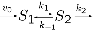
Figure 1: Pathway

Assume mass-action kinetics for each of the reactions. We will model the system with the following parameter values: $v_{0}=4$, $k_{1}=3$, $k_{-1}=0.5$, and $k_{2}=2$. Since the flow into $S_{1}$ is fixed, the system is asymptotically stable to the equilibrium $(S_{1},S_{2})=(\frac{5}{3},2)$. We will consider the unscaled response coefficients defined for initial conditions at the steady state (recall ${\bf R^{s}}(\cdot)$ depends on the nominal parameters values and the initial state). Thus in this case the nominal trajectory will be the steady state trajectory $(S_{1}(t),S_{2}(t))=(\frac{5}{3},2)$ for all $t\geq 0$.

First consider the sensitivity to a perturbation in $k_{1}$ (shown in Figure 2).

Figure 2: Perturbation in $k_{1}$

The steady state response of $S_{2}$ to such a perturbation is nil (since at steady state, $S_{2}=\frac{v_{0}}{k_{2}}$). However, the analysis shows (and intuition concurs), that an increase in $k_{1}$ will produce a transient increase in $S_{2}$, which fades gradually as $S_{1}$ decreases to accommodates the perturbed parameter. The response in $S_{1}$ grows to reach its steady state value – a small overshoot can be seen at about time $t=1$. Not surprisingly, the situation for perturbations in $k_{-1}$ is similar (but reversed), with a transient decrease in $S_{2}$ and a positive steady state response in $S_{1}$ (Figure 3).

Figure 3: Perturbation in $k_{-1}$

One can read from the graphs how the effect on each concentration changes over time. For instance, the effect of these changes on $S_{2}$ is felt most strongly at about $t=0.4$.

Finally, we consider the effect of a perturbation in the initial value of $S_{1}$ (Figure 4).

Figure 4: Perturbation in $S_{1}(0)$

Again, the results are as expected, with transient effects of the perturbations “washing through” the pathway – the result being no effect on the steady state solution.

Having considered the effect of perturbations around a steady state, we now turn our attention to a system whose time-behaviour is more complex.

5.2 Oscillatory Systems

We consider another simple two species pathway, based on a model which has been employed in investigations of glycolytic oscillations [6]. The network is shown in Figure 5.

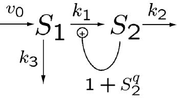
Figure 5: Oscillatory System

The rates are calculated by mass-action, with the activation by $S_{2}$ appearing as a multiplicative factor (i.e. the rate of production of $S_{2}$ is given by $k_{1}S_{1}(1+S_{2}^{q})$). For parameters in a certain range, the concentrations of $S_{1}$ and $S_{2}$ follow oscillatory trajectories; the positive feedback from $S_{2}$ drives the oscillation.

We choose nominal parameter values of $v_{0}=8$, $k_{1}=1$, $k_{2}=5$, $k_{3}=1$, and $q=3$, and nominal initial values of $(S_{1}(0),S_{2}(0))=(1,3)$. The oscillatory behaviour is a limit cycle (cf. [6]), and so any initial conditions in a neighbourhood of these points will yield similar trajectories.

We first consider perturbations in initial values. The limit cycle behaviour is stable; after a perturbation of the initial conditions, the system will tend to the limit cycle as time tends to infinity. However, unlike the previous case where convergence to the same behaviour meant that the response shrank to zero as time moved on, for this model (and for systems with limit cycles in general), the phase of the oscillations depends on the initial values. Thus the perturbed trajectory is out of phase with the nominal trajectory. The result is a periodic response – oscillating with the same period as the limit cycle and indicating the difference in the trajectories at each point in time. The response for perturbations in $S_{1}(0)$ is shown in Figure 6, along with the nominal trajectory.

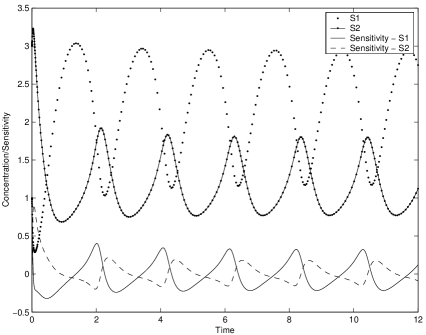
Figure 6: Perturbation in $S_{1}(0)$

The response for perturbations in $S_{2}(0)$ (not shown) is similar.

Care must be taken in extending this set of ideas to perturbations of kinetic parameters of an oscillatory system. In general, the results of such analysis may not be useful. The response coefficients for perturbations in $v_{0}$ are shown (again, along with the nominal trajectories) in Figure 7.

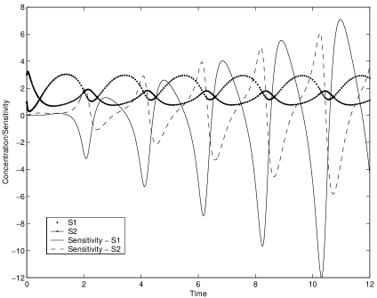
Figure 7: Perturbation in $v_{0}$

While the sensitivities match the period of the system in a quasi-periodic behaviour, they oscillate more and more widely, and continue to do so as time tends to infinity. As a result, these responses are not especially useful when trying to predict the effect of finite perturbations on a real system. The trouble, as pointed out in [4, 11], is that after a perturbation in a kinetic parameter, the system again exhibits a limit cycle behaviour, but this time with a different period. When two trajectories follow a similar cycle with different periods, they will always reach a point when they are completely out of phase, no matter how small the difference in their periods. As the perturbations get smaller, the difference in period shrinks as well, so that it takes longer and longer for this “point of maximum difference” to be reached. However, as long as the perturbation is nonzero, that point will always be achieved. Since the response coefficient is defined as the limit of the ratio of the difference in trajectories to the size of the perturbation as the perturbation goes to zero, we find that as time tends to infinity, the response approaches this “maximum difference” divided by zero, that is it diverges.

In [4] and [11], some clever strategies have been devised for interpreting the sensitivities of oscillatory systems. Kholodenko et al. treat the case of asymptotically stable systems under the influence of periodic external forces in [11]. Such systems exhibit limit cycles whose period is set by the external force. In this case, perturbations in kinetic parameters do not result in changes in the period, and so the response coefficients are more meaningful. In [4], Demin et al. treat perturbations of autonomously oscillating systems by measuring the response in the Fourier coefficients of the trajectory. Fourier control coefficients are introduced, which give a useful interpretation of sensitivities for any periodic systems.

Having considered the interpretation of response coefficients for steady state and oscillating systems, we now treat the most interesting case – a system in which the behaviour of interest occurs during transients.

5.3 Phototransduction

Phototransduction is the process by which organisms convert light signals into nerve signals. As in all signal transduction pathways, the steady state behaviour of the system is less interesting than its transient response. We will illustrate a sensitivity analysis of the single photon response in a simple model of phototransduction loosely based on previous modeling work in [2] and [13].

The response mechanism is modelled as follows. The system is at steady state in the absence of light input. A photon of light activates a rhodopsin molecule to start the system response. Activated rhodopsin (Ra) in turn activates a heterotrimeric G protein (G). The activated G protein $\alpha$-subunit (Ga) dissociates from its beta-gamma subunits ($\beta\gamma$) and then binds with a cGMP phosphodiesterase (PDE) to form the active PDEa-Ga complex. The PDE enzyme catalyzes the degradation of cGMP in the cell. Activation by Ga greatly enhances the catalytic activity of PDE, resulting in a reduction in cellular levels of cGMP. The cGMP-gated ion channels in the cell membrane then close, causing a net efflux of calcium ion (Ca), a net outward current (J), and a corresponding hyperpolarization of the cell’s membrane.

The deactivation phase of the response is modelled as follows. Activated G protein $\alpha$ subunit, either free (Ga) or bound (PDEa-Ga), is converted to the deactivated form (Gd). Finally, the deactivated G protein (Gd) recombines with the beta-gamma subunit ($\beta\gamma$) to form the heterotrimeric G protein (G).

The model incorporates four independent variables (G, Ga, PDEa-Ga, and cGMP) along with five dependent variables (Gd, PDE, $\beta\gamma$, Ca, and J) and several parameters as indicated below. Note, J denotes not the actual current but rather the magnitude of the deviation from the resting current (DarkJ). The input to the system is the time-varying level of Ra. The network is shown in Figure 8.

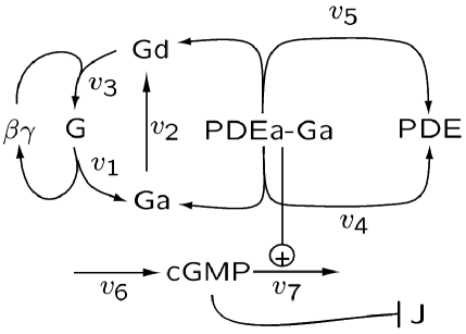
Figure 8: Phototransduction Pathway

The dynamics are given by

$$v_{1} = k_{Ga}\hbox{\rm\ Ra\ \/}$$

$$v_{2} = k_{Gd}\hbox{\rm\ Ga\ \/}$$

$$v_{3} = k_{G1}\hbox{\rm\ $\beta\gamma$ Gd\ \/}$$

$$v_{4} = k_{PDE1}\hbox{\rm\ Ga PDE\ \/}-k_{PDE1m}\hbox{\rm\ PDEa-Ga\ \/}$$

$$v_{5} = k_{PDE2}\hbox{\rm\ PDEa-Ga\ \/}$$

$$v_{6} = \frac{k_{cG}}{1+\left(\frac{\hbox{\rm\ Ca\ \/}}{K_{g}}\right)^{q}}$$

$$v_{7} = k_{cGd0}\hbox{\rm\ cGMP\ \/}+k_{cGd}\hbox{\rm\ cGMP PDEa-Ga\ \/}$$

 Gd $$= \hbox{\rm\ Gtot\ \/}-\hbox{\rm\ G\ \/}-\hbox{\rm\ Ga\ \/}$$

 PDE $$= \hbox{\rm\ PDEtot\ \/}-\hbox{\rm\ PDEa-Ga\ \/}$$

 $$\beta\gamma = \hbox{\rm\ $\beta\gamma$tot\ \/}-\hbox{\rm\ G\ \/}$$

 Ca $$= \frac{k_{C_{i}}}{k_{C_{o}}}\left(\frac{\hbox{\rm\ cGMP\ \/}}{K_{0.5}}\right)^{3}$$

 J $$= \hbox{\rm\ DarkJ\ \/}\left(1-\left(\frac{\hbox{\rm\ cGMP\ \/}}{K_{0.5}}\right)^{3}\right)$$

For simulations, we choose nominal parameter values and initial conditions as follows

$$\begin{array}[]{ll}k_{Ga}=1.0\hbox{\rm\ ms\ \/}\!^{-1}&k_{Gd}=0.005\hbox{\rm\ ms\ \/}\!^{-1}\\ k_{G1}=0.002\hbox{\rm\ ms\ \/}\!^{-1}\hbox{\rm\ molecules\ \/}\!^{-1}\,\mu\!\!\hbox{\rm\ m\ \/}\!\!^{2}&k_{PDE1}=0.0003\hbox{\rm\ ms\ \/}\!^{-1}\hbox{\rm\ molecules\ \/}\!^{-1}\,\mu\!\!\hbox{\rm\ m\ \/}\!\!^{2}\\ k_{PDE1m}=0.000001\hbox{\rm\ ms\ \/}\!^{-1}&k_{PDE2}=0.005\hbox{\rm\ ms\ \/}\!^{-1}\\ k_{cG}=0.058\hbox{\rm\ mM\ \/}\hbox{\rm\ ms\ \/}\!^{-1}&K_{g}=0.2\hbox{\rm\ mM\ \/}\\ q=2.0&k_{cGd0}=0.002\hbox{\rm\ ms\ \/}\!^{-1}\\ k_{cGd}=0.000004\hbox{\rm\ ms\ \/}\!^{-1}\hbox{\rm\ molecules\ \/}\!^{-1}\,\mu\!\!\hbox{\rm\ m\ \/}\!\!^{2}&k_{C_{o}}=1.44\\ k_{C_{i}}=0.72&K_{0.5}=4\hbox{\rm\ mM\ \/}\\ \\ \hbox{\rm\ Gtot\ \/}=3000\hbox{\rm\ molecules\ \/}\mu\!\!\hbox{\rm\ m\ \/}\!\!^{-2}&\hbox{\rm\ PDEtot\ \/}=500\hbox{\rm\ molecules\ \/}\mu\!\!\hbox{\rm\ m\ \/}\!\!^{-2}\\ \hbox{\rm\ $\beta\gamma$tot\ \/}=3000\hbox{\rm\ molecules\ \/}\mu\!\!\hbox{\rm\ m\ \/}\!\!^{-2}\par&\hbox{\rm\ DarkJ\ \/}=12.0\hbox{\rm\ pA\ \/}\\ \\ \hbox{\rm\ G\ \/}\!(0)=3000\hbox{\rm\ molecules\ \/}\mu\!\!\hbox{\rm\ m\ \/}\!\!^{-2}&\hbox{\rm\ Ga\ \/}\!(0)=0\hbox{\rm\ molecules\ \/}\mu\!\!\hbox{\rm\ m\ \/}\!\!^{-2}\\ \hbox{\rm\ PDEa-Ga\ \/}\!(0)=0\hbox{\rm\ molecules\ \/}\mu\!\!\hbox{\rm\ m\ \/}\!\!^{-2}&\hbox{\rm\ cGMP\ \/}\!(0)=4.0\hbox{\rm\ mM\ \/}\end{array}$$

The single activated rhodopsin molecule excited by a single photon is represented by a square 100ms pulse,

$$\hbox{\rm\ Ra\ \/}(t)=\left\{\begin{array}[]{ll}0&0\leq t\leq 100\\ 1&100<t\leq 200\\ 0&200<t\end{array}\right.,$$

measured in$\hbox{\rm\ molecules\ \/}\mu\!\!\hbox{\rm\ m\ \/}\!\!^{-2}$.

We first consider the effect of a perturbation in the parameter $k_{Ga}$, which describes the effect of activated rhodopsin on the activation of G. The nominal trajectories for G, Ga and PDEa-Ga are shown in Figure 9 and Figure 10.

Figure 9: Nominal trajectory for G

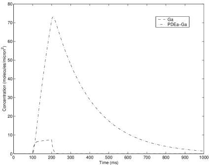
Figure 10: Nominal trajectory for Ga, PDEa-Ga

(There is no activity until time $t=100$ since the system is at steady state while the input is zero). Figure 11

Figure 11: Absolute sensitivities to perturbations in $k_{Ga}$

shows the absolute (unscaled) sensitivity of G, Ga and PDEa-Ga to perturbations in $k_{Ga}$. As expected, an increase in $k_{Ga}$ causes a decrease in the level of G and an increase in the levels of Ga and PDEa-Ga. These responses track the trajectories themselves, with the largest response being observed when each species is farthest from its “resting” (steady) state.

The primary signal of interest in this system is the level of current (J) produced by the input. The time history of the current produced by the nominal input and parameter values is shown in Figure 12.

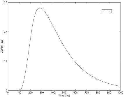
Figure 12: Nominal trajectory of J

The effect of perturbations in three different parameters on J are shown in Figure 13. Since this analysis is meant to compare the effects of the changes, the relative (i.e. scaled) responses are shown.

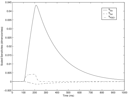
Figure 13: Relative sensitivities of J

The relative strengths of perturbations in the three parameters $k_{Ga}$, $k_{Gd}$ and $k_{PDE1}$ are immediate. For instance, to increase the response in J, it is clear that an increase in $k_{Ga}$ will have far more impact than an equal (relative) increase in $k_{PDE1}$ or decrease in $k_{Gd}$.

6 Conclusion

Since its introduction, Metabolic Control Analysis has proven to be a useful tool in discovering the distribution of control in biochemical systems at steady state. In this paper, the computation and interpretation of system sensitivities has been considered for arbitrary trajectories. The main results of MCA (Summation and Connectivity Theorems) have been shown to have a valid interpretation not just at steady state, but throughout the system dynamics. In analyzing the distribution of control for systems in which transients are of interest, the time varying sensitivity may prove to be a valuable tool in determining system behaviour.

Acknowledgment The authors would like to thank Tau-Mu Yi for providing the phototransduction model and for many useful discussions.

Appendix A Appendix: A Primer on Operators

A function from ${\mathbb{R}}$ into ${\mathbb{R}}$ is defined as a rule which assigns to each real number a unique real number in its range, for example, the function $h(\cdot)$ defined by $h(t)=t^{2}$ for each $t\in{\mathbb{R}}$. This can be generalized by allowing functions to act on pairs of numbers, or $n$-tuples in general (e.g. $g(x,y,z)=x^{2}-yz$).

The concept of a function can be extended to yield an operator, which takes a function as its argument. For example, we could consider the operator $T(\cdot)$ defined by integration:

$$T(f(\cdot))=\int_{0}^{1}f(s)\,ds$$

for each function $f(\cdot)$ defined on ${\mathbb{R}}$ (provided the integral of $f$ exists). Define the functions $h$ and $r$ by $h(t)=t^{2}$ and $r(t)=\cos(t)$. Then

$$T(h(\cdot))=\int_{0}^{1}s^{2}\,ds=\frac{1}{3},\qquad\hbox{\rm\ and\ \/}\qquad T(r(\cdot))=\int_{0}^{1}\cos(s)\,ds=\sin(1).$$

Another example of an operator is function evaluation. Define $G$ by $G(f(\cdot))=f(5)$ for each function $f(\cdot)$. Then $G(h(\cdot))=25$ and $G(r(\cdot))=\cos(5)$.

The operators $T$ and $G$ defined above are commonly referred to as functionals, since they map functions to numbers. More generally, by allowing an operator to have a second, scalar argument, we can construct operators which map functions to functions. For example, extending $T$ to depend on a scalar argument $t$, we could define $\widehat{T}$ by

$$\widehat{T}(t,f(\cdot))=\int_{0}^{t}f(s)\,ds.$$

An alternative notation is $\widehat{T}(t)(f(\cdot))=\widehat{T}(t,f(\cdot))$. Thus, given a real-valued function, $T$ returns a function defined for $t\geq 0$:

$$T(t)(h(\cdot))=\int_{0}^{t}s^{2}\,ds=\frac{t^{3}}{3}\qquad\hbox{\rm\ and\ \/}\qquad T(t)(r(\cdot))=\int_{0}^{t}\cos(s)\,ds=\sin(t).$$

As another example, we could modify $G$ by defining $\widehat{G}(t)(f(\cdot))=f(2t)$. Then $\widehat{G}(t)(h(\cdot))=(2t)^{2}$ and $\widehat{G}(t)(r(\cdot))=\cos(2t)$, for all $t\in{\mathbb{R}}$.

As described in the main text, we can extend the action of operators to row vectors in a component-wise fashion, for example

$$\widehat{T}(t)([\begin{array}[]{cc}h(\cdot)&r(\cdot)\end{array}])=[\begin{array}[]{cc}\frac{t^{3}}{3}&\sin(t)\end{array}].$$

Moreover, we can combine operators column-wise, yielding the notation

$$\left[\begin{array}[]{c}\widehat{T}(t)\\ \widehat{G}(t)\end{array}\right]([\begin{array}[]{cc}h(\cdot)&r(\cdot)\end{array}])=\left[\begin{array}[]{cc}\frac{t^{3}}{3}&\sin(t)\\ (2t)^{2}&\cos(2t)\end{array}\right].$$

Particular cases of operator actions which appear in the main text are:

• constant functions as arguments to operators. For example, defining the function $k(\cdot)$ by $k(t)=3$ for all $t\in{\mathbb{R}}$, we have

  $$T(k(\cdot))=3,\ \ \widehat{T}(t)(k(\cdot))=3t.$$

  Using a simplified notation, we can write

  $$T(3)=3,\ \ \widehat{T}(t)(3)=3t;$$

• operators which act by multiplication. For example, define the operator $H$ by $H(t)(f(\cdot))=3tf(t)$. Then

  $$H(t)(h(\cdot))=3t^{3}\ \ \ \ \ H(t)(r(\cdot))=3t\cos(t)\ \ \ \ \ H(t)(3)=9t.$$

References

- [1] Acerenza, L., Sauro, H. M. and Kacser, H., “Control analysis of time-dependent metabolic systems,” Journal of Theoretical Biology, 151 (1989), pp. 423–444.
- [2] Rieke, F. and Baylor, D. A., “Origin of reproducibility in the responses of retinal rods to single photons,” Biophysical Journal, 75 (1998), pp. 1836–1857.
- [3] Boyce, W. E. and DiPrima, R. C., Elementary Differential Equations and Boundary Value Problems, Fifth Edition, John Wiley & Sons, New York, 1992.
- [4] Demin, O. V., Westerhoff, H. V. and Kholodenko, B. N., “Control analysis of stationary fixed oscillations,” Journal of Physical Chemistry B, 103 (1999), pp. 10695–10710.
- [5] Fell, D.A., “Metabolic control analysis – a survey of its theoretical and experimental development,” Biochemical Journal, 286 (1992), pp. 313–330.
- [6] Heinrich, R., Rapoport, S. M. and Rapoport, T. A., “Metabolic regulation and mathematical models,” Progress in Biophysics & Molecular Biology, 32 (1977), pp. 1–82.
- [7] Heinrich, R. and Reder, C., “Metabolic control analysis of relaxation processes,” Journal of Theoretical Biology, 151 (1991), pp. 343–350.
- [8] Heinrich, R. and Schuster, S., The Regulation of Cellular Systems, Chapman & Hall, New York, 1996.
- [9] Hofmeyr, J-H. S., “Metabolic control analysis in a nutshell,” Proceedings of the International Conference on Systems Biology, Pasadena, California, November 2000, pp. 291–300.
- [10] Kascer, H. and Burns, J. A., “The control of flux”, Symp. Soc. Exp. Biol., 27 (1973), pp. 65-104.
- [11] Kholodenko, B. N., Demin, O. V. and Westerhoff, H. V., “Control analysis of periodic phenomena in biological systems,” Journal of Physical Chemistry B, 101 (1997), pp. 2070–2081.
- [12] Kohn, M. C., Whitley, L. M. and Garfinkel, D., “Instantaneous flux control analysis for biochemical systems,” Journal of Theoretical Biology, 76 (1979), pp. 437–452.
- [13] Pugh, Jr., E. N. and Lamb, T. D., “Amplification and kinetics of the activation steps in phototransduction,” Biochemica et Biophysica Acta, 1141 (1993), pp. 111–149.
- [14] Reder, C., “Metabolic control theory: a structural approach,” Journal of Theoretical Biology, 135 (1988), pp. 175–201.
- [15] Reijenga, K. A., Westerhoff, H. V., Kholodenko, B. N. and Snoep, J. L., “Control analysis for autonomously oscillating biochemical networks,” Biophysical Journal, 82 (2002), pp. 99–108.
- [16] Sauro, H. M., “Jarnac: A system for interactive metabolic analysis,” in Animating the Cellular Map: Proceedings on BioThermoKinetics, Hofmeyr, J.-H. S., Rohwer, J. M. and Snoep, J. L., eds., Stellenbosch University Press, 2000.
- [17] Savageau, M.A., Biochemical Systems Analysis. A Study of Function and Design in Molecular Biology, Addison-Wesley, Reading, MA.
- [18] Tomović, R., Sensitivity Analysis of Dynamic Systems, McGraw-Hill, New York, 1963.