Chaotic Behavior of Positronium
in a Magnetic Field.

Abstract

Classical motion of positronium embedded in a magnetic field is studied, and computation shows the emergence of chaotic orbits. Recent work investigating quantum behavior of this system predicts extremely long lifetimes jA97 jS98 . Chaos assisted tunneling however may lead to significant shortening of the lifetime of this system.

Two interacting charged particles placed in a magnetic field exhibit chaotic motion. This has been studied for the hydrogen and Rydberg atom jD84 and the scattering of electrons on positive nuclei gS00 .This has an impact on the electrical conductivity of fully ionized plasmas gS02 bH02 .

Here we study the classical motion of positronium in a magnetic field. In the absence of a magnetic field the positronium has a very short lifetime. It was found by Ackermann et. al.jA97 that in a strong magnetic field the positronium can have an extremely long lifetime ”up to the order of one year”jA97 .

We find that the classical motion is chaotic, which usually leads to chaos assisted tunneling pt01 which should significantly reduce the lifetime of this system.

The calculation includes the case of crossed electric and magnetic fields, provided that the ratio of the field strengths $E/B$ does not exceed the speed of light. In this case the electric field can be eliminated by a Lorentz transformation.

The motion of two particles with charges  +e and  -e of equal mass m moving, in a uniform magnetic field $\ \mathbf{B}$ are described by the equations

$${m}\bm{\ddot{r}}_{1}=\allowbreak e\bm{\dot{r}}_{1}\times\bm{B}-\frac{e^{2}}{4\pi\epsilon_{0}}\frac{\bm{r}_{1}-\bm{r}_{2}}{\mid\bm{r}_{1}-\bm{r}_{2}\mid^{3}}$$ (1)

$${m}\bm{\ddot{r}}_{2}=-e\bm{\dot{r}}_{2}\times\bm{B}+\frac{e^{2}}{4\pi\epsilon_{0}}\frac{\bm{r}_{1}-\bm{r}_{2}}{\mid\bm{r}_{1}-\bm{r}_{2}\mid^{3}}$$ (2)

Adding (1) and (2) gives

$${m}(\bm{\ddot{r}}_{1}+\bm{\ddot{r}}_{2})=e(\bm{\dot{r}}_{1}-\bm{\dot{r}}_{2})\times\bm{B}$$ (3)

Introducing the new coordinates

$$\bm{r}_{1}+\bm{r}_{2}=\bm{R}$$ (4)

$$\bm{r}_{1}-\bm{r}_{2}=\bm{r}$$ (5)

and integrating Eq. (3) results in

$${m}\bm{\dot{R}}-e\bm{r}\times\bm{B}=\bm{\alpha}$$ (6)

where $\bm{\alpha}$ is a constant vector. Subtracting Eq.(2) from (1) gives

$${m}\bm{\ddot{r}}=e\bm{\dot{R}}\times\bm{B}-\frac{e^{2}\bm{r}}{2\pi\epsilon_{0}r^{3}}$$ (7)

and using Eq.(6)

$${m}\bm{\ddot{r}}=\frac{e}{m}(e\bm{r}\times\bm{B}+\bm{\alpha})\times\bm{B}-\frac{e^{2}}{2\pi\epsilon_{0}}\frac{\bm{r}}{r^{3}}$$ (8)

Introducing the cyclotron frequency $\ \omega_{c}=eB/m,$ and choosing $\bm{B}$ pointing in the z direction $\bm{B}=B\bm{e}_{3},$ Eqs. (8) and (6) become

$$\bm{\ddot{r}}/\omega_{c}^{2}=(\bm{r}\times\bm{e}_{3})\times\bm{e}_{3}+\bm{\alpha}\times\bm{e}_{3}/(eB)-\frac{m}{2\pi\epsilon_{0}B{{}^{2}}}\frac{\bm{r}}{r{{}^{3}}}$$ (9)

$$\bm{\dot{R}}/\omega_{c}-\bm{r}\times\bm{e}_{3}=\bm{\alpha}/eB$$ (10)

With the dimensionless variables $\ \omega_{c}t\rightarrow t$ and  $r(2\pi\epsilon_{0}B{{}^{2}}/m)^{1/3}\rightarrow r,$ one arrives to the dimensionless equations of motion

$$\bm{\ddot{r}}=(\bm{r}\times\bm{e}_{3})\times\bm{e}_{3}+\bm{\alpha}^{{}^{\prime}}\times\bm{e}_{3}-\bm{r}/r{{}^{3}}$$ (11)

$$\bm{\dot{R}}-\bm{r}\times\bm{e}_{3}=\bm{\alpha}^{{}^{\prime}}$$ (12)

where $\ \bm{\alpha}^{{}^{\prime}}=\bm{\alpha}/eB$ is the dimensionless constant vector. Since $\bm{r}\times\bm{e}_{3}$ has no component in the z direction, it is convenient to chose a coordinate system where the initial value  of $\dot{R}_{z}(0)=0$, so the constant $\ \bm{\alpha}^{{}^{\prime}}$ is a vector in the $x-y$ plane, $\bm{\alpha^{{}^{\prime}}}=a\bm{e}_{1}+b\bm{e}_{2}.$Without loss of generality one may chose either a=0 or b=0. So Eq.(11)  becomes

$$\bm{\ddot{r}}+\bm{r}_{\perp}=-\bm{r}/r{{}^{3}}+b\bm{e}_{1}$$ (13)

where $\bot$ means perpendicular to the z axis.

First we study the two dimensional case

$$\begin{array}[]{l}\ddot{x}+x=-x/r{{}^{3}}+b\\ \ddot{y}+y=-y/r{{}^{3}}\end{array}$$ (14)

with the Hamiltonian

$$H=p{{}^{2}}/2+r{{}^{2}}/2-1/r-bx$$ (15)

Since energy is conserved phase space is three dimensional. The potential energy  $V=r^{2}/2-1/r-bx$ is singular at $\ r\rightarrow 0,$ and develops a minimum when $b\geq 1.89$. 1 shows equipotential lines for b=3. Surface of section plots in the $x,p_{x}$ plane have been computed for different values of the two parameters: b and the energy E.2.ashows four plots, $E=0,b=1$ $and$ $b=3;E=-.5,b=1$ and $3.$ The plots appear regular without any chaotic orbits. We have carried out many more computations for different values of  E and b with similar results. It appears therefore that an additional constant of motion exists, but the analytic expression has not been found. We have also carried out computations to find the largest Lyapunov exponent which turned out to be zero as expected for non-chaotic orbits.

Turning to the three dimensional case we study the $\bm{\alpha=}0$ limit. in this case it is convenient to introduce polar coordinates where the system is described by the Hamiltonian

$$H=P_{\rho}^{{}^{2}}/2+P_{z}^{2}/2+P_{\varphi}^{2}/(2\rho^{2})+\rho^{2}/2-1/\sqrt{\rho^{2}+z^{2}}$$ (16)

where $\rho^{2}=x^{2}+y^{2}$ , and  $\varphi$ is an ignorable coordinate so  $P_{\varphi}=const.$ This gives the equations of motion

$$\begin{array}[]{l}\frac{\partial H}{\partial P_{\rho}}=\dot{\rho}\\[10.0pt] \frac{\partial H}{\partial P_{z}}=\dot{z}\\[10.0pt] \dot{P}_{\rho}=-\frac{\partial H}{\partial\rho}=-\rho+P_{\varphi}^{2}/\rho^{3}-\frac{\rho}{(\rho^{2}+z^{2})^{3/2}}\\[10.0pt] \dot{P}_{z}=-\frac{\partial H}{\partial z}=-\frac{z}{(\rho^{2}+z^{2})^{3/2}}\end{array}$$ (17)

A surface of section plot ($\rho,P_{\rho})$ in the z=0 plane is shown in 3 for E=-.5, $P_{\varphi}=.25$. The existence of chaotic orbits is obvious, so the three dimensional equations of motion are not integrable. To show that chaotic orbits exist  for $\bm{\alpha\neq}0$, the largest Lyapunov exponent has been computed for the three dimensional case for b=3, as shown in 4, using the algorithm as described in Ref.eO93 It converges to a value larger then zero as expected.

In conclusion the motion of positronium immersed in a magnetic field is chaotic in the classical limit, therefore the long lifetime predicted in the quantum limit is unlikely.

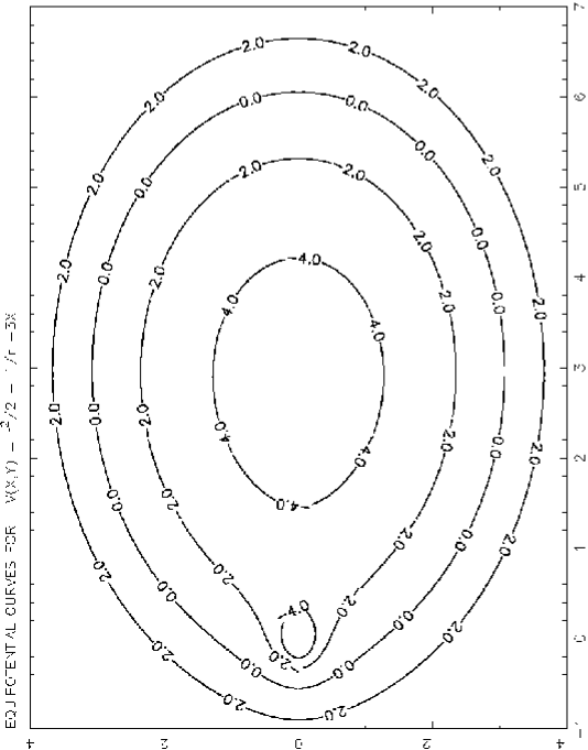
Figure 1: Equipotential curves for the two dimensional case with b=3

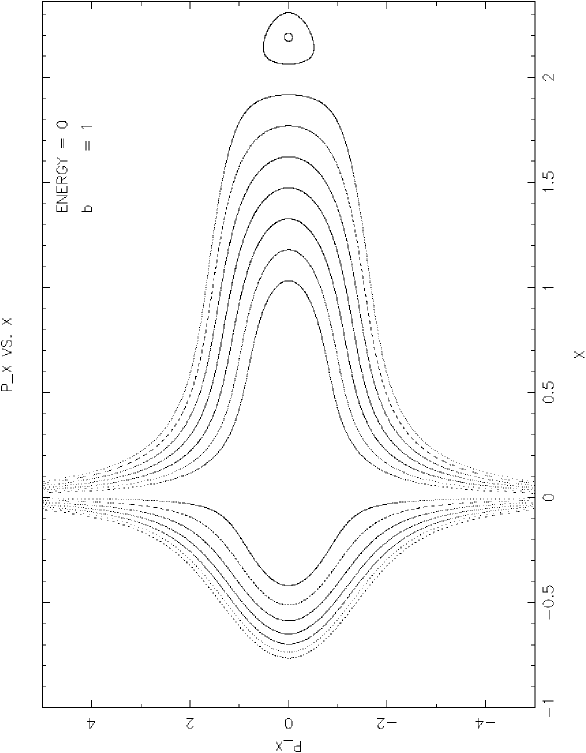
Figure 2.a: Surface of section plots in the $x-p_{x}$ plane,E=0,b=1

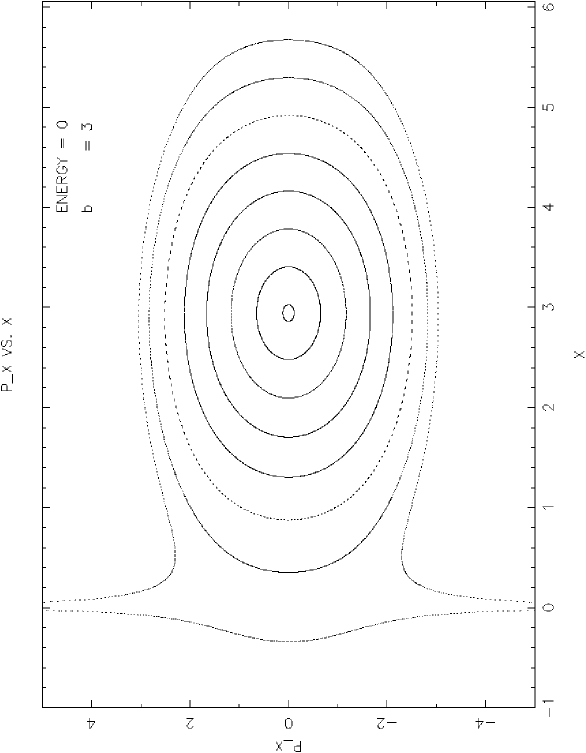
Figure 2.b: E =0,b = 3

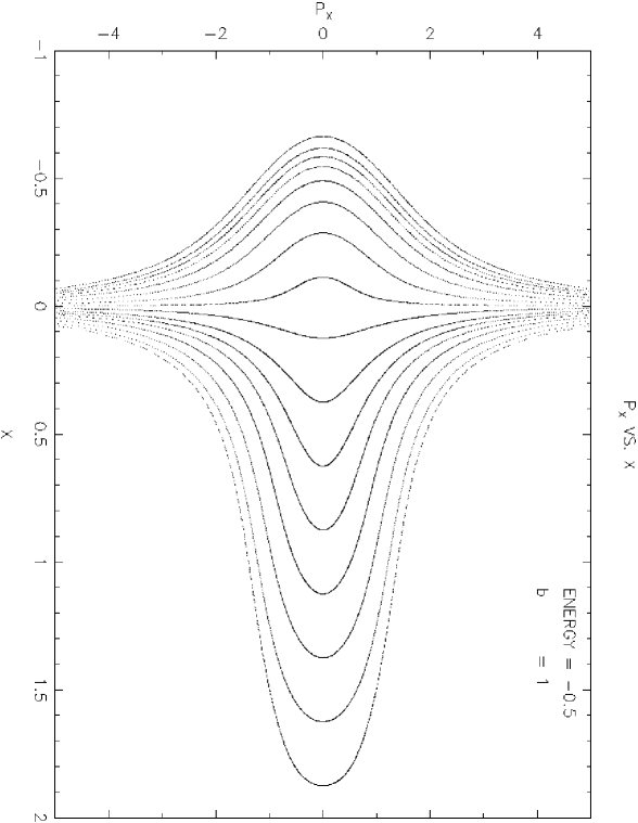
Figure 2.c: E = -0.5, b = 1

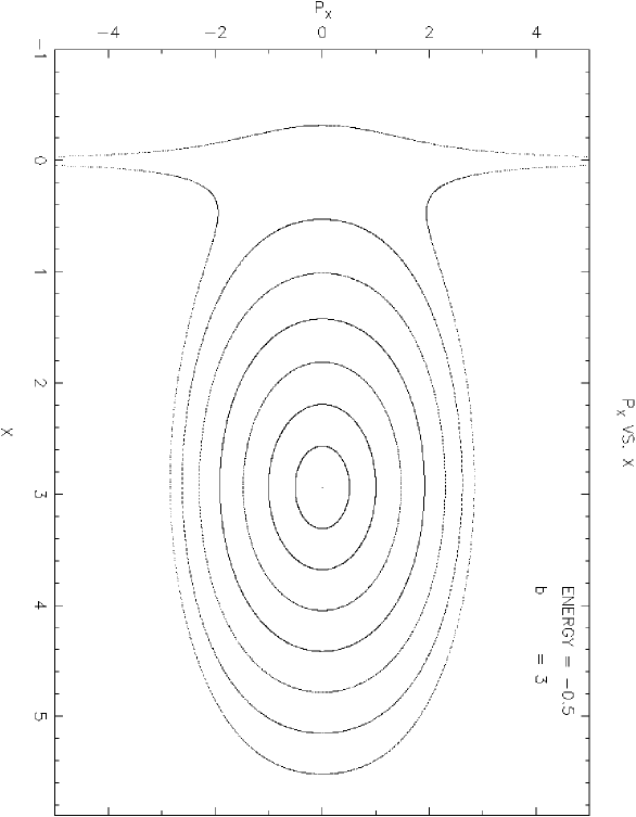
Figure 2.d: E = -0.5, b = 3

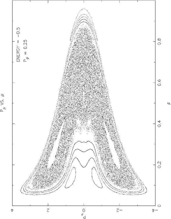
Figure 3: Surface of sections plot for the three dimensional case, where b= 0 in the $\rho-P_{\rho}$ plane

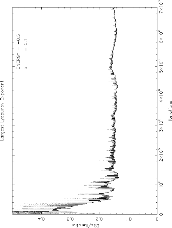
Figure 4: Computation of the largest Lyapunov exponent, E=-0.5, b=0.1 with initial conditions
$x_{1}$ = 0.65,$y_{1}$ = 0.0,$z_{1}$ = 0.0
$P_{x1}$ = 0.0,$P_{y1}$ = 0.25,$P_{z1}$ = 1.31222067
$x_{2}$ = 0.65000001,$y_{2}$ = 0.0,$z_{2}$ = 0.0
$P_{x2}$ = 0.0,$P_{y2}$ = 0.25,$P_{z2}$ = 1.31222064

References

(1)
J.B.Delos,S.K.Knudson,D.W. Noid,
Phys. Rev. A 30, 1208 (1984)
(2)
G. Schmidt,E.E. Kunhardt,J. Godino,
Phys. Rev.E 62,7512 (2000).
(3)
G. Schmidt,
Comments on Modern Physics to appear.
(4)
B. Hu, W. Horton, C. Chiu and T. Petrovsky,
Physics of Plasmas to appear.
(5)
J.Ackermann, J. Shertzer and P. Schmelcher,
Phys. Rev. Letters.78, 199(1997).
(6)
J.Schertzer, J. Ackermann and P. Schmelcher,
Phys. Rev. A.58,1129 (1998).
(7)
Physics Today, Aug 2001, p. 13 and references therein.
(8)
E. Ott,
Chaos in Dynamical Systems,
Cambridge University Press 1993. p.129.