Fluctuation of the ambipolar equilibrium in magnetic perturbations

Abstract

We draw attention on the fast oscillatory deviations from the residual non-ambipolarity in the case where electrons are driven by strong magnetic perturbations.

If the turbulent diffusion of the electrons and ions are different one can expect that a radial electric field develops (such that the ambipolarity is reinstored) and that poloidal plasma spin-up can occur. However it has been shown that the diffusion of particles in turbulent fields is ambipolar. In Ref.[1] the difference in the radial fluxes generated by fluctuating fields has been considered and the rôle of the ion polarization drift has been underlined. The radial ion flux partially cancels the radial electron flux and the ambipolarity is reestablished approximately, to the order $1/\varepsilon_{\perp}$, which is a very small quantity ($\varepsilon_{\perp}$ is the plasma transversal permitivity constant). The problem has been examined in detail for instabilities having a substantial magnetic component in Ref.[2]. When the unstable modes that drive the radial transport are bounded inside plasma (i.e. it can be assumed that there is no exchange of momentum with the region outside plasma) the fluxes are ambipolar in average over a spatial region including several mode-resonance surfaces. Pointwise non-zero radial currents, even reduced by the fraction $1/\varepsilon_{\perp}$, are able to build up charge filaments and can cause the plasma to be Kelvin Helmholtz unstable.

We return to this problem to examine a situation where the non-ambipolarity is switched on by an external source acting on the electron component. We assume that the electrons are radially driven by a magnetic perturbation which imposes a constant radial flux starting at $t=0$. The ion polarization drift re-establishes the equality of the fluxes (to order $1/\varepsilon_{\perp}$) but in this particular case a stationary equilibrium cannot be reached. The existence of a radial non-zero current yields a non-zero time derivative of the radial electric field, i.e. a non-zero time derivative of the poloidal velocity. The plasma would be accelerated without limit in the poloidal direction, but the torque competes with the magnetic pumping, a very effective damping mechanism. We draw attention to the oscillatory variation of the velocity, which occurs an a scale much faster than the dissipative decay.

Such “events”, consisting of sudden creation of non-ambipolar fluxes, followed by a fast plasma response in view of reinstoring the ambipolarity, can appear in a random space and time sequence and on the average can affect the plasma dynamics. To look in detail to only one event we shall adopt an “initial value” point of view. We consider the slab geometry with $x$ the radial coordinate increasing from the reference point toward the centre of plasma, $y$ the poloidal coordinate, $z$ is directed along the shearless magnetic field such as the mixed product of the three versors is positive. The radial electric current is switched on at $t=0$ , $j_{x}\left(t=0\right)=-env_{x}^{e}$ (we note $e\equiv\left|e\right|$) and for simplicity we shall assume that $v_{x}^{e}$ is constant in time and uniform in space during this single event. From the momentum conservation we find (with $c$ and $v_{A}$ respectively the light speed and the Alfven speed),

$$-env_{x}^{e}\approx B_{z}\varepsilon_{0}\left(1+\frac{c^{2}}{v_{A}^{2}}\right)\left(\frac{\partial v_{y}^{i}}{\partial t}\right)$$ (1)

We have neglected the damping and the diamagnetic flow. From the initial non-ambipolar current $(-env_{x}^{e}=j_{x}\left(0\right)\neq 0)$ it results a time-growing poloidal velocity whose magnitude is inverse proportional to the very large factor representing the plasma transversal permitivity $\varepsilon_{\perp}=1+c^{2}/v_{A}^{2}$.

Since the time-derivative of the poloidal velocity is constant, the plasma rotates indefinitely in the poloidal direction with higher and higher velocity. Naturally this requires the consideration of saturation mechanisms and makes desirable a time-depending investigation. We write in more detail the ion momentum equations on $x$ and $y$

$$v_{y}^{i}=-\frac{E_{x}}{B_{z}}+\frac{m_{i}}{eB_{z}}\left(\frac{\partial v_{x}^{i}}{\partial t}\right)$$ (2)

$$v_{x}^{i}=-\frac{1}{\Omega_{i}}\left(\frac{\partial v_{y}^{i}}{\partial t}\right)\left[1+\frac{1}{\Omega_{i}}\left(\frac{\partial v_{y}^{i}}{\partial x}\right)\right]^{-1}$$ (3)

$$E_{x}=-B_{z}v_{y}^{i}+\frac{m_{i}}{e}\left(\frac{\partial v_{x}^{i}}{\partial t}\right)$$ (4)

The charge conservation gives

$$0=j_{x}+\varepsilon_{0}\frac{\partial E_{x}}{\partial t}$$ (5)

where

$$j_{x}\left(t\right)=-env_{x}^{e}+env_{x}^{i}$$ (6)

From these relations and using Eqs.(2-4) and (5-6) we obtain a single equation for the poloidal ion velocity.

$$-env_{x}^{e}\Theta\left(t\right) = \frac{en}{\Omega_{i}}\left(\frac{\partial v_{y}^{i}}{\partial t}\right)\frac{1}{U}+\varepsilon_{0}B_{z}\left(\frac{\partial v_{y}^{i}}{\partial t}\right)$$

$$+\frac{\varepsilon_{0}m_{i}}{e\Omega_{i}}\left(\frac{\partial^{3}v_{y}^{i}}{\partial t^{3}}\right)\frac{1}{U}-\frac{2\varepsilon_{0}m_{i}}{e\Omega_{i}^{2}}\left(\frac{\partial^{2}v_{y}^{i}}{\partial t^{2}}\right)\left(\frac{\partial^{2}v_{y}^{i}}{\partial x\partial t}\right)\frac{1}{U^{2}}$$

$$-\frac{2\varepsilon_{0}m_{i}}{e\Omega_{i}^{3}}\left(\frac{\partial v_{y}^{i}}{\partial t}\right)\left(\frac{\partial^{2}v_{y}^{i}}{\partial x\partial t}\right)^{2}\frac{1}{U^{3}}-\frac{\varepsilon_{0}m_{i}}{e\Omega_{i}^{2}}\left(\frac{\partial v_{y}^{i}}{\partial t}\right)\left(\frac{\partial^{3}v_{y}^{i}}{\partial x\partial t^{2}}\right)\frac{1}{U^{2}}$$

where $\varepsilon_{0}$ is the vacuum permitivity, $\Theta\left(t\right)$ is the Heaviside function and

$$U\equiv 1+\frac{1}{\Omega_{i}}\left(\frac{\partial v_{y}^{i}}{\partial x}\right)$$

This equation contains higher time and space $\left(x\right)$ derivatives. In order to simplify the problem we assume that the externally imposed electron flux is uniform on the radial direction (for the region of interest) and this renders the entire model invariant to translation in $x$ coordinate. Then we shall restrict this discussion to solutions which are independent of $x$. We shall neglect the problem of the stability of the uniform solutions at perturbations in $x$. Then we have

$$-v_{x}^{e}\Theta\left(t\right)=\left(b_{1}+b_{2}\right)w+b_{3}\stackrel{{\scriptstyle\cdot\cdot}}{{w}}$$

Here

$$w\left(t\right)\equiv\frac{\partial v_{y}^{i}}{\partial t}$$

The quantities appearing in the equation have been non-dimensionalized: $t\rightarrow t^{\prime}=t/\tau$, $y\rightarrow y^{\prime}=y/l$, $v\rightarrow v^{\prime}=v/v_{0}$, where we take as units: $\tau=\Omega_{i}^{-1}$, $l=\rho_{s}$ the ion Larmor radius at the electron temperature, $v_{0}=\beta v_{th}^{e}$ where $\beta$ is the radial magnetic perturbation $\widetilde{B}_{x}$ normalised to the main magnetic field, $\beta=\widetilde{B}_{x}/B$. $v_{th}^{e}$ is the electron thermal velocity. Finally we remove the primes. The dots means derivative to the time variable. Then the coefficients are

$$b_{1}=\frac{1}{\Omega_{i}}\frac{1}{\tau}$$

$$b_{2}=\frac{\varepsilon_{0}B_{z}}{en}\frac{1}{\tau}$$

$$b_{3}=\frac{\varepsilon_{0}m_{i}}{e^{2}n\Omega_{i}}\frac{1}{\tau^{3}}$$

The solution is obtained by Laplace transform and it reads

$$w\left(t\right) = \frac{-v_{x}^{e}}{b_{1}+b_{2}}+\left(w_{0}-\frac{-v_{x}^{e}}{b_{1}+b_{2}}\right)\cos\left[\left(\frac{b_{1}+b_{2}}{b_{3}}\right)^{1/2}t\right]$$

$$+w_{1}\left(\frac{b_{3}}{b_{1}+b_{2}}\right)^{1/2}\sin\left[\left(\frac{b_{1}+b_{2}}{b_{3}}\right)^{1/2}t\right]$$

The initial conditions are given for the first and the second derivatives of the velocity, respectively $w_{0}$, and $w_{1}$. In physical units

$$w_{0}=-v_{x}^{e}\frac{en}{\varepsilon_{0}B_{z}}$$

$$w_{1}=0$$

The frequency of the oscillations is in physical units

$$\nu_{osc} = \left(\frac{b_{1}+b_{2}}{b_{3}}\right)^{1/2}=\left(\frac{e^{2}n}{\varepsilon_{0}m_{i}}+\Omega_{i}^{2}\right)^{1/2}$$

$$= \Omega_{i}\left(1+\frac{nm_{i}}{\varepsilon_{0}B_{z}^{2}}\right)^{1/2}$$

$$= \Omega_{i}\varepsilon_{\perp}^{1/2}$$

Now we include the effect of the damping due to the magnetic pumping, $\left(\frac{\partial v_{y}^{i}}{\partial t}\right)_{MP}=-\nu v_{y}^{i}$, where $\nu$ is the appropriate decay rate [3], [5], [4]. The equation restricted to the time domain is now

$$-v_{x}^{e}\Theta\left(t\right)=d_{0}v_{y}^{i}+d_{1}\left(\frac{\partial v_{y}^{i}}{\partial t}\right)+d_{2}\left(\frac{\partial^{2}v_{y}^{i}}{\partial t^{2}}\right)+d_{3}\left(\frac{\partial^{3}v_{y}^{i}}{\partial t^{3}}\right)$$

where $\Theta\left(t\right)$ is the Heaviside function and

$$d_{0}=\frac{\nu}{enB_{z}},\;\;\;d_{1}=\frac{1}{\Omega_{i}}+\frac{\varepsilon_{0}B_{z}}{en}$$

$$d_{2}=\frac{\varepsilon_{0}\nu}{e^{2}n^{2}\Omega_{i}},\;\;\;d_{3}=\frac{\varepsilon_{0}m_{i}}{e^{2}n\Omega_{i}}$$

The solution of the equation is obtained by the Laplace transform and is written

$$v\left(t\right) = v_{0}\Theta\left(t\right)+v_{1}q\frac{d_{3}}{d_{0}}+\frac{v_{1}c}{\gamma}\exp\left(\gamma t\right)+$$

$$+2v_{1}\left(-\frac{d_{3}\gamma}{d_{0}}\right)\exp\left(\alpha_{r}t\right)\left[\left(a_{r}\alpha_{r}+a_{i}\alpha_{i}\right)\cos\left(\alpha_{i}t\right)-\left(a_{i}\alpha_{r}-a_{r}\alpha_{i}\right)\sin\left(\alpha_{i}t\right)\right]$$

Here $\alpha$, $\beta=\alpha^{\ast}$ and $\gamma$ are respectively the two complex conjugate and the real roots of the polynomial equation $s^{3}+\left(d_{2}/d_{3}\right)s^{2}+\left(d_{1}/d_{3}\right)s+\left(d_{0}/d_{3}\right)=0$. We have for the real $\left(r\right)$ and imaginary $\left(i\right)$ parts:

$$\alpha_{r}=-\frac{d_{2}}{2d_{3}}-\frac{\gamma}{2}$$

$$\alpha_{i}=\left[-\frac{d_{0}}{d_{3}\gamma}-\left(\frac{d_{2}}{2d_{3}}+\frac{\gamma}{2}\right)^{2}\right]^{1/2}$$

The notations are

$$c=\frac{\gamma\beta}{\left(\alpha-\beta\right)\left(\beta-\gamma\right)}\left[-1-\frac{\alpha}{\beta}-\frac{q\alpha d_{3}}{d_{0}}-\frac{p}{\beta}-\frac{d_{2}}{\beta d_{3}}\right]$$

$$b=\frac{\beta\gamma}{\left(\alpha-\beta\right)\left(\gamma-\beta\right)}\left[-1-\frac{\alpha}{\gamma}-\frac{p}{\gamma}-\frac{q\alpha d_{3}}{d_{0}}-\frac{d_{2}}{\gamma d_{3}}\right]$$

and $a=1-b-c$.

$$p=\frac{d_{2}v_{1}+d_{3}v_{2}}{d_{3}v_{1}}$$

$$q=\frac{-v_{x}^{e}-d_{0}v_{0}}{d_{3}v_{1}}$$

The initial order $i$-derivatives of the velocity are noted $v_{i}$, $i=0,1,2$. They are taken to reflect the sudden onset of the electron flux, i.e. the initial poloidal velocity is zero, $v_{0}\equiv v_{y}^{i}\left(t=0\right)=0$ and the first derivative is obtained from the assumption that at $t=0$ the ions did not yet moved radially ($v_{x}^{i}=0$) which means that

$$v_{1}\equiv\left.\left(\frac{\partial v_{y}^{i}}{\partial t}\right)\right|_{t=0}=\left(-v_{x}^{e}\right)\left(\frac{1}{\Omega_{i}}+\frac{\varepsilon_{0}B_{z}}{en}\right)^{-1}$$

The second derivative is taken zero, $v_{2}=0$. The asymptotic value of the poloidal velocity is insensitive to this parameter.

1 Discussion

The most interesting aspect of this solution is the oscillatory behaviour which is strongly controlled by the non-dissipative part of the equation (i.e. terms not depending on $\nu$). The dynamic is very clear: just at $t=0$ the ions acquire a high time derivative of their poloidal velocity, imposed by $j_{x}\left(t=0\right)=-env_{x}^{e}$. The velocity $v_{y}^{i}$ starts from zero and grows very fast to values which can be higher than those required to cancel the non-ambipolar current $j_{x}$. Then they reverse the current and since the electrons are constrained to follow the external drive (magnetic radial perturbation), the tendency of rotation reverses and so on. The decay due to the magnetic pumping appears on longer time scales and this indeed reduces the plasma rotation, without completely eliminating the oscillations. A plot, Fig. (1) of this evolution is shown, on very large time scale (useful to see the atenuation).

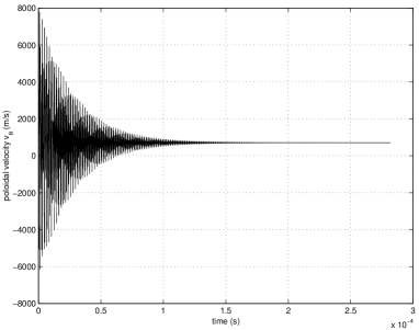
Figure 1: Time variation of the poloidal velocity

The asymptotic value of the poloidal velocity is (with our choices of initial conditions)

$$v_{y}^{i}\left(t\gg\gamma^{-1}\right)=\left(-v_{x}^{e}\right)enB_{z}\nu^{-1}$$

We can see that the nature of these oscillations is similar to that caused by a deviation form electric neutrality, when the frequency is the plasma frequency $\omega_{p}=\left(e^{2}n/\varepsilon_{0}m_{e}\right)^{1/2}$. The important effect of the of these oscillation is in the energy balance. The plasma rotation takes energy from the source of the initial magnetic perturbation and from the electron kinetic energy, since both support the radial electron current. This energy is dissipated via the collisional ion viscosity represented by the magnetic dumping. A more complex treatment of this problem should include a detailed electron dynamics, under the effect of the external magnetic perturbation (which must be quantified). However, the presence of an oscillatory behaviour is still expected and suggests to take this into account when the efficiency of magnetic stochasticity-induced transport is considered.

Acknowledgments Useful discussions with J. H. Misguich and R. Balescu are gratefully acnkowledged.

References

• [1] S. Inoue, T. Tange, K. Itoh and T. Tuda, Nucl. Fusion 19, 1252 (1979).
• [2] R. E. Waltz, Phys. Fluids 25, 1269 (1982).
• [3] A.B. Hassam and R.M. Kulsrud, Phys. Fluids 21, 2271 (1978).
• [4] K.C. Shaing and S. P. Hirschman, Phys. Fluids B1 (1989) 705.
• [5] R.C. Morris, M.G.Haines and R.J. Hastie, Phys. Plasmas 3, 4513 (1996).