Coupled Two-Way Clustering Analysis of Breast Cancer and Colon Cancer Gene Expression Data

Gad Getz¹, Hilah Gal¹, Itai Kela¹, Dan A. Notterman² and Eytan Domany¹
¹Department of Physics of Complex Systems, Weizmann Institute of Science, Rehovot 76100, Israel
²Department of Molecular Biology, Princeton University, Princeton, NJ 08544 and
Department of Pediatrics, Robert Wood Johnson Medical School, New Brunswick, NJ

ABSTRACT
We present and review Coupled Two Way Clustering, a method designed to mine gene expression data. The method identifies submatrices of the total expression matrix, whose clustering analysis reveals partitions of samples (and genes) into biologically relevant classes. We demonstrate, on data from colon and breast cancer, that we are able to identify partitions that elude standard clustering analysis.
Availability: Free, at http://ctwc.weizmann.ac.il.
Contact: eytan.domany@weizmann.ac.il
Supplementary Information: http://www.weizmann.
ac.il/physics/complex/compphys/bioinfo2/

INTRODUCTION

Two nearly concurrent recent advances - the development of high density DNA chips and the deciphering of the human genome - hold great promise for significant progress in biomedical research. A large umber of studies have been published within the last years, attempting to classify, explain and perhaps help cure several human diseases, on the basis of gene expression levels measured for populations of diseased and healthy subjects. Different forms of cancer have been at the focus of such studies from early on, using all available chip technologies.

A DNA chip measures simultaneously the expression levels of thousands of genes for a particular sample. Since a typical experiment on human subjects provides the expression profiles of several tens of samples (say $N_{s}\approx 100$ ), over several thousand ( $N_{g}$ ) genes whose expression levels passed some threshold, the outcome of such an experiment contains between $10^{5}$ and $10^{6}$ numbers. These are summarized in an $N_{g}\times N_{s}$ expression table; each row corresponds to one particular gene and each column to a sample, with the entry $E_{gs}$ representing the expression level of gene $g$ in sample $s$ . Analysis of such massive amounts of data poses a serious challenge for the development and application of novel methodologies.

We present here Coupled Two Way Clustering (CTWC), a recently introduced method (Getz et al., 2000), designed to ”mine” gene expression data, and demonstrate its strength by applying it to breast cancer and colon cancer data. The CTWC software is accessible at http://ctwc.weizmann.ac.il (Getz and Domany 2002).

CTWC is based on clustering, and as such it is unsupervised and capable of discovering unanticipated partitions of the data, exploring its structure on the basis of correlations and similarities that are present in it. In the context of gene expression, such analysis has two obvious goals:
1. Find groups of genes that have correlated expression profiles. The members of such a group may take part in the same biological process.
2. Divide the tissues into groups with similar gene expression profiles. Tissues that belong to one group are expected to be in the same biological (e.g. clinical) state.
The straightforward way to carry out such analysis is to cluster the data in two ways. Denote the set of all genes that passed a threshold by $G1$ and the set of all samples by $S1$ . Each gene is a point in an $|S1|$ dimensional space; the first clustering operation, $G1(S1)$ , clusters all genes on the basis of their expression levels over all samples. The complementary operation, $S1(G1)$ , clusters the samples on the basis of their expression levels over all $|G1|$ genes. A variety of clustering methods have been used to perform these operations. Clustering is based on some measure of similarity of pairs of samples $s,s^{\prime}$ which, in turn, is governed by their ”distance” in the $|G1|$ dimensional space of expression levels.

As several groups noticed (Perou et al., 2000; Cheng and Church, 2000; Califano et al., 2000), one runs into a severe difficulty with this simple ”all against all” clustering approach. The reason is that in general only a small subset of $N_{r}$ relevant genes is involved in one particular biological process of interest. Since usually $N_{r}<<|G1|$ , the ”signal” provided by this subset may be completely masked by the ”noise” generated by the much larger number of the other genes. Furthermore, it may well happen that in order to assign samples into two clinically meaningful classes (e.g. adenoma and carcinoma) on the basis of the $N_{r}$ relevant genes, one must first remove a previously identified group of samples (e.g. healthy tissue), and cluster only the remaining $N_{s}^{\prime}<N_{s}$ tumors (using only the $N_{r}$ relevant genes). Thus one should look for special $N_{r}\times N_{s}^{\prime}$ submatrices of the total expression matrix; such a search is problematic since an exhaustive enumeration of such submatrices is of exponential complexity. CTWC provides a heuristic method to search for such submatrices. It has been used successfully to mine data (Getz et al., 2000) from experiments on colon cancer (Alon et al., 1999) and leukemia (Golub et al., 1999), glioblastoma (Godard et al., 2002), breast cancer (Kela 2001) and antigen chips (Quintana et al., 2002). We present here results obtained by a new, more interactive usage of CTWC on cDNA microarray data from breast cancer (Perou et al.2000, referred to as PAL; Sorlie et al., 2001, referred to as SAL) and on oligonucleotide microarray data from colon cancer patients (Notterman et al., 2001).

The analysis of Notterman et al.stopped at two way clustering, which is the first step of CTWC - here our aim is to demonstrate that by going beyond this step we uncover new partitions of the samples. The situation with the breast cancer data is more interesting. PAL noticed that simple two way clustering did not partition the samples in a meaningful way, and pruned their original set of $|G1|=1753$ down to 496 ”intrinsic genes”, that were selected in a knowledge based way (which can be applied only if the data contains pairs of samples taken from the same patients). CTWC also identifies (much smaller) sets of genes that are used to cluster the samples, but it is done in an automated, objective, generally applicable way. It was not clear a priori that CTWC will reproduce the valuable observations of PAL and SAL, and even less that it will yield new results of possible biological or clinical significance.

MATERIALS AND METHODS

Expression data - breast cancer. We studied two data sets on breast cancer. The first expression matrix was measured and analyzed by PAL and the second by SAL. The PAL study characterizes gene expression profiles of 84 samples (the set $S$ ), composed of 65 tumors (sample set $S1$ ) and 19 cell lines, using cDNA microarrays, representing 8,102 human genes. Twenty of the 65 tumors were sampled twice; 18 from patients who were treated with doxorubicin (chemotherapy) for an average of 16 weeks, with surgical biopsy done before and after the treatment, and two more tumors were paired with a lymph node metastasis from the same patient. The 25 remaining specimens included 22 tumors and three samples from normal breast tissues (nevertheless, we refer to these also as ”tumors”). The full expression matrix included 8,102 rows, each corresponding to a gene, and 84 columns, each corresponding to a sample. PAL first selected the subset of genes whose expression varied by at least 4-fold from the median of the samples, in at least three of the samples tested. This filtering process left the set $G1$ of 1753 genes, each of which is represented by 84 expression values. In the final expression matrix PAL split the data into two submatrices; one of tissues and one of cell lines. The two submatrices were, separately, median polished (the rows and columns were iteratively adjusted to have median 0) before being rejoined into a single matrix. The expression matrix was two-way clustered; clustering the genes on the basis of the 84 samples [operation $G1(S)$ ], and clustering the 65 tumors using all 1753 genes [ $S1(G1)$ ]. Since $S1(G1)$ did not yield any meaningful partition, PAL concluded that the 1753 genes were not an optimal set to classify the tumors, and they selected a subset $G^{(int)}$ of 496 ”intrinsic” genes in the following way. They calculated for each gene an index that measures the variation of it’s expression between different tumors versus between paired samples from the same tumor. They ranked all 8102 genes according to this index, and chose the 496 top scorers. They argued that the expression levels of the top scorers on this list represent inherent properties of the tumors themselves rather than just differences between different samplings. From this point on they used the $496\times 65$ expression level matrix to cluster the genes of $G^{(int)}$ and the tumors $S1$ . This data is publicly available at the Stanford website (see PAL).

The second study of breast cancer, by SAL, characterized gene expression profiles of 85 tissue samples representing 84 individuals. 78 of these were breast carcinomas (71 ductal, five lobular, and two ductal carcinomas in situ, obtained from 77 different individuals; two tumors were from one individual, diagnosed at different times) 3 were fibroadenomas and 4 were normal breast tissue samples were also included; three of these were pooled normal breast samples from multiple individuals (CLONTECH). These 85 samples included 40 tumors that were previously analyzed and described by PAL. Fifty-one of the patients were part of a prospective study on locally advanced breast cancer (T3/T4 and/or N2 tumors) treated with doxorubicin monotherapy before surgery followed by adjuvant tamoxifen in the case of positive ER and/or progesterone receptor (PgR) status (Geisler et al., 2001). All but three patients were treated with tamoxifen. ER and PgR status was determined by using ligand-binding assays, and mutation analysis of the TP53 gene was performed as described in Geisler et al.. The cDNA microarrays used in this study were from several different print runs that all contained the same core set of 8,102 genes. In total, the 85 microarray experiments were carried out by using six different batches of microarrays and three different batches of common reference, each independently produced. SAL performed cluster analysis on two subsets of genes. One subset, of 456 cDNA clones (427 unique genes), was selected from the 496 ”intrinsic” gene list, previously described by PAL. The second subset consisted of 264 cDNA clones, that exhibit high correlation with patient survival, were selected from the set $G1$ of 1753 genes. Clustering analysis and patient classifications were based on the total set of 78 malignant breast tumors. Survival analysis was based on 49 patients with locally advanced tumors and no distant metastases (two of the 51 patients from this prospective study were retrospectively recorded to have a minor lung deposit and a liver metastasis, respectively) that were treated with neoadjuvant chemotherapy and adjuvant tamoxifen (Geisler et al., 2001)
Expression data - colon cancer. In addition, we studied a data set on colon cancer, previously published by Notterman et al. The data set contains 22 tumor samples; 18 carcinoma and 4 adenoma, and their paired normal samples. The experiments with carcinoma and paired normal tissue were performed with the Human 6500 GeneChip Set (Affymetrix), and the experiments with the adenomas and their paired normal tissue were performed with the Human 6800 GeneChip Set (Affymetrix). First, following Notterman et.al, we created a composite database that included only accession numbers represented on both GeneChip versions. Values lower than 1 were adjusted to 1. Prior to application of CTWC, we filtered the data using a filtering operation very close to that used by Notterman et.al, remaining with 1592 genes. Data from the two different chips were brought to the same average expression level. The data was then log-transformed, centered about the mean and normalized. Second, we studied the 18 paired carcinoma samples separately. Of the 6600 cDNAs and ESTs represented on the array, only genes for which the standard deviation of their log-transformed expression values was greater than 1, were selected. After this filtering process we remain with 768 genes. These values were centered and normalized, prior to application of the CTWC algorithm. The samples were labeled according to additional information about the histological characteristics of the tumor samples, the estimated percentage of contamination with non-tumor cells, the presence of mutations in the p53 gene, the clinical disease stage and the mRNA extraction protocol that has been used.

ALGORITHM

Since both SPC and CTWC have been described in detail elsewhere, we present here only brief, albeit self contained reviews of the procedures.

SUPERPARAMAGNETIC CLUSTERING - SPC

The idea behind this algorithm is rooted in the physics and phase transitions of disordered magnets (Blatt et al., 1996; for a detailed description see Blatt et al., 1997). The four-step procedure presented here uses terminology of graph theory, which is more familiar to computer scientists.

Step 1: Weighted graph. $N$ data points are associated with ”positions” $\mbox{\boldmath X}_{i}$ in a $D$ -dimensional space; they constitute $N$ nodes of a graph. Each node is connected by an edge to its neighbors. We identify the neighbors $j$ of each node $i$ on the basis of the distances $d_{ij}=|\mbox{\boldmath X}_{i}-\mbox{\boldmath X}_{j}|$ ¹¹1Normally Euclidean distances are used.; the two points are neighbors if $j$ is one of the $K$ closest neighbors of $i$ , and vice versa²²2 $K$ is a parameter of the algorithm - for genes we use $10\leq K\leq 20$ . By superimposing the minimal spanning tree, we ensure that all vertices belong to a single connected component of the graph.. To each edge $(ij)$ we assign a weight $J_{ij}=f(d_{ij})$ where $f(x)$ is a decreasing function³³3We use $f(x)=(1/\sqrt{2\pi}a){\rm exp}[-x^{2}/2a^{2}]$ ( $a$ is the average of $d_{ij}$ ). of $x$ .

Step 2: Cost function for graph partitions: To characterize a partition of the graph, we assign to every vertex $i$ an integer label (a Potts spin variable in Physics terminology), $S_{i}=1,2,...q$ ⁴⁴4In many of the applications we tried, Potts spins with $q=20$ states were used. $q$ has nothing to do with the number of clusters determined by the algorithm - see below.. Any particular assignment of labels, $\{S_{1},S_{2},...S_{N}\}$ , is represented as a ”configuration” $\{S\}$ . $S_{i}=S_{j}$ indicates that in the partition $\{S\}$ , nodes $i$ and $j$ belong to the same component, whereas $S_{i}\neq S_{j}$ means that they are in different components. The cost function

{\cal H}(\{S\})=\sum_{<i,j>}J_{ij}\;\left(1-\delta_{S_{i},S_{j}}\right)

(1)

places a high penalty $J_{ij}$ on assigning two similar nodes $i,j$ (i.e. with small $d_{ij}$ ), to different components. The lowest cost, ${\cal H}(\{S\})=0$ is obtained when all data points are in the same group; the highest cost is reached if no point is in the same group as any of it’s neighbors. Hence the value of ${\cal H}(\{S\})$ reflects the resolution at which the partition $\{S\}$ views the data.

Step 3: Ensemble of partitions. Rather than choosing any particular partition (say by minimizing the cost function), we consider all configurations $\{S\}$ that have (nearly) the same value of ${\cal H}(\{S\})=E$ ; to each of these we give the same statistical weight, whereas all $\{S^{\prime}\}$ that correspond to different resolutions (and hence ${\cal H}($ { S’ } $)\neq E$ ) get vanishing probability. The resulting ensemble of partitions $\{S\}$ is the microcanonical ensemble of Statistical Mechanics. For each value of $E$ one can sample this ensemble and measure average values of any quantity of interest (see below). It is, however, more convenient to use for such measurements the canonical ensemble, in which rather than fixing the value of $\cal H$ , we control the value of its ensemble average by a Lagrange multiplier, $1/T$ . In the resulting statistical ensemble of partitions each $\{S\}$ ) appears with the statistical (Boltzmann) weight

P(\{S\})\propto e^{-{\cal H}(\{S\})/T}

(2)

At $T=0$ only groupings with $E=0$ have non-vanishing weight; at $T=\infty$ all partitions have equal weight. For a sequence of values of the temperature T we calculate, by Monte Carlo simulation, the equilibrium average $\left\langle A\right\rangle$ of several quantities $A$ of interest, such as the magnetization, susceptibility and correlation of neighbor spins:

G_{ij}=\left\langle\delta_{S_{i},S_{j}}\right\rangle\;,

(3)

$G_{ij}$ is the probability to find, at the resolution set by $T$ , data points $i,j$ in the same group. By the relation to granular ferromagnets we expect that the distribution of $G_{ij}$ is bimodal; if both spins belong to the same ordered grain (cluster), their correlation is close to 1; if they belong to two clusters that are not relatively ordered, the correlation is close to $1/q$ .

Step 4: Identifying clusters. To produce ”hard” clusters on the basis of the $G_{ij}$ , we construct a new graph, in a three-step procedure.
1. Build the clusters’ “core” by thresholding $G_{ij}$ . For every pair of neighbors $i$ and $j$ , check whether $G_{ij}>\theta=0.5$ ; if true, set a ”link” between $i,j$ . Because of the bimodality of the distribution of $G_{ij}$ the decision to link $i,j$ depends very weakly on the value of $\theta$ .
2. Capture points lying on the periphery of the clusters by linking each point $i$ to its neighbor $j$ of maximal correlation $G_{ij}$ .
3. Data clusters are identified as the linked components of the graphs obtained in steps 1,2.

At $T=0$ this procedure generates a single cluster of all $N$ points. At $T=\infty$ we have $N$ independent spins, and the procedure yields $N$ clusters, with a single point in each. Hence as $T$ increases, we generate a dendrogram of clusters of decreasing sizes.

This algorithm has several attractive features (Blatt et al., 1997), one of these is the ability to identify stable (and statistically significant) clusters, which makes SPC most suitable to be used within the framework of CTWC. Furthermore, it allows a quantitative estimation for the P-value of a clustering operation, by clustering repeatedly randomized data and checking the fraction of instances in which stable clusters (i.e. as stable as those obtained for non random data) appeared. We identify stable clusters as follows. As we heat the system up, we record for every cluster two temperatures: $T_{1}$ , at which it is ”born” (splits from it’s parent cluster) and $T_{2}$ , at which it ”dies” (splits into siblings). The ratio $R=T_{2}/T_{1}$ is a measure of a cluster’s stability.

SPC was used in a variety of contexts, ranging from computer vision (Domany et al., 1999) to speech recognition (Blatt et al., 1997). Its first direct application to gene expression data has been (Getz et al., 2000) for analysis of the temporal dependence of the expression levels in a synchronized yeast culture (Eisen et al., 1998), identifying gene clusters whose variation reflects the cell cycle.

Subsequently, SPC was used to identify primary targets of p53 (Kannan et al., 2001) and p73 (Fontemaggi et al., 2002).

COUPLED TWO WAY CLUSTERING - CTWC

The main motivation for introducing CTWC (Getz et al., 2000) was to increase the signal to noise ratio of the expression data. The method is designed to overcome two different kinds of ”noise”. The first was mentioned above; say only a small subset of $N_{r}$ genes participate in a biological process of interest, associated with a particular disease $A$ . In this case we expect these $N_{r}$ genes to have correlated expressions over subjects with disease $A$ . This correlation could, in principle, identify the diseased subjects as ”close” in expression space - but, in fact, for $N_{r}<<|G1|$ the non-participating $|G1|-N_{r}$ genes completely mask the effect of the relevant ones on the distance between two diseased subjects. Hence as far as the process of interest is concerned, the non-participating $|G1|-N_{r}$ genes contribute nothing but noise, that masks the signal of the $N_{r}$ relevant ones. CTWC eliminates this noise by discarding the irrelevant genes.

The second noise-reducing feature of CTWC is that it uses the expression levels of a a set of genes, rather than one gene at a time. Thereby intrinsic noise in the expression averages out.

CTWC is an iterative process, whose starting point is the standard two way clustering mentioned above, i.e. the clustering operations $S1(G1)$ and $G1(S1)$ . We keep two registers - one for stable gene clusters and one for stable sample clusters. Initially we place $G1$ in the first and $S1$ in the second. From $S1(G1)$ and $G1(S1)$ we identify stable clusters of samples and genes, respectively, i.e. those for which the SPC stability index $R$ exceeds a critical value and whose size is not too small. Stable gene clusters are denoted as $GI$ with $I=2,3,...$ and stable sample clusters as $SJ,J=2,3,...$ In the next iteration we use every gene cluster $GI$ (including $I=1$ ) as the feature set, to characterize and cluster every sample set $SJ$ . These operations are denoted by $SJ(GI)$ ( $S1(G1)$ was already performed). In effect, we use every stable gene cluster as a possible ”relevant gene set”; the submatrices defined by $SJ$ and $GI$ are the ones we study. Similarly, all the clustering operations of the form $GI(SJ)$ are also carried out. In all clustering operations we check for the emergence of partitions into stable clusters, of genes and samples. If we obtain a new stable cluster, we add it to our registers and record its members, as well as the clustering operation that gave rise to it. If a certain clustering operation did not give rise to new significant partitions, we move down the list of gene and sample clusters to the next pair.

This heuristic identification of relevant gene sets and submatrices is nothing but an exhaustive search among the stable clusters that were generated. The number of these, emerging from $G1(S1)$ , is a few tens, whereas $S1(G1)$ usually generates only a few stable sample clusters. Hence the next stage typically involves less than a hundred clustering operations. These iterative steps stop when no new stable clusters beyond a preset minimal size are generated, which usually happens after the first or second level of the process.

In a typical analysis we generate between 10 and 100 interesting partitions, which are searched for biologically or clinically interesting findings, on the basis of the genes that gave rise to the partition and on the basis of available clinical labels of the samples. It is important to note that these labels are used a posteriori, after the clustering has taken place, to interpret and evaluate the results.

RESULTS

Lists of the genes that constitute each of the clusters $GI$ mentioned below are given in the supplementary information.

BREAST CANCER - PAL

We posed the following questions:
1. Do our methods of analysis reproduce the results obtained by PAL?
2. Can we make observations that seem to be of interest and were not reported by PAL?
As to the first question - CTWC reproduced all the main findings of PAL directly, starting from the entire set $G1$ of 1753 genes, without filtering them to the intrinsic set . Second, we found new tumor classifications that were not mentioned by PAL.
Reproducing the results of PAL:

PAL used lower case letters to identify gene clusters, and colors for samples (see their Figs. 1 and 3). We use below their notation when comparisons are made.

$G1(S)$ : Following PAL, we used the same feature set, $S$ , of all samples and cell lines, to cluster $G1$ , the full set of 1753 genes. Since we also used the same normalization, this operation provides a direct comparison of Average Linkage (the clustering method used by PAL) and SPC. All the gene clusters that were marked as interesting by PAL, were also found by our clustering operation (Kela 2001).

$S(G1)$ : Next, we clustered (separately) the cell lines and the tumors, using all 1753 genes. Since our normalization here differs from that of PAL, we cannot compare directly our results. However, in agreement with PAL, we also did not find any meaningful partitions of the tumors, $S1$ , from this operation, leading to the same conclusion as reached by PAL: namely, that $G1$ is not suitable to classify the tumors and we should characterize them using different subsets of genes. From here on CTWC deviates from the procedure of PAL, who selected their ”intrinsic set” of 496 genes in a way that (a) necessitates having paired samples from the same patients (before and after chemotherapy), and (b) assumes that only genes that meet their criteria (similarity of matched samples) are to be used. CTWC, on the other hand, is an automated process, performing operations $S1(GI)$ , i.e. clustering the tumors $S1$ using different stable gene clusters $GI$ , one at a time. Clustering the 65 samples on the basis of these small subsets of genes, one at a time, enabled us to identify the subclasses of tumors that PAL found using their intrinsic set.

$S1(G4)$ : cluster $G4$ (that was obtained by the G1(S) clustering process) has 10 genes - it is our homologue of cluster j of PAL (see their Fig. 1). The operation $S1(G4)$ generates a stable sample cluster which is quite similar to the ER+/luminal-like (blue) cluster of PAL (see their Fig. 3); its members have high expression levels of $G4$ . $S1(G4)$ identifies also PAL’s basal-like (yellow) group, characterized by low expression levels of the $G4$ genes.

$S1(G46),S1(G9)$ : $G46$ is a cluster of 33 genes that are part of the proliferation cluster found by PAL. The operation $S1(G46)$ produces a good homologue of their normal-like (green) cluster. Members of this group show low expression levels of $G46$ genes. The normal-like samples are also identified in the operation $S1(G9)$ : the 13 genes of $G9$ are a subgroup of cluster g of PAL. Normal-like tissues have high expression levels of the $G9$ genes.

$S1(G21)$ : This operation separates the Erb-B2+ (red) cluster from the other samples. $G21$ is homologous to gene cluster d from Fig. 3 of PAL; it’s expression is high in the Erb-B2+ tumors.

New observations (beyond PAL):
Of several new findings (Kela 2001) we chose to highlight here one that bears on an issue that has been considered important by PAL: that of separating the ER+ and ER- tumors on the basis of their expression levels. We present two such classifiers, which demonstrate two different advantages of CTWC. The first classifier could have been discovered by PAL, since it is based on genes that do belong to PAL’s intrinsic set, but their effect is masked by the large number of the 496 ”intrinsic” genes; to see it, one has to zero in on a small subset, as is done by CTWC. The second classifier could not have been discovered by PAL’s analysis since it is based on genes that are not included in their intrinsic set.

$S1(G4):$ The cluster $G4$ (10 genes) was described above - it is practically identical to cluster j from Fig. 1 of PAL and to cluster c of their Fig. 3. It contains the estrogen receptor and three other transcription factors (see supplementary information of PAL) related to the estrogen receptor pathway. The operation $S1(G4)$ generated the dendrogram presented in Fig. 1A. The variation in the expression levels of the $G4$ genes correlates well with the direct clinical measurements of the ER protein levels in the tumors (supplementary information of PAL).

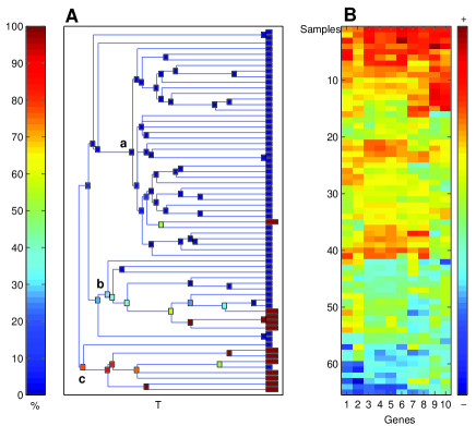
Refer to caption — Figure 1: $S1(G4)$ : clustering 65 tumors using the expression levels of gene cluster $G4$ . A. The boxes in the dendrogram represent clusters; they are colored according to their percentage of ER- tumors (see color bar on left). B. Clusters a,b,c are characterized, respectively, by high, intermediate and low expression levels (see color bar on right).

In the dendrogram Fig. 1A the boxes representing sample clusters were colored according to the percentage of ER- samples, ranging from red (100%) to blue (0%). In Fig. 1B the samples were ordered according to the dendrogram, and the colors represent the expression levels of the 10 genes. SPC generated 3 main branches (clusters); the upper - a with highest expression values, b - intermediate and the lowest - c. Cluster a, the biggest (41 samples), contains all but two of the tumors of the luminal-like (blue) cluster of PAL (see their Fig. 3). More interestingly, clusters a and b, contain 45 out of 48 of the ER+ tumors (see blue leaves). Cluster c is rich (7 out of 11) in ER- tumors. Designating any sample that does not belong to c as $ER+$ , we get our best classifier, with efficiency $E=45/48=0.94$ and purity $P=0.83$ . The corresponding numbers obtained by PAL (for their ”luminal-like” cluster) were $E=0.66$ and $P=0.89$ .

$S1(G30):$ $G30$ is a cluster of 15 genes, related to cell cycle proliferation. Only one of the 15 were included in PAL’s intrinsic set. Clustering the 65 tumors using the expression levels of these genes generated the dendrogram presented in Fig. 5A (see supplementary information). The boxes that represent sample clusters are colored according to their relative content of ER- samples. The dendrogram exhibits a clear partition of the tumors into clusters a with high expression levels of the $G30$ genes and c with intermediate expression levels, as seen in Fig. 5B. Cluster c contains 44 tumors, 38 of which were classified as ER+, 3 as ER- and 3 unknown. Hence this cluster captured the ER+ group with efficiency of $E=38/48=0.79$ and purity $P=38/44=0.86$ . Cluster a contains a high proportion of ER- tumors; its sub-cluster b consists of 5 special ER+ tumors that have relatively high expression levels of the $G30$ genes.

BREAST CANCER - SAL

Again we have two kinds of observations; those made using genes that were not included by SAL in their intrinsic set, and hence could not have been found by them, and observations made using genes that were included in the previous analysis.

Since there is considerable overlap between the samples of PAL and SAL, we did not repeat our attempt to reproduce all their findings. We did, however, study some aspects related to the clinical labels, that were the main additional feature of the SAL data. We emphasize here our findings concerning survival and p53 status. We found correlations between expression levels of several gene clusters and survival, and that the expression levels of these genes is also a predictor of p53 mutation status. We also present a very clear partition of the patients into two groups, for which we do not yet have any clinical interpretation.

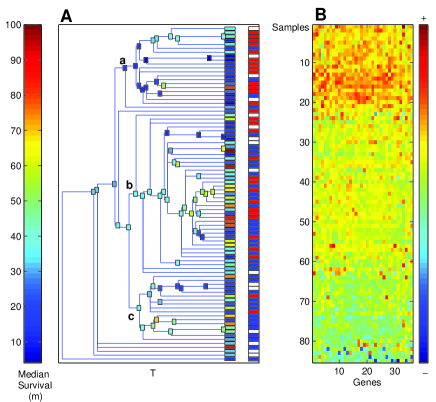
$S1(G10):$ cluster $G10$ contains 15 genes that are related to the ER pathway, including 5 of the 10 members of $G4$ mentioned in our analysis of PAL, (such as GATA-binding protein 3). Clustering the 85 samples ( $S1$ ) using $G10$ , generates the dendrogram presented in Fig. 6A (supplementary information). The boxes that represent sample clusters are colored according to the median value of the survival of the patients contained in each cluster, ranging from red (median survival of 100 months) to dark blue (4 months). Similarly to the results shown in Fig. 1, the variation in the expression levels of the $G10$ genes correlates well with the direct clinical measurements of the ER protein levels in the tumors. The dendrogram of Fig. 6A exhibits two main clusters; a contains most of the ER+ tumors, that exhibit higher expression levels of the $G10$ genes, as seen in Fig. 6B, and b, which contains mainly ER- tumors that exhibit low expression levels of the $G10$ genes.

Analyzing the correlation with the p53 status, wild type (wt) vs mutant, and with the survival parameter we get similar results as were obtained by SAL. They showed that the basal-like samples, corresponding to our cluster b, come from patients with the shortest survival times and a high frequency of p53 mutations. Two of the 17 members of cluster b survived for 41 months and all the others - for less than 26 months. The correlation coefficient between survival and the average expression levels of the $G10$ genes is 0.47. The Wilcoxon rank-sum test (WRST) indicated that to the distributions of survival times in cluster b to the rest of the patients are significantly different (P-value = $3.710^{-4}$ ); patients that exhibit low expression levels of the $G10$ genes have short survival.

To indicate the p53 status, we placed a color bar next to the leaves of the dendrogram, on which the patients with mutant p53 are labeled red and the p53 wt - blue. Patients with unknown p53 status were labeled white. Note that the 17 patients of cluster b exhibit low expression levels of the $G10$ genes. Ten of these 17 are p53 mutant, 5 have unknown labels and only two are wt. Hence low expression levels of the $G10$ genes seem to go along with a mutated p53. The correlation coefficient of the average expression levels of $G10$ with p53 status is 0.4; in particular, low expression is a good predictor of mutant p53. To substantiate the last statement, we compared the distributions (using WRST) of the median expression levels of patients with mutant p53 to wt. We found that the two distributions are significantly different (P-value= $1.210^{-4}$ ); the wt p53 patients exhibit high and the mutant p53 exhibit lower expression levels of the $G10$ genes.

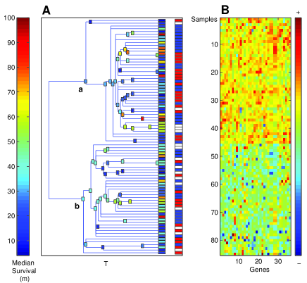
$S1(G33):$ Cluster $G33$ contains 36 genes, related to cell proliferation, which include 10 out of the 15 members of cluster $G30$ found by CTWC in our analysis of the PAL data. Clustering the 85 samples using the expression levels of these genes generated the dendrogram presented in Fig. 2A. The boxes are colored similarly to Fig. 6A; according to the median survival (in months), of the patients that belong to each cluster. The $G30$ genes partition the samples into 3 main clusters, a, b and c, as shown in the dendrogram. The corresponding $G33$ expression levels, as seen in Fig. 2B, are high, intermediate and low, respectively. The average expression level of the $G30$ genes is inversely correlated with survival (correlation coefficient -0.24). Cluster a contains patients with high expression and short survival; only one of its 21 members survived beyond 43 months, whereas clusters b and c contain long (up to 100 months) as well as short survival. Comparison of the distributions of the survival times of the patients in cluster a to those in clusters b and c indicates that there is a significant difference (P-value = 0.0016).

As to p53 status, we note that among the 21 patients in cluster a, 13 were mutant p53 and 4 had unknown status. Cluster c, of low expression levels, contains only two mutant p53 patients (out of 16 members of the cluster). The correlation coefficient between the average expression levels of $G33$ genes and p53 status is -0.4. Hence high expression levels of these genes is a good predictor for mutant p53, whereas low expression predicts wt p53. Comparison of the distributions of the median expression levels between the p53-mutant and the p53-wt patients yields significantly different distributions (P-value= $4.510^{-5}$ ).

$S1(G36):$ cluster $G36$ contains genes that are related to apoptosis suppression (e.g. bcl-2) and cell growth inhibition (e.g. INK4C cyclin-dependent kinase inhibitor 2c). Using the expression levels of this set of genes to cluster the 85 samples, we generate the dendrogram presented in Fig. 3A. The boxes are colored similarly to Fig. 2A, according to the median survival of the patients in each cluster. The dendrogram exhibits partition of the samples into two very distinct clusters; a contains patients with high expression levels and b - patients with low. We found no correlation between membership in either of these clusters and any of the clinical labels that were reported by SAL. However, the clarity of the partition calls for further investigation of the two groups of patients, which may reveal some so far unknown role played by the genes of $G36$ in breast cancer.

COLON CANCER

We applied CTWC on the colon data set of Notterman et al., containing 18 paired carcinoma and 4 paired adenoma samples. We refer to the set of all 44 samples as S and to the 36 paired carcinoma samples as S1. We present gene clusters which differentiate the samples according to the known normal/tumor classification, previously shown by Notterman et al.. Furthermore, we show the advantage of CTWC in mining new partitions which have not been found using other clustering methods and may contain relevant biological information.
Tumor - Normal separation

$S(G8):$ $G8$ contains 55 genes, which show high expression levels in the normal samples compared to the adenoma and carcinoma. Several genes within this cluster are known to be repressed in colorectal neoplasms; for example, guanilyn and DRA (down-regulated in adenoma). Some of these genes were previously mentioned by Notterman et al.Clustering the 44 samples, using the expression levels of $G8$ , generated the dendrogram shown in Fig. 4A.

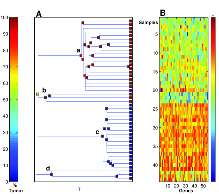
The dendrogram exhibits a clear separation into two large clusters (a and b) and two small ones (c and d). Clusters c and d contain all the normal samples (both carcinoma and adenoma), a - the tumor carcinoma samples and b - the tumor adenoma samples. The colors (see bar on the right hand side of the expression matrix - see reordered data) represent the expression levels of the genes in $G8$ , with red (blue) denoting high (low) values.

$S1(G25):$ The data set we analyzed next contains the 18 carcinoma and their paired normal samples, $S1$ . The group $G25$ contains 51 genes, some of which are known to be over expressed in carcinoma and are found to be related to colon cancer or other forms of neoplasma e.g, myc, matrilysin, GRO- $\gamma$ (see Notteman et al., 2001), and additional genes which may very well be related to colon cancer. Clustering the 36 samples of $S1$ , using the expression levels of the gene cluster $G25$ , gave rise to a clear partition of the samples into two clusters; one of normal samples (a), and the other of tumor samples (b), with relatively high expression levels of the $G25$ genes in the tumor cluster (see Fig. 7, supplementary information).
New observations (protocols A,B):
$S1(G3):$ Two experimental protocols that were used; 16 RNA samples (paired samples 3-6,8-10,11) were extracted using a method that isolates mRNA prior to reverse transcription (’protocol A’), and the other 20 samples (paired samples 12,27,28-29,32-35,39-40) were prepared by extracting total RNA from the cells (’protocol B’). Clustering the 36 carcinoma samples, using the expression levels of the 27 genes of cluster $G3$ , exhibits a clear partition of the samples into two clusters (see Fig 8A, supplementary information). Cluster b contains 20 tissues of protocol B, and cluster a contains 14 tissues of protocol A. This separation has two mistakes; both samples of patient 9 were labeled A and appear in the cluster of protocol B.
New observations (unknown interpretation):

$S10(G24),S10(G7),S10(G12):$ Clustering only the 18 carcinoma samples ( $S10$ , obtained in a previous CTWC iteration) on the basis of their expression over different sets of genes, revealed the following partitions:

The clustering operation $S10(G24)$ generated a clear separation of the tumor samples into 2 clusters. Samples 33,34,35,40 are clustered together in b, and show high expression levels of the $G24$ genes (Fig. 9, supplementary information).

The operation $S10(G7)$ separated tumor samples 27,32,33,40 from the other 14; the small group has low expression levels of the $G7$ genes (Fig. 10, supplementary information) .

$S10(G12)$ clustered tumor samples 33,34,35,12,40 together (cluster b in Fig. 11, supplementary information); the expression levels of the $G12$ genes are high in these 5 samples. Hence we discovered that tumor samples 33,40 and 35 were repeatedly separated from the remaining tumors, which implies that these patients may share some common characteristics, perhaps representing a true biological meaning. However, due to lack of additional information about the patients we were unable to determine the biological origin of this separation.

DISCUSSION AND CONCLUSION

We described the Coupled Two Way Clustering method and demonstrated it’s ability to extract useful information from breast cancer and colon cancer data. For both data sets we reproduced the findings of previous analyses and discovered new structure of biological significance, demonstrating the advantages of CTWC compared to standard clustering techniques.

The central strategy of CTWC is to cluster the samples on the basis of their expression levels over small, correlated sets of genes, and vice versa. The relevant sets of genes and samples are found by using, one at a time, stable clusters of genes (or samples), that were identified in preceding iterations of the algorithm. Whenever such a clustering operation generates new, statistically significant partitions of the clustered objects, the result is recorded, to be used in further iterations and to be scanned for possible biological or clinical interpretation.

Perou et al. also reached the conclusion that performing an ”all against all” analysis does not reveal the effects of relatively small groups of relevant genes. They were able to produce significant findings only after reduction of the genes used to a smaller number. The smaller ”intrinsic set” was identified using a particular guiding principle, one that can be used only when there are at least two samples from each of several patients. Furthermore, the selection criteria used exclude genes that, according to our findings, do contain important information.

CTWC does not only generate the important partitions of the samples; it also identifies small groups of genes that are responsible for the separation of different classes. For both breast and colon cancer we found partitions that have no clear interpretation at the moment, a fact that demonstrates the strength of unsupervised approaches such as clustering; unsuspected structure buried in the data can be revealed.

ACKNOWLEDGEMENTS

This research was partially supported by grants from the Germany - Israel Science Foundation (GIF), the Israel Academy of Sciences (ISF) and the Ridgefield Foundation. We thank D. Botstein for directing us to the two papers of the Stanford group on breast cancer (PAL and SAL).

REFERENCES

Alon,U., Barkai,N., Notterman,D.A., Gish,K., Ybarra,S., Mack,D. and Levine,A.J. (1999) Broad patterns of gene expression revealed by clustering analysis of tumor and normal colon tissues probed by oligonucleotide arrays, Proc. Natl. Acad. Sci. USA, 96, 6745–6750.

Blatt,M., Wiseman,S. and Domany,E. (1996) Superparamagnetic clustering of data, Phys. Rev. Lett., 76, 3251–3254.

Blatt,M., Wiseman,S. and Domany,E. (1997) Neural Comp. Data Clustering Using a Model Granular Magnet, 9, 1805–1842.

Califano,A., Stolovitsky,G. and Tu,Y. (2000) Analysis of Gene Expression Microarrays for Phenotype Classification, Proc. Int. Conf. Intell. Syst. Mol. Biol., 8, 75–85.

Cheng,Y. and Church,G.M. (2000) Biclustering of Expression Data, Proc. Int. Conf. Intell. Syst. Mol. Biol., 8, 93–103.

Domany,E., Blatt,M., Gdalyahu,Y. and Weinshall,D. (1999) Super-paramagnetic clustering of data: application to computer vision, Comp. Phys. Comm., 121–122.

Eisen,M.B., Spellman,P.T., Brown,P.O. and Botstein,D. (1998) Cluster analysis and display of genome-wide expression patterns, Proc. Natl. Acad. Sci. USA, 95, 14863–14868.

Fontemaggi,G., Kela,I., Amariglio, N., Rechavi, G., Krishnamurthy,J., Strano, S., Sacchi, A.,Givol, D. and Blandino, G. (2002) Identification of direct p73 target genes combining DNA microarray and chromatin immunoprecipitation analyses; Comparison with p53 targets, (unpublished).

Geisler,S., Lonning,P.E., Aas,T., Johnsen,H., Fluge,O., Haugen,D.F., Lillehaug,J.R., Akslen,L.A. and Borresen-Dale,A.L. (2001) Influence of TP53 gene alterations and c-erbB-2 expression on the response to treatment with doxorubicin in locally advanced breast cancer, Cancer Res., 6, 2505-2512.

Getz,G., Levine,E., Domany,E. and Zhang,M.Q. (2000) Super-paramagnetic clustering of yeast gene expression profiles, Physica A, 279, 457–464.

Getz,G., Levine,E. and Domany,E. (2000) Coupled two-way clustering analysis of gene microarray data, Proc. Natl. Acad. Sci. USA, 97, 12079–12084.

Getz,G. and Domany,E. (2002) Coupled Two-Way Clustering Server, (this issue).

Godard,S. et al,unpublished

Golub,T.R., Slonim,D.K., Tamayo,P., Huard,C., Gaasenbeek,M., Mesirov,J.P., Coller,H., Loh,M.L., Downing,J.R., Caligiuri,M.A., Bloomfield,C.D. and Lander,E.S. (1999) Molecular classification of cancer: class discovery and class prediction by gene expression monitoring., Science, 5439, 531-537.

Kannan,K., Amariglio,N., Rechavi,G., Jakob-Hirsch,J., Kela,I., Kaminski,N., Getz,G., Domany,E. and Givol,D. (2001) DNA microarrays identification of primary and secondary target genes regulated by p53, Oncogene, 20, 2225–2234.

Kela,I. (2002) Clustering of gene expression data. M.Sc. Thesis, Weizmann Institute (2002)

Notterman,D.A., Alon,U., Sierk,A.J. and Levine,A.J. (2001) Transcriptional gene expression profiles of colorectal adenoma, adenocarcinoma, and normal tissue examined by oligonucleotide arrays, Cancer Res. 7, 3124–3130.

Perou,C.M., Sorlie,T., Eisen,M.B., van de Rijn,M., Jeffrey,S.S., Rees,C.A., Pollack,J.R., Ross,D.T., Johnsen,H., Akslen,L.A., Fluge,O., Pergamenschikov,A., Williams,C., Zhu,S.X., Lonning,P.E., Borresen-Dale,A.L., Brown,P.O. and Botstein,D. (2000) Molecular portraits of human breast tumours, Nature, 406, 747–752.

Sorlie,T., Perou,C.M., Tibshirani,R., Aas,T., Geisler,S., Johnsen,H., Hastie,T., Eisen,M.B., van de Rijn,M., Jeffrey,S.S., Thorsen,T., Quist,H., Matese,J.C., Brown,P.O., Botstein,D., Eystein Lonning,P. and Borresen-Dale,A.L. (2001) Gene expression patterns of breast carcinomas distinguish tumor subclasses with clinical implications, Proc. Natl. Acad. Sci. USA, 19, 10869–10874.

Quintana,F., Getz,G., Hed,G., Domany,E., Cohen,I.R. (2002) Cluster analysis of human autoantibody reactivities in health and in type 1 diabetes mellitus: A bio-informatic approach to immune complexity, (unpublished).