Cluster Analysis of Gene Expression Data

Abstract

The expression levels of many thousands of genes can be measured simultaneously by DNA microarrays (chips). This novel experimental tool has revolutionized research in molecular biology and generated considerable excitement. A typical experiment uses a few tens of such chips, each dedicated to a single sample - such as tissue extracted from a particular tumor. The results of such an experiment contain several hundred thousand numbers, that come in the form of a table, of several thousand rows (one for each gene) and 50 - 100 columns (one for each sample). We developed a clustering methodology to mine such data. In this review I provide a very basic introduction to the subject, aimed at a physics audience with no prior knowledge of either gene expression or clustering methods. I explain what genes are, what is gene expression and how it is measured by DNA chips. Next I explain what is meant by ”clustering” and how we analyze the massive amounts of data from such experiments, and present results obtained from analysis of data obtained from colon cancer, brain tumors and breast cancer.

1 Reflection and Outline

The subject of this paper does not seem to have much to do with Statistical Mechanics, the subject I learned from Michael Fisher. Indeed the aim of the research I am describing is to gain understanding of Biology, and the methodology used is in the realm of Applied Mathematics and Pattern Recognition. Closer inspection reveals, however, that the ideas that underlie the approach rely strongly on the very subjects to which I have been introduced by Michael: Monte Carlo simulations[1] and phase transitions in Potts ferromagnets[2]. The problem area and technology I describe below are among of the most fascinating and exciting topics I encountered. I hope that Michael, who always had a keen interest in biology, will find the applicability of Statistical Physics to this type of research gratifying.

This paper has three parts, aimed at explaining the meaning of it’s title. The first part is a telegraphic introduction to the relevant biology, starting from genes and transcription and ending with an explanation of what DNA chips are and the kind of data that they produce. The second part is an equally concise introduction to cluster analysis, leading to a recently introduced method, Coupled Two-Way Clustering (CTWC), that was designed for the analysis and mining of data obtained by DNA chips. The third section puts the two introductory parts together and demonstrates how CTWC is used to obtain insights from the anaysis of gene expression data in several clinically relevant contexts, such as colon cancer, glioblastoma and breast cancer.

2 Introduction to the relevant biology

2.1 Genes and Gene Expression

Since my aim is to introduce only those concepts that are absolutely essential for understanding the data that will be presented and analyzed, I present here only a severely oversimplified description of a large number of very complex processes. The interested reader is referred to two excellent textbooks [3, 4].

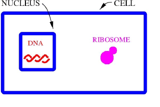
Figure 1: Caricature of a eucaryotic cell: its nucleus contains DNA, whereas the ribosomes are in the cytoplasm.

Cells and organisms are divided into two classes; procaryotic (such as bacteria) and eucaryotic. The latter have a nucleus; see the schematic drawing of Fig 1. The cell is enclosed by it’s membrane; embedded in the cell’s cytoplasm is it’s nucleus, surrounded and protected by its own membrane. The nucleus contains DNA, a one dimensional molecule, made of two complementary strands, coiled around each other as a double helix. Each strand consists of a backbone to which a linear sequence of bases is attached. There are four kinds of bases, denoted by C,G,A,T. The two strands contain complementary base sequences and are held together by hydrogen bonds that connect matching pairs of bases; G-C (three hydrogen bonds) and A-T (two).

A gene is a segment of DNA, which contains the formula for the chemical composition of one particular protein. Proteins are the working molecules of life; nearly every biological function is carried out by a protein. Topologically, a protein is also a chain; each link is an amino acid, with neighbors along the chain connected by covalent bonds. All proteins are made of 20 different amino acids - hence the chemical formula of a protein of length $N$ is an $N$-letter word, whose letters are taken from a 20-letter alphabet. A gene is nothing but an alphabetic cookbook recipe, listing the order in which the amino acids are to be strung when the corresponding protein is synthesized. Genetic information is encoded in the linear sequence in which the bases on the two strands are ordered along the DNA molecule. The genetic code is a universal translation table, with specific triplets of consecutive bases coding for every amino acid.

The genome is the collection of all the chemical formulae for the proteins that an organism needs and produces. The genome of a simple organism such as yeast contains about 7000 genes; the human genome has between 30,000 and 40,000. An overwhelming majority (98%) of human DNA contains non-coding regions (introns), i.e. strands that do not code for any particular protein.

Here is an amazing fact; every cell of a multicellular organism contains its entire genome! That is, every cell has the entire set of recipes the organism may ever need; the nucleus of each of the reader’s cells contains every piece of information needed to make a copy (clone) of him/her! Even though each cell contains the same set of genes, there is differentiation: cells of a complex organism, taken from different organs, have entirely different functions and the proteins that perform these functions are very different. Cells in our retina need photosensitive molecules, whereas our livers do not make much use of these. A gene is expressed in a cell when the protein it codes for is actually synthesized. In an average human cell about 10,000 genes are expressed.

The large majority of abundantly expressed genes are associated with common functions, such as metabolism, and hence are expressed in all cells. However, there will be differences between the expression profiles of different cells, and even in a single cell, expression will vary with time, in a manner dictated by external and internal signals that reflect the state of the organism and the cell itself.

Synthesis of proteins takes place at the ribosomes. These are enormous machines (made also of proteins) that read the chemical formulae written on the DNA and synthetise the proten according to the instructions. The ribosomes are in the cytoplasm, whereas the DNA is in the protected environment of the nucleus. This poses an immediate logistic problem - how does the information get transferred from the nucleus to the ribosome?

2.2 Transcription and Translation

The obvious solution of information transfer would be to rip out the piece of DNA that contains the gene that is to be expressed, and transport it to the cytoplasm. The engineering analogue of this strategy is the following. Imagine an architect, who has a single copy of a design for a building, stored on the hard disk of his PC. Now he has to transfer the blueprint to the construction site, in a different city. He probably will not opt for tearing out his hard disk and mailing it to the site, risking it being irreversibly lost or corrupted. Rather, he will prepare several diskettes, that contain copies of his design, and mail these in separate envelopes.

This is precisely the strategy adopted by cells.

         

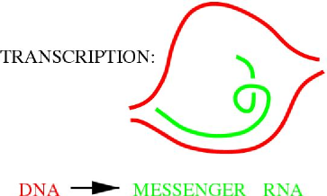
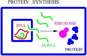
Figure 2: Transcription involves synthesis of mRNA, a copy of the gene encoded on the DNA (left). The mRNA molecules leave the nucleus and serve as the template for protein synthesis by the ribosomes (right).

When a gene receives a command to be expressed, the corresponding double helix of DNA opens, and a precise copy of the information, as written on one of the strands, is prepared (see Fig 2). This ”diskette” is a linear molecule called messenger RNA, mRNA and the process of its production is called transcription. The subsequent reading of the mRNA, deciphering the message (written using base triplets) into amino acids and synthesis of the corresponding protein at the ribosomes is called translation. In fact, when many molecules of a certain protein are needed, the cell produces many corresponding mRNAs, which are transferred through the nucleus’ membrane to the cytoplasm, and are ”read” by several ribosomes. Thus the single master copy of the instructions, contained in the DNA, generates many copies of the protein (see Fig 2). This transcription strategy is prudent and safe, preserving the precious master copy; at the same time it also serves as a remarkable amplifier of the genetic information.

A cell may need a large number of some proteins and a small number of others. That is, every gene may be expressed at a different level. The manner in which the instructions to start and stop transcription are given for a certain gene is governed by regulatory networks, which constitute one of the most intricate and fascinating subjects of current research. Transcription is regulated by special proteins, called transcription factors, which bind to specific locations on the DNA, upstream from the coding region. Their presence at the right site initiates or suppresses transcription.

This leads us to the basic paradigm of gene expression analysis:

The ”biological state” of a cell is reflected by its expression profile: the expression levels of all the genes of the genome. These, in turn, are reflected by the concentrations of the corresponding mRNA molecules.

This paradigm is by no means trivial or perfectly true. One may argue that the state of a cell at a given moment is defined by its chemical composition, i.e. the concentration of all the constituent proteins. There is no assurance that these concentrations are directly proportional to the concentrations of the related mRNA molecules. The rates of degradation of the different mRNA, the efficiency of their transcription to proteins, the rate of degradation of the proteins - all these may vary. Nevertheless, this is our working assumption; specifically, we assume that for human cells the expression levels of all 40,000 genes completely specify the state of the particular tissue from which the cells were taken. The question we turn to answer is - how does one measure, for a given cell or tissue, the expression levels of thousands of genes?

2.3 DNA chips

A DNA chip is the instrument that measures simultaneously the concentration of thousands of different mRNA molecules. It is also referred to as a DNA microarray (see [5] for a recent review of the technology, and the special supplement of Nature Genetics 21, Jan. 1999). DNA microarrays, produced by Affymetrix[6], can measure simultaneously the expression levels of up to 20,000 genes; the less expensive spotted arrays[7] do the same for several thousand. Schematically, the Affymetrix arrays are produced as follows. Divide a chip (a glass plate of about 1 cm across) into ”pixels” - each dedicated to one gene g. Billions of 25 base pair long pieces (oligonucleotides) of single strand DNA, copied from a particular segment of gene g are photolitigraphically synthesised on the dedicated pixel (these are referred to as ”probes”) . The mRNA molecules are extracted from the cells taken from the tissue of interest (such as tumor tissue obtained by surgery). They are Reverse Transcribed from RNA to DNA and their concentration is enhanced. Next, the resulting DNA is transcribed back into fluorescently marked single strand RNA. The solution of marked and enhanced mRNA molecules (”targets”) that are copies of the mRNA molecules that were originally extracted from the tissue, is placed on the chip and the labeled RNA are diffusing over the dense forest of single strand DNA probes. When such an mRNA encounters a part of the gene of which it is a perfect copy, it attaches to it - hybridizes - with a high affinity (considerably higher than with a bit of DNA of which it is not a perfect copy). When the mRNA solution is washed off, only those molecules that found their perfect match remain stuck to the chip. Now the chip is illuminated with a laser, and these stuck ”targets” fluoresce; by measuring the light intensity emanating from each pixel, one obtains a measure of the number of targets that stuck, which, in turn, is proportional to the concentration of these mRNA in the investigated tissue. In this manner one obtains, from a chip on which $N_{g}$ genes were placed, $N_{g}$ numbers that represent the expression levels of these genes in that tissue. A typical experiment provides the expression profiles of several tens of samples (say $N_{s}\approx 100$), over several thousand ($N_{g}$) genes. These results are summarized in an $N_{g}\times N_{s}$ expression table; each row corresponds to one particular gene and each column to a sample. Entry $E_{gs}$ of such an expression table stands for the expression level of gene $g$ in sample $s$. For example, the experiment on colon cancer, first reported by Alon et al [8], contains $N_{g}=2000$ genes whose expression levels passed some threshold, over $N_{s}=62$ samples, 40 of which were taken from tumor and 22 from normal colon tissue.

Such an expression table contains up to several hundred thousand numbers; the main issue addresed in this paper concerns the manner in which such vast amounts of data are ”mined”, to extract from it biologically relevant meaning. Several obvious aims of the data analysis are the following:

1. Identify genes whose expression levels reflect biological processes of interest (such as development of cancer).

2. Group the tumors ito classes that can be differentiated on the basis of their expression profiles, possibly in a way that can be interpreted in terms of clinical classification. If one can partition tumors, on the basis of their expression levels, into relevant classes (such as e.g. positive vs negative responders to a particular treatment), the classification obtained from expression analysis can be used as a diagnostic and thereupeutic tool.

3. Finally, the analysis can provide clues and guesses for the function of genes (proteins) of yet unknown role.

This concludes the brief and very oversimplified review of the biology background that is essential to understand the aims of this research. In what follows I present a method designed for mining such expression data.

3 Cluster Analysis

3.1 Supervised versus unsupervised analysis

Say we have two groups of samples, that have been labeled on the basis of some external (i.e. not contained in the expression table) information, such as clinical identification of tumor and normal samples; and our aim is to identify genes whose expression levels are significantly different for these two groups. Supervised analysis is the most suitable method for this kind of task. The simplest way is to treat the genes one at a time; for gene $g$ we have $N_{s}$ expression levels $A_{gs}$, and we propose as a null hypothesis that the these numbers were picked at random, from the same distribution, for all samples $s$. There are well established methods to test the validity of such a hypothesis and to calculate for each gene a statistic whose value indicates whether the null hypothesis should be accepted or rejected, as well as the probability $P_{g}$ for error (i.e. for rejecting the null hypothesis on the basis of the data, even though it is correct). An alternative supervised analysis uses a subset of the tissues of known clinical label to train a neural network to separate them into the known classes on the basis of their expression profiles. The generalization ability of the network is then estimated by classifying a test set of samples (whose correct labels are also known), that was not used in the training process.

The main disadvantage of supervised methods is their being limited to hypothesis testing. If one has some prior knowledge which can lead to a hypothesis, supervised methods will help to accept or reject it. They will never reveal the unexpected and never lead to new hypotheses, or to new partitions of the data. For example, if the tumors break into two unanticipated classes on the basis of their expression profiles, a supervised method will not be able to discover this. Another shortcoming is the (often very common) possibility of misclassification of some samples. A supervised method will not discover, in general, samples that were mistakenly labeled and used in, say, the training set.

The alternative is to use unsupervised methods of analysis. These aim at exploratory analysis of the data, introducing as little external knowledge or bias as possible, and ”let the data speak”. That is, we explore the structure of the data on the basis of correlations and similarities that are present in it. In the context of gene expression, such analysis has two obvious goals:

1. Find groups of genes that have correlated expression profiles. The members of such a group may take part in the same biological process.

2. Divide the tissues into groups with similar gene expression profiles. Tissues that belong to one group are expected to be in the same biological (e.g. clinical) state.

The method presented here to accomplish these aims is called clustering.

3.2 Clustering - statement of the problem.

The aims of cluster analysis [9, 10] can be stated as follows: given $N$ data points, $\mbox{\boldmath X}_{i},~{}~{}i=1,...,N$ embedded in $D$-dimensional space (i.e. each point is represented by $D$ components or coordinates), identify the underlying structure of the data. That is, peartition the $N$ points into $M$ clusters, such that points that belong to the same cluster are ”more similar” to each other than two points that belong to different clusters. In other words, one aims to determine whether the $N$ points form a single ”cloud”, or two, or more; in respectable unsupervised methods the number of clusters, $M$, is also determined by the algorithm.

The clustering problem, as stated above, is clearly ill posed. No definition was given for what is ”more similar”; furthermore, as we will see, the manner in which data points are assigned to clusters depends on the resolution at which the data are viewed. The last concern is addressed by generating a dendrogram or tree of clusters, whose number and composition varies with the resolution that is used. To clarify these points I present a simple example for a process of ”learning without a teacher”, of which clustering constitutes a particular case.

Imagine the following experiment; find a child who has never seen either a giraffe or a zebra, and expose him to a large number of pictures of these animals without saying a word of instruction. On each animal shown the child performs a series of $D$ measurements, two of which are most certainly $L$, the length of the neck, and $E$, the excentricity of the coloration (i.e. the ratio of the small dimension and the large). Each animal is represented, in the child’s brain, as a point in a $D$ dimensional space. Fig. 3 depicts the projection of these points on the two dimensional $(L,E)$ subspace.

         

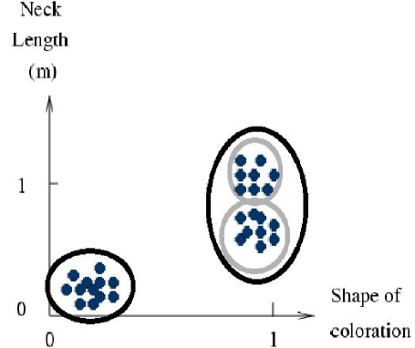
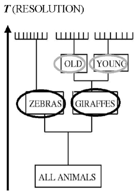
Figure 3: Left: Each zebra or giraffe is represented as a point on the neck length - coloration shape plane. The points form two clouds marked by the black ellipses. At higher resolution (controlled by the parameter $T$), we notice that the cloud of the giraffes is in fact composed of two slightly separated sub clouds. The corresponding dendrogram is presented on the right hand side.

Even though initially the child will see ”animals” - i.e. assign all points to a single cloud - with time he will realize (as his resolution improves) that in fact the data break into two clear clouds; one with small values of $L$ and $E$, corresponding to the zebras, and the second - the giraffes - with large $L$ and $E\approx 1$. The child, not having been instructed, will not know the names of the two kinds of animals he was exposed to, but I have no doubt that he will realize that two different kinds of creatures appear in the pictures. He has performed a clustering operation on the visual data he has been presented with.

Let us pause and consider the data and the statements that were made. Are there indeed two clouds in Fig 3? As we already said, when the data are seen with low resolution, they appear to belong to a single cloud of animals. Improved resolution leads to two clouds - and closer inspection reveals that in fact the cloud of giraffes breaks into two sub-clouds, of points that have similar colorations but different neck lengths! Apparently there were mature fully developed giraffes with long necks, and a group of young giraffes with shorter necks. Finally, when resolution is improved to the level of discerning individual differences between animals, each one forms his own cluster. Thus the proper way of representing the structure of the data is in the form of a dendrogram, also shown in Fig 3. The vertical axis corresponds to a parameter $T$ that represents the resolution at which the data are viewed. The horizontal axis is nominal - it presents a linear ordering of the individual data points (as identified by the final partition, in which each cluster consists of one individual point). The ordering is determined by the entire dendrogram - it can be thought of as a highly nonlinear mapping of the data from $D$ to one dimension. In any clustering algorithm that we use, we should look for the two features mentioned here, of (a) yielding a dendrogram that starts with a single cluster of $N$ points and ends with $N$ single-point clusters, and (b) providing a one-dimensional ordering of the data.

3.3 Clustering Algorithms

There are numerous clustering algorithms. Even though each aims at achieving a truly unsupervised and objective method, every one has built in, implicitly or explicitly, the bias of it’s inventor as to how a ”cluster should look” - e.g. a tight, spherical cloud, or a continuous region of high relative density and arbitrary shape, etc.

Average linkage [9], an agglomerative hierarchical algorithm that joins pairs of clusters on the basis of their proximity, is the most widely used for gene expression analysis [11]. K-means [9, 10] and Self Organized Maps [12] are algorithms that identify centroids or representatives for a preset number of groups; data points are assigned to clusters on the basis of their distances from the centroids. There are several physics related clustering algorithms, e.g. Deterministic Annealing [13] and Coupled Maps[14]. Deterministic Annealing uses the same cost function as K-means, but rather than minimizing it for a fixed value of clusters $K$, it performs a statistical mechanics type analysis, using a maximum entropy principle as its starting point. The resulting free energy is a complex function of the number of centroids and their locations, which are calculated by a minimization process. This minimization is done by lowering the temperature variable slowly and following minima that move and every now and then split (corresponding to a second order phase transition). Since it has been proven[15] that in the generic case the free energy function exhibits first order transitions, the deterministic annealing procedure is likely to follow one of it’s local minima.

We use another physics-motivated algorithm, which maps the clustering problem onto the statistical physics of granular ferromagnets [16].

3.4 SuperParamagnetic Clustering (SPC)

The algorithm [17] assigns a Potts spin $S_{i}$ to each data point $i$. We use $q=20$ components; the results depend very weakly on $q$. The distance matrix

$$D_{ij}=|\mbox{\boldmath X}_{i}-\mbox{\boldmath X}_{j}|$$ (1)

is constructed. For each spin we identify a set of neighbors; a pair of neighborings interact by a ferromagnetic[18] coupling $J_{ij}=f(D_{ij})$ with a decreasing function $f$. We used a Gaussian decay, but since the interaction between non-neighbors is set to $J=0$, the precise form of the function has little influence on the results.

The energy of a spin configuration $\{S\}$ is given by

$${\cal H}[\{S\}]=-\sum_{<ij>}J_{ij}[1-\delta(S_{i},S_{j})]$$ (2)

The summation runs over pairs of neighbors. We perform a Monte Carlo simulation of this disordered Potts ferromagnet at a series of temperatures. At each temperature $T$ we measure the spin-spin correlation for every pair of neighbors,

$$G_{ij}=<[\delta(S_{i},S_{j})-1/q]/[1-1/q]>$$ (3)

where the brackets $<\cdot>$ represent an equilibrium average of the ferromagnet (2), measured at $T$. If $i$ and $j$ belong to the same ordered ”grain”, we will have $G_{ij}\approx 1$, whereas if the two spins are uncorrelated, $G_{ij}\approx 0$. Hence we threshold the values of $G_{ij}$; if $G_{ij}>0.5$ the data points $i$ and $j$ are connected by an edge. The clusters obtained at temperature $T$ are the connected components of the resulting graph. In fact, the simple thresholding is supplemented by a ”directed growth” process, described elsewhere.

At $T=0$ the system is in its ground state, all $S_{i}$ have the same value, and this procedure generates a single cluster of all $N$ points. At $T=\infty$ we have $N$ independent spins, all pairs of points are uncorrelated and the procedure yields $N$ clusters, with a single point in each. Hence clearly $T$ controls the resolution at which the data are viewed; as it increases, we generate a dendrogram of clusters of decreasing sizes.

This algorithm has several attractive features, such as (i) the number of clusters is determined by the algorithm itself and not externally prescribed (ii) Stability against noise in the data; (iii) ability to identify a dense set of points, that form a cloud of an irregular, non-spherical shape, as a cluster. (iii) generating a hierarchy (dendrogram) and providing a mechanism to identify in it robust, stable clusters.

The physical basis for the last feature is that if a cluster is made of a dense set of points on a background of lower density, well separated from other dense regions, it will form (become an independent magnetized grain) at a low temperature $T_{1}$ and dissociate into subclusters at a high temperature $T_{2}$. The ratio of the temperatures at which a cluster ”dies” and ”is born”, $R=T_{2}/T_{1}$, is a measure of its stability.

SPC was used in a variety of contexts, ranging from computer vision [19] to speech recognition [17]. Its first direct application to gene expression data has been [20] for analysis of the temporal dependence of the expression levels in a synchronized yeast culture [21, 11], identifying gene clusters whose variation reflects the cell cycle. Subsequently, SPC was used [22] to identify primary targets of p53, a tumor suppressor that acts as a trascription factor of central importance in human cancer.

Our ability to identify stable (and statistically significant) clusters is of central importance for our usage of SPC in our algorithm for gene expression analysis.

4 Clustering Gene Expression Data

4.1 Two way clustering

The clustering methodology described above can be put to use for analysis of gene expression data in a fairly straightforward way, bearing in mind the questions and aims metioned above.

We clearly have two main seemingly distinct aims; to identify groups of co-regulated genes which probably belong to the same machinery or network, and to identify molecular characteristics of different clinical states and discriminators between them. The obvious way to go about these two tasks is by Two Way Clustering. First view the $N$ samples as the objects to be clustered; each is represented by a point in a $G$ dimensional ”feature space”, where $G$ is the number of genes for which expression levels were measured (in fact one works only with a subset of the genes on a chip - those that pass some preset filters). This analysis yields a dendrogram of samples, with each cluster containing samples with sizeable pairwise similarities of their expression profiles measured over the entire set of genes.

The second way of looking at the same data is by considering the genes as the objects to be clustered; $G$ data points embedded in an $N$ dimensional feature space. This analysis groups together genes on the basis of their correlations over the full set of samples. In Fig. 4 we present the results of two-way clustering data obtained for 36 brain tumors (see th enext section for details). We show here the expression matrix, with the rows corresponding to the genes and columns to samples. The dendrograms the correspond to the two clustering operations described above are shown next to the matrix, whose rows and columns have been already permuted according to the linear order imposed by the two dendrograms.

This is the type of analysis that has been widely used in the gene expression clustering literature. It represents a holistic approach to the problem; using every piece of reliable information to look at the entire grand picture. This apprach does have, however, several obvious shortcomings; overcoming these was the motivation to develop a method which can be viewed as taking a more reductioninst approach, while improving significantly the signal to noise ratio of the processed data.

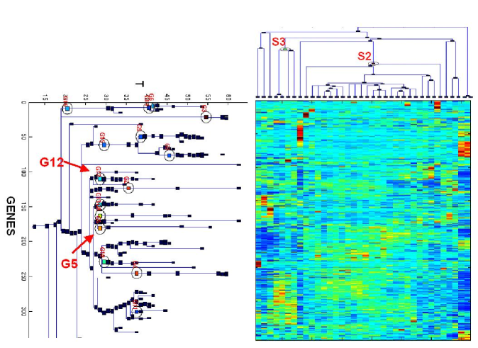
Figure 4: Two-way clustering of brain tumor data; the two dendrograms, of genes and samples, are shown next to the expression matrix.

4.2 Coupled Two Way Clustering - Motivation

The main motivation of introducing CTWC [23] was to increase the signal to noise ratio of the expression data. There are two different kinds of ”noise” the method is designed to overcome.

The first of these is a problem generated by the very advantage and most exciting aspect of DNA-chips - the ability to view expression levels of a very large number of genes simultaneously. Say one stays, after initial filtering, with two thousand genes, and one wishes to study a particular aspect of the samples (e.g. differentiating between several kinds of cancer). Chances are that the genes which participate in the pathology of interest constitute only a small subset of the total 2000 - say we have 40 genes whose expression indeed distinguishes the samples on the basis of the process that is studied. Hence the desired ”signal” resides in 2 % of the total genes that are analysed; the remaining 98 % behave in a way that is uncorrelated with these and introduce nothing but noise. The contribution of the relevant genes to the distance between a pair of samples will be overwhelmed by the random signal of the much larger irrelevant set. My favorite example for this situation is that of a football stadium, in which 99,000 spectators scream at random, while 1000 others are singing a coherent tune. These 1000 are, however, scattered all over the stadium - the chance that a listener, standing at the center of the field, will be able to identify the tune are very small. If only we could identify the singers, concentrate them into one stand and point a directional microphone at them - we could hear the signal!

In the language of gene expression analysis, we would like to identify the relevant subset of 40 genes, and use only their expression levels to characterize the samples. In other words, to project the datapints representing the samples from the 2000 dimensional space in which they are embeddded, down to a 40 dimensional subspace, and to assess the structure of the data (e.g. - do they form two or more distinct groups?) on the basis of this projected representation. A similar effect may arise due to the subjects; a partition of the genes which is much more relevant to our aims could have been obtained had we used only a subset of the samples.

Both these examples have to do with reducing the size of the feature space. Sometimes it is important to use the reduced set of features to cluster only a subset of the objects. For example, when we have expression profiles from to kinds of leukemia patients, ALL and AML, with the ALL patients breaking further into two sub-families, of T-ALL and B-ALL, the separation of the latter two subclouds of points may be masked by the interpolating presence of the AML group. In other words, a special set of genes will reveal an internal structure of the ALL cloud only when the AML cloud is removed [23].

These two statements amount to a need to work with special submatrices of the full expression matrix. The number of such submatrices is, however, exponential in the size of the dataset, and the obvious question that arises is - how can one select the ”right” submatrices in an unsupervised and yet efficient way? The CTWC algorithm provides a heuristic answer to this question.

4.3 Coupled Two Way Clustering - Implementation

CTWC is an iterative process, whose starting point is the standard two way clustering mentioned above. Denote the set of all samples by S1 and that of all genes used as G1. The notation S1(G1) stands for the clustering operation of all samples, using all genes, and G1(S1) for clustering the genes using all samples. From both clustering operations we identify stable clusters of genes and samples, i.e. those for which the stability index $R$ exceeds a critical value and whose size is not too small. Stable gene clusters are denoted as GI with I=2,3,… and stable sample clusters as SJ, J=2,3,… In the next iteration we use every gene cluster GI (including I=1) as the feature set, to characterize and cluster every sample set SJ. These operations are denoted by SJ(GI) (we clearly leave out S1(G1)). In effect, we use every stable gen cluster as a possible ”relevant gene set”; the submatrices defined by SJ and GI are the ones we study. Similarly, all the clustering operations of the form GI(SJ) are also carried out. In all clustering operations we check for the emergence of partitions into stable clusters, of genes and samples. If we obtain a new stable cluster, we add it to our list and record its members, as well as the clustering operation that gave rise to it. If a certain clustering operation did not give rise to new significant partitions, we move down the list of gene and sample clusters to the next pair.

This heuristic identification of relevant gene sets and submatrices is nothing but an exhaustive search among the stable clusters that were generated. The number of these, emerging from G1(S1) is a few tens, whereas S1(G1) generates a few stable sample clusters usually. Hence the next stage typically involves less than a hundred clustering operations. These iterative steps stop when no new stable clusters beyond a preset minimal size are generated, which usually happens after the first or second level of the process.

In a typical analysis we generate between 10 and 100 interesting partitions, which are searched for biologically or clinically interesting findings, on the basis of the genes that gave rise to the partition and on the basis of available clinical labels of the samples. It is important to note that these labels are used a posteriori, after the clustering has taken place, to interpret and evaluate the results.

5 Applications of CTWC for gene expression data analysis

So far CTWC has been applied primarily to analysis of data from various kinds of cancer. In some cases we used publicly available data, with no prior contact with the groups that did the original acquisition and analysis. Our initial work on colon cancer [8] and leukemia [24] fall in this category.

Subsequently we collaborated with a group at the University Hospital at Lausanne (CHUV) on Glioblastoma - in this work we were involved from early in the data acquisition stage. Our current collaborations include work on colon cancer and breast cancer. In the latter case we worked with publicly available data, but its choice and the challenge to improve on existing analysis came from a biologist. We are also involved in work on leukemia and on meiosis [25] in yeast; finally, the same method was applied successfully [26] to analyze data obtained from an ”antigen chip”, used to study the antibody repertoire of subjects that suffer from autoimmune diseases, such as diabetes.

I will limit the discussion here to presentation a few select results obtained for glioblastoma [27] and for breast cancer [29].

5.1 CTWC analysis of brain tumors (gliomas)

Brain tumors are classified into three main groups. Low grade astrocytoma (A) are small sized tumors at an early stage of development. Cancerous growth may recur after their removal, giving rise to secondary gliomas (SC). The third kind are primary (PR) glioblastoma (GBM); this classification is assigned when at the stage of initial diagnosis and discovery the tumor is already of a large size. A dataset $S1$ of 36 samples was obtained by a group from the University Hospital at Lausanne [27]. 17 of these were from PR GBM, 4 - from SC, 12 were from A and 3 from human glioma cell lines grown in culture. Expression profiles were obtained using Clontech Atlas 1.2 arrays of 1176 genes. For each gene $g$ the measured expression value for tumor sample $s$ was divided by its value in a reference sample composed of a mixture of normal brain tissue. We filtered the genes by keeping only those for which the maximal value of this ratio (over the 36 samples) exceeded its minimal value by at least a factor of two. 358 genes passed this filter and constituted our full gene set $G1$, which was clustered using expression ratios over $S1$. The $G1(S1)$ clustering operation (see Fig 4) yielded 15 stable gene clusters. The complementary operation $S1(G1)$ did not yield any partition of the samples that could be given clear clinical interpretation.

One of the stable gene clusters, $G5$, contained 9 genes. When the expression levels of only these genes are used to characterize the tumors [in the operation denoted $S1(G5)$], a large and stable cluster, $S11$, of 21 tumors, emerged (see Fig 5.

Figure 5: The operation $S1(G5)$, clustering all tumors on the basis of their expression profiles over the genes of cluster $G5$. A stable cluster, $S11$ emerges, containing all the non-primary tumors and only two of the primaries.

This cluster contained all the 12 astrocytoma and all 4 SC tumors. Three of the remaining 5 tumors of $S11$ were cell lines and two were registered as PR GBMs. Pathological diagnosis was redone for these two tumors; one was found to contain a significant oligoastrocytoma component, and much of the piece of the other, that was used for RNA extraction, was diagnosed as of normal brain ifiltrative zone. Hence the expression levels of $G5$ gave rise to a nearly perfect separation of PR from non-PR (A and SC tumors). The genes of $G5$ were significantly upregulated in PR and downregulated in A and SC.

These findings made good biological sense, since three of the genes in $G5$ (VEGF, VEGFR and PTN) are related to angiogenesis. Angiogenesis is the process of development of blood vessels, which are essential for growth of tumors beyond a certain critical size, bringing nutrition to and removing waste from the growing tissue. Upregulation of genes that are known to be involved in angiogenesis is a logical consequence of the fact that PR GBM are large tumors.

An important application of the method concerns investigation of the genes that belong to $G5$; in particular, one of the genes of $G5$, IGFBP2, was of considerable interest with little existing clues to its function and role in cancer development. Our finding, that its expression is strongly correlated with the angiogenesis related genes came as a surprise that was worth detailed further study. The co-expression of genes from the IGFBP family with VEGF and VEGFR has been demonstrated in an independent experiment that tested this directly for cell lines under different conditions.

This example demonstrates the power of CTWC; a subgroup of genes with correlated expression levels was found to be able to separate PR from non-PR GBM, whereas using all the genes introduced noise that wiped out this separation. In addition, by looking at the genes of this correlated set, we provided an indication for the role that a gene with previously unknown function may play in the evolution of tumors.

For other findings of interest in this data set we refer the reader to the paper by Godard et al [27].

5.2 Breast Cancer Data

In a different study, on breast cancer, we used publicly available expression data of Perou et al [28]. The choice of this particular data set was guided by D. Botstein, who informed us that these were of the highest quality, were submitted to most extensive effort for analysis and challenged us to demonstrate that our method can extract findings that eluded previous treatments. The results of this study are available[29]; here I present only one particular new finding.

The Stanford data contained expression profiles of 65 human samples ($S1$) and 19 cell lines. 40 tumors were paired, with samples taken before and after chemotherapy (with doxorubicin), to which 3 (out of 20) subjects responded positively. 1753 genes ($G1$) passed initial filtering; the clustering operation $S1(G1)$, of all the samples using their expression profiles over all these genes, did not yield any clear meaningful partitions. Perou et al realized the same point that has motivated us to construct CTWC, namely that one has to prune the number of genes that are used in order to improve the signal to noise ratio. They ranked the genes according to a figure of merit they introduced, which measures the proximity of expressions of the two samples taken from the same patient before and after chemotherapy, versus the (expectedly larger) dissimilarity of samples from different patients. The 496 top scorers constituted their ”intrinsic gene set” which was then used to cluster the samples.

We did not use this intrinsic set but rather, applied CTWC on the full sets of samples and genes. In the $G1(S1)$ operation we found several stable gene clusters. One of these, $G46$, contained 33 genes, whose expression levels correlate well with the cells’ proliferation rates. Only 2 out of these made it into the intrinsic set of Perou et al; hence they could not have found any result that we obtained on the basis of these genes.

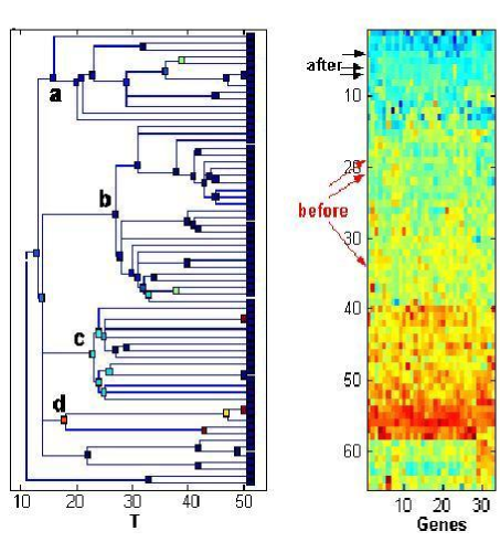
Figure 6: The operation $S1(G46)$, clustering all tumors on the basis of the proliferation related genes of $G46$. We found a cluster (b) which contained all three samples from patients for who chemotherapy was successful, taken before the treatment. Cluster (b) contained 10 out of the 20 ”before” samples.

The operation $S1(G46)$ identified three main clusters; (a) of samples with low proliferation rates - these are ’normal breast - like’; (b) samples with intermediate, and (c) with high proliferation rates. Interestingly, the ”before treatment” samples taken from all three tumors for which chemotherapy did succeed were in cluster (b), whereas the corresponding ’after treatment’ samples were in (a), the ’normal breast - like’ cluster. Therefore the genes of $G46$ can perhaps be used a posteriori, to indicate success of treatment on the basis of their expression measured after treatment and, more importantly, may have predictive power with respect to the probability of success of the doxorubicin therapy. that was used. Intermediate expression of the G46 genes may serve as a marker for a relatively high success rate of the Doxorubicin treatment (3/10 versus 3/20 for the entire set of ”before treatment” samples). Clearly these statements are backed only by statistics based on small samples, but they do indicate possible clinical applications of the method, provided experiments on more samples strengthen the statistical reliability of these preliminary findings.

6 Summary

DNA chips provide a new, previously unavailable glimpse into the manner in which the expression levels of thousands of genes vary as a function of time, tissue type and clinical state. Coupled Two Way Clustering provides a powerful tool to mine large scale expression data by identifying groups of correlated (and possibly co-regulated) genes which, in turn, are used to divide the samples into biologically and clinically relevant groups. The basic ”engine” used by CTWC is a clustering algorithm rooted in the methodology of and insight gained from Statistical Physics.

The extracted information may enlarge our body of general basic knowledge and understanding, especially of gene rgulatory networks and processes. In addition, it may provide clues about the function of genes and their role in various pathologies; one can also hope to develop powerful diagnostic and prognostic tools based on gene microarrays.

References

- [1] E. Domany, K.K. Mon, G.V. Chester and M. E. Fisher, Phys. Rev. B 12, 5025 (1975).
- [2] D. Mukamel, M. E. Fisher and E. Domany, Phys. Rev. Lett. 37, 565 (1976).
- [3] B. Alberts, D. Bray, J. Lewis, M. Raff, K. Roberts and J. D. Watson, Molecular iology of the Cell, 3rd edition, (Garland Publishing, New York, 1994).
- [4] J. L. Gould and W. T. Keeton, Biological Science, 6th edition (W.W. Norton & Co., New York, London, 1996).
- [5] A. Schulze and J. Downward, Nature Cell. Biol. 3,190 (2001)
- [6] See http://www.affymetrix.com for information.
- [7] See http://cmgm.stanford.edu/pbrown/mguide/index.html
- [8] U. Alon, N. Barkai, D.A. Notterman, K. Gish, S. Ybarra, D. Mack, and A.J. Levine Proc. Natl Acad. Sci. USA 96,6745 (1999).
- [9] A. K. Jain and R. C. Dubes, Algorithms for Clustering Data, (Prentice Hall, Englewood Cliffs NJ, 1988).
- [10] O.R. Duda, P. E. Hart and D. G. Stork, Pattern Classification (John Wiley & Sons Inc., New York 2001)
- [11] M. Eisen, P. Spellman, P. Brown, and D. Botstein, Proc. Natl. Acad. Sci. USA 95, 14863 (1998).
- [12] T. Kohonen, Self Organizing Maps (Springer, Berlin, 1997).
- [13] K. Rose, E. Gurewitz and G. C. Fox, Phys. Rev. Lett. 65, 945 (1990).
- [14] L. Angelini, F. De Carlo, C. Marangi, M. Pellicor and S. Stramaglia, Phys. Rev. Lett 85, 554 (2000).
- [15] J. Schneider, Phys. Rev. E 57, 2449 (1998)
- [16] M. Blatt, S. Wiseman, and E. Domany Phys. Rev. Lett. 76, 3251 (1996).
- [17] M. Blatt, S. Wiseman, and E. Domany Neural Comp.9, 1805 (1997).
- [18] Non-ferromagnetic Potts models can be obtained from maximum likelihood and maximum entropy principles; see M. Blatt, Ph. D. Thesis, Weizmann Inst. Of Science (1997) and L. Giada and M. Marsili, Phys. Rev. E 63, 1101 (2001).
- [19] E. Domany, M. Blatt, Y. Gdalyahu and D. Weinshall, Comp.Phys.Comm. 121, 5 (1999).
- [20] G. Getz, E. Levine, E. Domany, and M. Zhang Physica A 279, 457 (2000).
- [21] P. T. Spellman et al, Mol.Biol.Cell 9, 3273 (1998).
- [22] K. Kannan, N. Amariglio, G. Rechavi, J. Jakob-Hirsch, I. Kela, N. Kaminski, G. Getz, E. Domany and D. Givol, Oncogene 20, 2225 (2001).
- [23] G. Getz, E. Levine and E. Domany, Proc. Natl. Acad. Sci. USA 97, 12079 (2000).
- [24] T.R. Golub, D.K. Slonim, P. Tamayo, C. Huard, M. Gaasenbeek, J.P. Mesirov, H. Coller, M.L. Loh, J.R. Downing, M.A. Caligiuri, C.D. Bloomfield, and E.S. Lander Science 286, 531 (1999).
- [25] M. Primig et al, Nature Genetics 26, 415 (2000).
- [26] F. Quintana, G. Getz, G. Hed, E. Domany and I. R. Cohen, (submitted 2002).
- [27] S. Godard, G. Getz, H. Kobayashi, M. Nozaki, A.-C. Diserens, M.-F. Hamou, R. Stupp, R. C. Janzer, P. Bucher, N. de Tribolet, E. Domany, M. E. Hegi,(submitted, 2002).
- [28] C.M. Perou et al Nature 406, 747 (2000).
- [29] I. Kela, Unraveling Biological Information from Gene Expression Data, Using Advanced Clustering Techniques(M.Sc. Thesis, Weizmann Institute of Science, 2001).