Process Pathway Inference
via Time Series Analysis

Abstract

Motivated by recent experimental developments in functional genomics, we construct and test a numerical technique for inferring process pathways, in which one process calls another process, from time series data. We validate using a case in which data are readily available and formulate an extension, appropriate for genetic regulatory networks, which exploits Bayesian inference and in which the present–day undersampling is compensated for by prior understanding of genetic regulation.

Preprint number: NSF-ITP-02-47

1 Motivation

The last decade has witnessed stunning advances in experimental biology, particularly in the fields of neuroscience and genomics, which have made possible ‘data–driven’ biological investigations. As examples, the quantitative revolution of genomics has provided terabytes of transcriptome data; and neuroscientists routinely record for hours or even days from multiple neurons simultaneously. This transformation stands as a challenge to theorists who hope to advance understanding by making connection between experiment and first principles models.

In genomics, for example, we are presented with the expression levels of thousands of genes, but our ability to model is limited not only quantitatively, in that there are myriad unknown rate constants and binding parameters, but qualitatively, in that a sizable fraction of proteins and genes remain of uncharacterized function [1]. Similarly, in neuroscience, we can model patches of cellular membranes, synapses, and (at least electro–physiologically) entire cells [2]. However, this modeling hinges on numerous unknown parameters, and even if we can perform massive computations involved in the study of even rather small biological neural networks, the sensitivity to these parameters still makes the whole approach intractable. The astronomical amounts of experimental data are troubling computationally, but even more immediate problems are the lack of reductive descriptions of the underlying phenomena and undersampling — an inability of the data to determine the (slightly smaller) astronomical number of important microscopic parameters appearing in theoretical models.

Presented with such an imbalance, it is important to distinguish among the possible questions we can ask as well as the possible tools at our disposal for answering them. That is, one can ask what the system is doing (a nontrivial question when the language for discovery is an astronomical number of unorganized data) before one asks how it is doing what it does. The latter involves building models of some microscopic fidelity. The former may be answered without reference to microscopics by a model–independent, data–driven phenomenological approach.

A useful historical analogy is that of particle physics of the late 1950’s, in which an explosion of data from accelerators was equally daunting and similarly irreducible. At that time physicists were not yet asking the how questions (cross sections, isospin multiplets, etc.) but were instead carefully, statistically, inferring the presence or absence of features in the data; for example, exploiting prior knowledge of quantum mechanics to constrain reasonable shapes for peaks in the data (hallmarks of newly discovered particles — the ‘resonances’).

In this analogy, neuroscience is still dealing with the existence of peaks. Indeed, only recently (see Ref. [3] and further works by the same authors) it has become clear that precise timings of single spikes are very important for understanding the neural code. This is a basic, objective, model–independent observation, and it is not surprising that Shannon’s information theory, which was specifically designed with these types of questions in mind, turned out to be extremely useful.

In genomics, however, the quantities of interest are easier to identify: gene expressions are largely governed by the underlying regulation networks. Now is the time to attempt to infer these networks — still the what question — which corresponds to inferring the peaks in the data. This is a requisite step before classifying the possible networks and explaining the classification rules — an answer to how the system does what it does. Trying to answer how before carefully exploring what might ultimately produce many epi–manipulations of the data, but little significant understanding.

Said otherwise, presented with data describing natural phenomena, one should form a phenomenology of experimental results, then inferences from the data in light of this phenomenology, and finally microscopic models. Genomics is currently at the penultimate step, and, armed with careful informatics, here meaning the incorporation of data with prior knowledge in the absence of detailed models, we hope to reduce the data into a representation which allows description, prediction, and ultimately control.

An example of data reduction convenient for representation is cataloging of the regulatory networks. However, such cataloging is not a model independent task: at the very least, our microscopic model includes the existence of the networks. Further, even if we are only interested in a network’s connection diagram and do not care much about the exact details of the connections, identification of the network still involves determination of many parameters. Thus it is not clear that information–theoretic approaches will be of great use. However, it is plausible that our intuition of how the underlying microscopic dynamics translates into macroscopic probabilistic models may play a big role. The main purpose of this paper is to show that this intuition, appropriately mathematized in a principled way as the a priori knowledge — the priors in Bayesian statistics — may be self–consistently incorporated into a macroscopic probabilistic model of process pathways without detailed, sophisticated modeling of microscopic dynamics. We will first show this on a simple synthetic example, and then suggest some extensions of the ideas with an eye towards genetic regulatory networks.

2 Functional genomics

As mentioned, the motivating problem here is time series informatics applied to functional genomics. We therefore briefly review genetics and characterize the relevant experiments, the data from which will be used in inferring the underlying connectivities and possibly control.

2.1 A brief review of genetics

The central goal of functional genomics is the understanding of the interactions among distinct parts of the genome — the genes. Each gene consists of long words composed of thousands of coding base pairs of DNA which are then transcribed into mRNA, which is then translated into protein. Many of these proteins, called transcription factors, then regulate the rate of production of mRNA transcribed either by their own genes or other genes. The working of all the genes thus forms a genetic regulatory network, and may be thought of as a dynamical system. Inputs include elements of the physical world which affect the activity of the transcription factors, and outputs may be considered as the concentrations of the translated proteins or, at a deeper level, the transcribed mRNA. While the proteins are ultimately responsible for cellular function, the mRNA are more easily experimentally measured via DNA microarrays.

2.2 A brief review of DNA microarrays

Only recently has it become possible to probe the expression of a number of genes comparable to the total number of genes in the entire genome of an organism via microarrays of nucleic acids, commonly known as ‘DNA chips.’ The most common application of such a chip is to monitor simultaneously the expression of thousands of genes by detecting hybridization of nucleic acid originating from a biological sample to target nucleic acids lying on the chip. One can then probe, for example, the differences in gene expression between cancerous and non–cancerous cells of the same specialization [4, 5, 6, 7, 8, 9, 10], or the expression of different genes as a function of the phase of the cell cycle [11, 12], or of the response of cells to chemical or physical perturbation. The two latter types of experiments produce time series of gene expressions, and they will be the focal point of our discussion from now on.

The first DNA microarrays were made by Affymetrix in the early 1990s [13, 14, 15]. In this technique, DNA oligonucleotides are attached to a surface in a specific spatial pattern, directed by optically activated chemical synthesis. One can build an arbitrary oligonucleotide sequence in a small area (approximately 20 microns per target) on the surface. However, the initial setup cost of creating the chip makes the technique infeasible for any application for which less than several hundred masks will be created (and sold). Individual researchers are completely without flexibility to change the chip to fit a particular area of investigation.

Functional genomics further benefited from a second technology in 1996, when Pat Brown’s lab at Stanford introduced the spot chip [16, 17]. This highly customizable technique exploits robotic deposition of drops on a microscope slide. The automation makes creating new and different slides a simple operation. Moreover, one can create typically 120 slides at a time. Individual researchers can thus design custom experiments, placing genes at locations or redundancies of their choosing. The gene fragments used in the spotting technique are hundreds of base pairs in length, and therefore less sensitive to single base pair mismatches.

3 Methods

3.1 Chemical network reconstruction

Genomic data is certainly not the first dynamic data for which reverse engineering of the interaction network has been attempted. A similar problem has been faced historically in chemistry, in which one would like to infer the underlying reactions responsible for observed data. Such reaction networks typically are sparse, that is, the typical connectivity is far less than the total number of chemical species. This is also true in genomics, where one gene typically interacts with no more than a few dozen others [18].

To highlight the parallels, one may state the question as follows: armed with sufficient temporal data taken from a number of interacting reagents (here, chemicals), is it possible to infer the circuit diagram? One possible strategy was proposed in 1995 [19], tested first on simulated data, and later on the glycolytic pathway [20], and recently refined in light of ideas from information theory [21]. However, this strategy has yet to be successfully applied to any reactions which were not known by the authors beforehand, nor subjected to a ‘blind’ test, as in the annual CASP test among the protein folding community. In addition, unlike in chemical kinetics, where the data is produced by moderately nonlinear and rapidly interrogated dynamical systems, genomic datasets are highly undersampled and are more like a set of fuzzy logic gates, or leaky boolean circuits. Thus, successful application of techniques inspired by chemical networks to genomic data is, at best, doubtful.

We may nonetheless attempt reverse engineering of regulatory networks with a similar philosophy, in that, rather than trying to fit to a precise microscopic model, we attempt to parameterize a minimal phenomenological model and infer macroscopic parameters from it.

3.2 Synthetic network reconstruction

In order to test any new attempt to infer connectivity from dynamics, it is useful to study a system which is qualitatively similar, e.g., which demonstrates degrees of freedom which turn on and off other degrees of freedom in a near–complete or ‘fuzzy logic gate’ way and for which connectivity is sparse; yet for which data are readily available and obvious to interpret. To that end, we collected data from a multiuser UNIX machine, recording the relative CPU usage of all processes (the analogue of mRNA concentration), user ID, and process name, as a function of time. This can be done in an automated way via bash script, and the results analyzed via MATLAB.

A typical time course, automatically labeled via MATLAB, is shown in Fig. 1 for a particular (anonymous) user at a large department of applied mathematics.

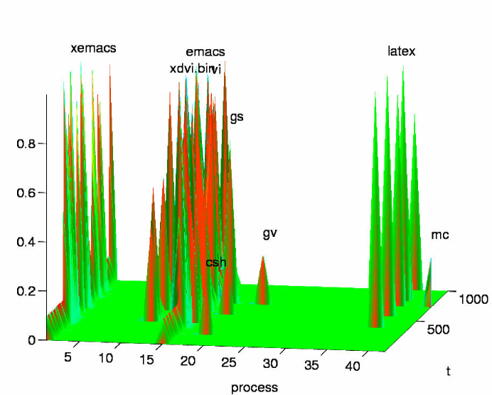
Figure 1: CPU percentage for all the processes called by a particular user during the observation (approximately $10^{3}$ seconds). Processes are numbered according to their relative frequency over all users during the observation time.

One axis is the job ‘number,’ ordered by frequency of occurrence over all users; the other axis is time (roughly in seconds). The height (and color) indicates CPU usage.

3.3 Modeling synthetic data

We begin with the minimal probabilistic model of process pathways, in which the strength of each process at subsequent time steps is linearly determined by the strength of all current processes. Similar linear models have been used with some success in understanding genomic data, including clustering via dynamics [22]. The most general model in discrete time is the $AR(p)$ model, in which we include the possibility that the state now is a function of the $p$ previous observations of the system. We do not yet include the possibility of hidden degrees of freedom. Mathematically, we may pose the model as

$${\mathbf{g}}_{t} = {\mathbf{w}}_{0}+{\mathbb{M}}_{1}{\mathbf{g}}_{t-1}+{\mathbb{M}}_{2}{\mathbf{g}}_{t-2}+\ldots+{\mathbb{M}}_{p}{\mathbf{g}}_{t-p}+\boldsymbol{\xi}_{t}$$ (1)

$$\langle\xi_{i,t}\xi_{j,t^{\prime}}\rangle = C^{ij}\delta_{t,t^{\prime}},$$ (2)

where the degree of freedom at observation $t$ is ${\mathbf{g}}_{t}$, the transition matrices are ${\mathbb{M}}_{j}$, and the noise correlation ${\mathbb{C}}$ is as–yet undetermined.

One may fit for the most probable transition matrices ${\mathbb{M}}_{j}$ as well as the offset ${\mathbf{w}}_{0}$ and the noise correlation matrix ${\mathbb{C}}$, using, for example, the standard Schwartz’s Bayesian Information Criterion [23] to determine the most likely value of $p$. Excellent numerical techniques and general purpose libraries have been designed for solving this problem [24].

Note that we do not claim the actual interactions among the processes are linear, as Eq. (1) seems to imply. Indeed, as stated above, the exact values of the transition matrices ${\mathbb{M}}_{j}$ are of very little interest to us, and we are only interested in the topological features of the network. It is reasonable to expect that the absence of a connection between two processes will be fit well by a zero in the corresponding transition matrix element, while the presence of a connection of any type will result in its nonzero value. The mismatch between the linear form of Eq. (1) and the actual dynamics will manifest itself in a large variance $C^{ij}$. However, if we are not interested in the exact values of ${\mathbb{M}}_{j}$, this should not adversely effect our determination of connections.

4 Results

Fitting the observed CPU usages to the transition state model, one finds the most probable $p$ value is $1$, indicating a lack of inertia in the system; the resulting transition matrix ${\mathbb{M}}_{1}$ is plotted in Fig. 2. The noise covariance matrix was quite small, despite the naiveté of the model.

Figure 2: The transition state matrix ${\mathbb{M}}_{1}$ resulting from the data in Fig. 1.

Causal connections between jobs are labeled with ‘$\rightarrow$’, e.g., ‘emacs$\rightarrow$latex’ or ‘emacs drives latex.’ We highlight several remarkable features:

1. Processes familiar to anyone who has used the typesetting software LaTeXwill be readily apparent: one edits a file (e.g., in emacs, xemacs, or vi), then compiles with latex, and views the result in xdvi and finally ghostscript (‘gs’). Similarly one observes emacs drives latex, latex drives gs, etc.

2. Note that the matrix is not symmetric: one axis describes processes which ‘activate’ other processes; the second describes which process is acted on. For example, latex drives ghostscript but ghostscript does not drive latex.

3. The transition matrix shows ‘upregulation’ as well as ‘downregulation’: some processes discourage other processes at later times.

4. Diagonal elements have not been labeled as they simply describe the likelihood the process will continue on to the next time step.

5. Note also how the transition matrix correctly infers the highly sparse connectivity of these disparate jobs. The vast majority of elements are $0$, as they should be, since processes are not influenced by those called by other users.

For comparison, in Fig. 3 we also show an example of a transition matrix when the CPU usages are replaced with randomly generated data. Any reasonable structure is absent here. These results are in accord with our intuition that the proposed probabilistic model for data reduction, Eq. (1), although an incomplete description, still leads to a reasonable reconstruction of network connectivity.

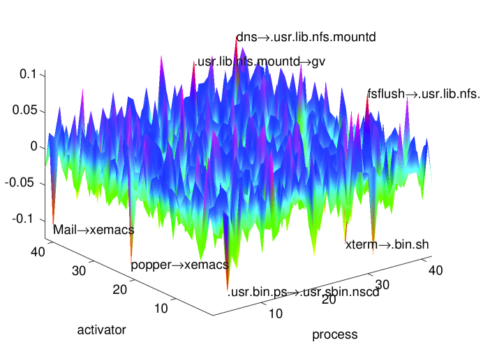
Figure 3: The transition state matrix ${\mathbb{M}}_{1}$ resulting from random data.

5 Modeling gene regulation

In the example above, as mentioned, data are plentiful. In genomic time series, data are scarce. However, the above exercise is designed to test a phenomenological model into which one can incorporate additional knowledge about genetic regulation. This goal, constraining possible models by compensating for sparse data with prior knowledge, is mathematized via Bayesian analysis.

We emphasize that we are not using Bayesian analysis to attempt to fit for the innumerable unknowns in a microscopic model, e.g., a chemical kinetics model of transcriptional regulation. We are not interested in these parameters but in couplings and network topology. We instead augment the successful phenomenological or ‘macroscopic’ model above with prior knowledge about transcriptional regulation.

5.1 Bayesian statistics

A brief summary of Bayesian statistics is in order. We refer the interested reader to standard textbooks (cf. Ref. [25]) for discussions of philosophical implications of Bayesian statistics, as well as standard statistical properties of Bayesian estimators. We focus below only on the relevant features.

Bayes rule itself,

$$P(b|a)=\frac{P(a|b)P(b)}{P(a)}\;,$$ (3)

is merely a rewriting of the rules of joint probabilities. The connection with interpretation of experiments is made by identifying $b$ as the model, or specifically the vector of parameters ${\boldsymbol{\theta}}$ of the model; and $a$ as the data $D$. Then

$$P({\boldsymbol{\theta}}|D)=\frac{P(D|{\boldsymbol{\theta}})P({\boldsymbol{\theta}})}{P(D)}\;,$$ (4)

$$P(D)=\int d{\boldsymbol{\theta}}\,P({\boldsymbol{\theta}},D)=\int d{\boldsymbol{\theta}}\,P(D|{\boldsymbol{\theta}})P({\boldsymbol{\theta}}).$$ (5)

In Eq. (4), the left hand side is called the posterior, and the first term in the numerator in the right hand side is called the likelihood. The strength of Bayesian methods comes from $P({\boldsymbol{\theta}})$, the prior. The prior summarizes knowledge about the probability of a model before the the results, $D$, of an experiment are observed. When experimental data are abundant the exact specification of the prior is usually unimportant (cf. Refs. [26, 27]); when data are scarce the prior constrains the space of available models. While careless a priori assumptions may constrain the observer to the wrong part of the model space, in the analysis of genetic regulatory networks one may exploit well established knowledge about transcriptional regulation to construct appropriate priors, as we illustrate in Sec. 5.2.2.

Armed with the prior, one next finds the a posteriori expected value of the parameters:

$$\langle{\boldsymbol{\theta}}\rangle_{D}=\int d{\boldsymbol{\theta}}\,{\boldsymbol{\theta}}P({\boldsymbol{\theta}}|D)=\frac{\int d{\boldsymbol{\theta}}\,{\boldsymbol{\theta}}\,P({\boldsymbol{\theta}})P(D|{\boldsymbol{\theta}})}{P(D)}\equiv\frac{\langle{\boldsymbol{\theta}}\,P(D|{\boldsymbol{\theta}})\rangle}{\langle P(D|{\boldsymbol{\theta}})\rangle}\;,$$ (6)

where $\langle\dots\rangle$ and $\langle\dots\rangle_{D}$ denote expectations over the prior and the posterior respectively. When the number of data $N$ is large we expect the posterior to be tightly peaked around some value $\widehat{{\boldsymbol{\theta}}}$ which maximizes the posterior (maximum a posteriori probability, or MAP, values), and then $\widehat{{\boldsymbol{\theta}}}$ is the first order term in the saddle point asymptotic expansion of $\langle{\boldsymbol{\theta}}\rangle_{D}$ in powers of $1/N$.

Even for severely undersampled problems, $N$ is usually large enough so that $\widehat{{\boldsymbol{\theta}}}\approx\langle{\boldsymbol{\theta}}\rangle_{D}$, and it is tempting to replace integrals in Eq. (6) by their saddle point values. One of the greatest realizations in Bayesian theory in the last decades was that such replacement is wrong [23, 28, 26, 29, 30]. Indeed, when averaging over all possible models, each of the integrals in Eq. (6) will have a contribution from fluctuations around the value $\widehat{{\boldsymbol{\theta}}}$. For example, under some very general conditions, and with an assumption that $\log P(D|{\boldsymbol{\theta}})$ scales linearly in the number of data, the total probability of the data, $P(D)$, has the following expansion in powers of $1/N$

$$\log P(D)=\log P(D|\widehat{{\boldsymbol{\theta}}})-\frac{K}{2}\log N-\frac{1}{2}\log\det\left[\left.\frac{\partial^{2}}{\partial\theta_{i}\partial\theta_{j}}\right|_{\widehat{{\boldsymbol{\theta}}}}\frac{\log P(D|{\boldsymbol{\theta}})}{N}\right]+\log P(\widehat{{\boldsymbol{\theta}}})+o(N^{0})\;,$$ (7)

where $K$ is the number of parameters in the model (dimensionality of ${\boldsymbol{\theta}}$). The integral in the numerator of Eq. (6) can be written in a similar fashion. We see that the terms beyond the maximum likelihood contribution $\log P(D|\widehat{{\boldsymbol{\theta}}})$ are generally negative and their magnitude grows with $K$. Thus these terms provide a built–in punishment for model complexity. For this reason, they are known in the literature as as the Occam razor (cf. Ref. [30]).

To illustrate, imagine that the prior admits two model families $\Theta^{1}$ and $\Theta^{2}$ with different parameters ${\boldsymbol{\theta}}^{1}$, ${\boldsymbol{\theta}}^{2}$, such that $K_{1}\equiv\dim{\boldsymbol{\theta}}^{1}<K_{2}\equiv\dim{\boldsymbol{\theta}}^{2}$. As an example, consider fitting a function with a polynomial of low degree ($K_{1}$) or high degree ($K_{2}$). Usually we would expect the model family with more parameters to be better at explaining the data: $P(D|\widehat{{\boldsymbol{\theta}}^{2}})>P(D|\widehat{{\boldsymbol{\theta}}^{1}}).$ Thus if we were to choose a model family that explains the data best based on the maximum likelihood alone, a more complex model would win. However, the estimates within the larger model family, $\Theta^{2}$, are less robust to small fluctuations, and this is picked up by the integration over all parameters: even though $P(D|\widehat{{\boldsymbol{\theta}}^{1}})$ may be smaller than $P(D|\widehat{{\boldsymbol{\theta}}^{2}})$, the relation between the probabilities of the model families $P(\Theta^{1}|D)$ and $P(\Theta^{2}|D)$, as determined by Eqs. (6, 7), may be different. In particular, for $N\gg 1$ the likelihood term, which scales linearly with $N$, always wins, and Bayesian model selection approaches that of the maximum likelihood. However, for small $N$ the difference between the likelihood and the other terms in Eq. (7) is less profound, and a simpler model family, which is not the best in explaining the data, may turn out victorious.

In short, Bayes rule shows how a simpler model may be less likely, yet more probable.

Before ending our quick review of Bayesian statistics, two more comments are in order. First, as the model selection arguments are mostly important for small $N$, where $\log N\sim 1$, it would be a mistake to ignore $O(1)$ terms in Eq. (7) and use just $K/2\log N$ as a model complexity punishment (Schwartz’s Bayesian Information Criterion [23], also mentioned in Sec. 3.3). In particular, we believe that such replacement may be a cause of a common observation that the Bayesian Criterion overpunishes complex models (cf. Ref. [31]). Second, even though in this work we will be mostly dealing with finite parameter models, application of nonparameteric methods to biological data certainly holds promise. Occam–type arguments for such cases have been discussed in, for example, Refs. [32, 27].

5.2 Bayesian inference of regulatory dynamics

5.2.1 A simple model

Let ${\mathbf{g}}_{t}$ stand for the vector of expressions (mRNA concentrations) of genes in a microarray experiment at time $t$. The number of genes, $K_{\mathbf{g}}\equiv\dim{\mathbf{g}}_{t}$, can be on the order of thousands. In principle, ${\mathbf{g}}_{t+1}$ can depend on concentrations at all times that preceded $t+1$. However, if we view the gene expression mechanism in cells as a realization of some chemical kinetics, governed by first order differential equations, then it is reasonable to expect that the concentrations depend only on their immediate past, i.e., ${\mathbf{g}}_{t+1}={\mathbf{f}}({\mathbf{g}}_{t})$. We begin with the simplest possible dynamic, a simplified version of Eqs. (1, 2):

$${\mathbf{g}}_{t+1}-{\mathbf{g}}_{t} = {\mathbb{M}}{\mathbf{g}}_{t}+\boldsymbol{\xi}_{t}\;,$$ (8)

$$\langle\xi_{i,t}\xi_{j,t^{\prime}}\rangle = \sigma^{2}\,\delta_{ij}\delta_{t,t^{\prime}}\;,$$ (9)

where the noise is Gaussian, and ${\mathbb{M}}$ and $\sigma$ are unknown. This is equivalent to

$$P({\mathbf{g}}_{t+1}|{\mathbf{g}}_{t},{\mathbb{M}},\sigma)=\frac{1}{\left(2\pi\sigma^{2}\right)^{K_{\mathbf{g}}/2}}\exp\left[-\frac{1}{2\sigma^{2}}\big{\langle}\big{|}{\mathbf{g}}_{t+1}-{\mathbf{g}}_{t}-{\mathbb{M}}{\mathbf{g}}_{t}\big{|}^{2}\big{\rangle}_{t}\right]\;.$$ (10)

where $\langle\cdots\rangle_{t}$ indicates empirical averaging over time.

Notice that unlike in Eqs. (1, 2) the noise in this model is not correlated among the genes; moreover, variances are equal for all genes. Below we formulate an extension that incorporates hidden degrees of freedom (e.g., biochemistry) whose omission may otherwise lead to large or correlated noise (cf. Sec. 5.2.3). However, with only a handful of experiments available we cannot hope that data will be able to determine millions of elements of a full covariance matrix. As data become more plentiful, it may even make sense to bypass Eqs. (8, 9) completely and pursue model independent feature extraction (as formulated in Secs. 6.1 and 6.2). Below we pursue the possibility that the current simple model exhibits some of the success evidenced in Sec. 4.

5.2.2 Biological priors

Even in the simplistic form of Eqs. (8, 9), the dynamic still contains too many parameters ($\sim K_{\mathbf{g}}^{2}$) to be tractable. We therefore search for biologically motivated priors to constrain the possible values of ${\mathbb{M}}$. An example of such a prior would be, for example, that genes with similar regulatory sequences should be regulated similarly. More directly, genes whose promoters have similar numbers of certain important motifs should be co–expressed, an ansatz used with notable success by Bussemaker et al. [34] in discovering regulatory regions.

This may be expressed in the following prior

$$P({\mathbb{M}}|\mu,\ell)\propto\exp\left[-\frac{\ell^{2}}{2}\sum_{i\neq j,k}^{K_{\mathbf{g}}}\left(\frac{M_{ik}-M_{jk}}{d_{ij}}\right)^{2}-\frac{\mu^{2}}{2}\sum_{ij}^{K_{\mathbf{g}}}M_{ij}^{2}\right]\;,$$ (11)

where the first term punishes for different regulation of genes with similar regulating sequences, and the second assures proper normalization of priors by effectively constraining the range of possible $M_{ij}$. Here $d_{ij}$ is a distance function measuring deviation between regulatory regions of genes $i$ and $j$ in terms of the number of each regulatory motif appearing, weighted by the relative importance of that motif, found by considering the entire time series as in Ref. [34] or ‘quality factors’ as in Ref. [35].

The parameter $\ell$ plays the role of a smoothing length, as in Ref. [32], and, lacking a first–principles estimate of its value, we must integrate over $\ell$, weighted by an appropriate prior. As explained in Ref. [27], it is not only likely that such integration will choose the proper value of $\ell$ almost independently of such prior, but it may even balance a slightly improper choice of the distance measure $d_{ij}$ and the difference form $(M_{ik}-M_{jk})^{2}$. The same comments relate to the mass $\mu$ and the noise variance $\sigma$ as well.

An enjoyable feature of this prior is that, like the likelihood, Eq. (10), it is exponentially quadratic in the unknowns ${\mathbb{M}}$. Thus the posterior expectations are Gaussian integrals, which may be performed analytically using the standard Wigner current technique [36]. Following Eq. (6) we find for the a posteriori values of the connection matrix:

$$\left<M_{ij}\right>_{D} = \left.\frac{\partial}{\partial J_{ij}}\right|_{{\mathbb{J}}=0}\log Z({\mathbb{J}})\;,$$ (12)

$$Z({\mathbb{J}}) = \int d\sigma\,d\mu\,d\ell P(\sigma)P(\mu)P(\ell)\left[\frac{\det\mathbf{\cal A}}{\det(\mathbf{\cal A}+\mathbf{\cal G})}\right]^{1/2}$$ (13)

$$\times\exp\left[\frac{1}{2}\left({\mathbb{B}}+{\mathbb{J}}\right)(\mathbf{\cal A}+\mathbf{\cal G})^{-1}\left({\mathbb{B}}+{\mathbb{J}}\right)\right]\;.$$

Here the curvature tensor $\mathbf{\cal A}$ at the saddle point of Eq. (11) is given by

$$A_{ij,kl} = \left[{\mu^{2}}+\ell^{2}\sum_{m}^{K_{\mathbf{g}}}\left(c_{mj}+c_{mi}\right)\right]\delta_{ik}\delta_{jl}-2\ell^{2}c_{ik}\delta_{jl}\,$$ (14)

and the time–lagged correlation, equal–time correlation, and ‘closeness’ (the inverse of the distance matrix) matrices are

$${\mathbb{B}} = \frac{1}{\sigma^{2}}\left<({\mathbf{g}}_{t+1}-{\mathbf{g}}_{t}){\mathbf{g}}_{t}^{T}\right>_{t}$$ (15)

$${\mathbb{G}} = \frac{1}{\sigma^{2}}\left<{\mathbf{g}}_{t}{\mathbf{g}}_{t}^{T}\right>_{t}\;,\;\;\;\;\mathbf{\cal G}={\mathbb{I}}\otimes{\mathbb{G}}\;,$$ (16)

$$c_{ij} = \begin{cases}d_{ij}^{-2}&\text{if $i\neq j$},\\ 0&\text{if $i=j$}.\end{cases}$$ (17)

The mass $\mu$ regulates the integrals and is expected to be small. Then $\det\mathbf{\cal A}/\det(\mathbf{\cal A}+\mathbf{\cal G})$ scales as a large positive power of $\ell^{2}/(\ell^{2}+{\rm const})$, and therefore decreases as $\ell$ decreases. On the other hand, the exponent in Eq. (13) involves $(\mathbf{\cal A}+\mathbf{\cal G})^{-1}$, which scales as $1/(\ell^{2}+{\rm const})$ for large $\ell$. The exponent thus decreases as $\ell$ increases. We may then reasonably expect that the integrand in Eq. (13) will be peaked at some non–trivial value of $\ell$; this peak should be sharp since both ${\mathbb{B}}$ and $\mathbf{\cal G}$ involve large number of samples. This may be viewed as the smoothing length selection by the data [27].

Note that the priors over the hyperparameters $\sigma,\mu,\ell$ in Eq. (13) are as yet undefined. Since, as mentioned above (see also Refs. [26]), their actual forms are of little importance, we may hope that by choosing them appropriately we may be able to render the integrals in Eq. (13) analytically tractable.

5.2.3 Hidden control

The formalism deserves experimental testing. However, one further extension offers a substantial improvement. DNA microarrays offer only a partial view into the workings of a cell, since numerous important degrees of freedom remain unobserved. In mathematical modeling of the yeast cell cycle, for example, considerable effort has been exerted to fine–tune models in which only chemistry controls the processes, and the genetic expression is a mere passive function of this chemical control. While this may or may not prove to be an accurate characterization, some chemical control unobserved by gene chip experiments certainly exists. Inclusion will clearly necessitate a model of some structure other than that of Eq. (8). Unlike the assumption of linearity, which merely leads to misestimation of the values of interactions, this effect may make the dynamical system appear to be not of first order, or introduce a gene–dependent noise correlation matrix and artificial couplings between genes that dominate the real ones. To avoid this, we need to supplement the vector of genes ${\mathbf{g}}$ with a vector of unknown hidden degrees of freedom ${\mathbf{h}}$. Then the evolution will take form

$$\begin{pmatrix}{\mathbf{g}}_{t+1}-{\mathbf{g}}_{t}\\ {\mathbf{h}}_{t+1}-{\mathbf{h}}_{t}\end{pmatrix} = \begin{pmatrix}{\mathbb{M}}^{\rm gg}&{\mathbb{M}}^{\rm gh}\\ {\mathbb{M}}^{\rm hg}&{\mathbb{M}}^{\rm hh}\end{pmatrix}\begin{pmatrix}{\mathbf{g}}_{t}\\ {\mathbf{h}}_{t}\end{pmatrix}+\begin{pmatrix}\boldsymbol{\xi}_{t}\\ \boldsymbol{\eta}_{t}\end{pmatrix}\;,$$ (18)

$$\langle\xi_{i,t}\xi_{j,t^{\prime}}\rangle = \sigma^{2}\,\delta_{ij}\delta_{t,t^{\prime}}\;,$$ (19)

$$\langle\eta_{t}^{i}\eta_{t^{\prime}}^{j}\rangle = \,v_{ij}\delta_{t,t^{\prime}}\;.$$ (20)

Within Bayesian analysis, one may integrate over the unknown degrees of freedom and their possible couplings while remaining agnostic about the identities of ${\mathbf{h}}$, and similarly sum over their possible dimensionality $K_{\mathbf{h}}$. As data are scarce, it is reasonable to expect that models with small number of hidden units will dominate the posterior. Thus we allow a full correlation matrix for the Gaussian noise in the hidden units, $\boldsymbol{\eta}_{t}$, since this adds only a few additional parameters to our model (${\mathbb{M}}^{\rm gg}$, of course, has a few million), but allows necessary flexibility.

One will need a prior over newly introduced ${\mathbb{M}}$’s. Since chemistry couples to expression via the transcription factors, and therefore via the regulatory sequences, we can write a similar prior as above, namely

$$P({\mathbb{M}}^{\rm gh}|\mu_{\rm gh},\ell)\propto\exp\left[-\frac{\ell^{2}}{2}\sum_{i\neq j}^{K_{\mathbf{g}}}\sum_{k}^{K_{\mathbf{h}}}\left(\frac{M^{\rm gh}_{ik}-M^{\rm gh}_{jk}}{d_{ij}}\right)^{2}-\frac{\mu_{\rm gh}^{2}}{2}\sum_{i}^{K_{\mathbf{g}}}\sum_{j}^{K_{\mathbf{h}}}(M^{\rm gh}_{ij})^{2}\right]\;,$$ (21)

with a different mass, but the same kinetic term as in Eq. (11). In the absence of precise identification of the hidden degrees of freedom, we lack a biological prior on ${\mathbb{M}}^{\rm hg},{\mathbb{M}}^{\rm hh}$ and must therefore choose a prior that does not spoil the analytic tractability of the resulting integrals.

6 Outlook

The main difficulty in obtaining time series data is not biological or technological, but rather financial. Affymetrix chips, the more reliable of the two dominant technologies, are quite expensive. As estimated in [38], a 24-point time series with replication factor of 3 currently costs $\sim\$57,600$. As the cost of the technology decreases, and as data become more plentiful, the role of priors in inferring connectivity and possible causation diminishes.

Moreover, as noted before, with increasing data comes the possibility of model independent, nonparametric feature extraction by learning the joint probability distributions of expression levels at different times (cf. Ref. [32]). We highlight two promising such directions below.

6.1 Mutual information and entropy distance

A completely model independent visualization tool of informatics is a low dimensional embedding of the connectivity diagram of the multiple genes via some meaningful metric. To this end, armed with a successfully learned joint probability, one may use information theory to define distance in a principled way.

An example of such a diagram based on information theoretic ideas is presented for simulated chemical kinetics in [21], in which the mutual information

$$I(i\rightarrow j) = \int dg_{i}dg^{+}_{j}P(g_{i},g^{+}_{j})\log_{2}\left(\frac{P(g_{i},g^{+}_{j})}{P(g_{i})P(g_{j})}\right)$$ (22)

was used for embedding, with the time–lagged joint probability of degrees of freedom $P(g_{i},g_{j}^{+})\equiv\langle P(g_{i}(t),g_{j}(t+\tau))\rangle_{t}$ learned by histogramming. While mutual information is a useful similarity measure, it is not a distance in that it does not obey the triangle inequality. However, the ‘entropy distance’

$$D_{H}(i\rightarrow j)=-\int dg_{i}dg^{+}_{j}P(g_{i},g^{+}_{j})\log_{2}\left(\frac{P(g_{i},g^{+}_{j})^{2}\sigma_{i}\sigma_{j}}{P(g_{i})P(g_{j})}\right)$$ (23)

does obey the triangle inequality [39] and thus can be used as a metric, based on which one can form an embedding in lower dimensions and construct a process diagram as in Refs. [19, 20, 21]. Here, by $\sigma_{\{i,j\}}$ we mean the uncertainties in measurements of $g_{\{i,j\}}$, respectively. Note that this distance is reparameterization invariant under monotonic reparameterizations $x\rightarrow f(x);y\rightarrow g(y)$, $\sigma_{x}\rightarrow\sigma_{f}/f^{\prime}$, etc.

6.2 Clustering by meaningful information: the information bottleneck

Clustering without identifying a specific property of interest is meaningless. In most cases, if we try to learn from data (fit a curve, select a model, extrapolate, cluster, etc.) we are doing so not to find the parameters per se, but to use them to make predictions of future data [40]. Thus in dynamics the variables of relevance are the future gene expressions, and one should cluster data by maximally compressing them while retaining the most information about the subsequent time steps.

This idea was put on firm information–theoretic ground recently with the development of the information bottleneck [41], which, given a joint probability distribution between degrees of freedom (e.g., gene expressions at some time) and a quantity of interest (e.g., gene expressions at subsequent times), allows an iterative calculation of the meaningful clusters in a probabilistic clustering algorithm.

An important aspect omitted from current formulations of the information bottleneck is Bayesian integration over possible joint probability distributions; this procedure smoothes the data and avoids clustering noise. We expect that this will be one of the most promising as well as principled lines of research in bioinformatics.

6.3 Prognosis

The future is promising for such data–driven techniques: data are becoming more plentiful, computational power continues to exponentiate, and the data themselves are becoming more reliable, as those who hope to interpret them study more carefully their statistics and analyses. However, before any new techniques in computational biology will be widely exploited, they must be ‘verified’ by comparing with results agreed upon in the biological community. In this case, verification will entail corroboration of inferred causal relations among genes (or within an inferred module of genes) with the biological literature. We anticipate that such time series based techniques will find common usage as tests for consensus with known connectivities become more standardized, and we look forward to their continued development and implementation.

Acknowledgments

The authors are grateful to Dimitris Anastassiou, Guillaume Bal, William Bialek, Harmen Bussemaker, Michael Elowitz, Stanlslas Leibler, Christina Leslie, Bud Mishra, Alex Rikun, Burkhard Rost, Ana Radovanovic, Andrey Rzhetsky, Misha Samoilov, Tapio Schneider, Boris Schraiman, Susanne Still, Naftali Tishby, and John Tyson for many stimulating discussions. The authors were partially supported by NSF Grant No. PHY–9907949 to the Kavli Institute for Theoretical Physics.

References

- [1] G. D. Stormo and K. Tan. Mining genome databases to identify and understand new gene regulatory systems. Current Opinion in Microbiology, 5:149–153, 2002.
- [2] P. Dayan and L. F. Abbott. Theoretical Neuroscience: Computational and Mathematical Modeling of Neural Systems. MIT Press, Cambridge, MA, 2001.
- [3] F. Rieke, D. Warland, R. de Ruyter van Steveninck, and W. Bialek. Spikes: Exploring the Neural Code. MIT Press, Cambridge, MA, 1996.
- [4] M. G. Walker, W. Volkmuth, E. Sprinzak, D. Hodsdon, and T. Kliner. Prediction of gene function by genome–scale expression analysis: Prostate cancer–associated genes. Genome Research, 9:1198–1203, 1999.
- [5] T. R. Golub et al. Molecular classification of cancer: class discover and class prediction by gene expression monitoring. Science, 286:628–629, 1999.
- [6] U. Alon. Broad pattern of gene expression revealed by clustering analysis of tumor and normal colon tissues probed by oligonucleotide arrays. PNAS USA, 96:6745–6750, 1999.
- [7] C. M. Perou et al. Distinctive gene expression patterns in human mammary epithelial cells and breast cancers. PNAS USA, 96:9212–9217, 1999.
- [8] D. T. Ross et al. Systematic variation in gene expression patterns in human cancer cell lines. Nature Genetics, 24:227–235, 2000.
- [9] U. Scherf et al. A gene expression database for the molecular pharmacology of cancer. Nature Genetics, 24:236–244, 2000.
- [10] D. Pinkel. Cancer cells, chemotherapy, and gene clusters. Nature Genetics, 24:208–209, 2000.
- [11] R. Cho et al. A genome–wide transcriptional analysis of the mitotic cell cycle. Mol. Cell, 2:65–71, 1998.
- [12] P. T. Spellman et al. Comprehensive identification of cell cycle–regulated genes of the yeast saccharomyces cerecisiae by microarray hybridization. Mol. Biol. Cell, 9:3273–3297, 1998.
- [13] S. P. A. Fodor, J. L. Read, M. C. Pirrund, L. Styer, A. T. Lu, and D. Solas. Light-directed, spatially addressable parallel chemical synthesis. Science, 251:767–773, 1991.
- [14] S. P. A. Fodor, R. Rava, X. H. C. Huang, A. C. Pease, C. P. Holmes, and C. L. Adams. Multiplexed biochemical assays with biological chips. Nature, 364:555–556, 1993.
- [15] R. J. Lipshutz, S. P. A. Fodor, T. R. Gingeras, and D. J. Lockhard. High density synthetic oligonucleotide arrays. Nature Genetics Supplement, 21:20–24, 1999.
- [16] M. Schena, D. Shalon, R. Heller, A. Chai, P. O. Brown, and R. W. Davis. Parallel human genome analysis: Microarray–based expression monitoring of 1000 genes. PNAS USA, 92:10614–10619, 1996.
- [17] D. Shalon, S. J. Smith, and P. O. Brown. A DNA microarray system for analyzing complex DNA samples using two–color fluorescent probe hybridization. Genome Research, 6:639–645, 1996.
- [18] N. Friedman, M. Linial, I. Nachman, and D. Pe’er. Using Bayesian networks to analyze expression data. In Proc. Fourth Annual Intern. Conf. on Computational Molecular Biology (RECOMB), pages 127–135, 2000.
- [19] A. Arkin and J. Ross. Statistical construction of chemical reaction mechanisms from measured time–series. J. of Phys. Chem., 99:970–979, 1995.
- [20] A. Arkin, P. Shen, and J. Ross. A test case of correlation metric construction of a reaction pathway from measurements. Science, 277:1275–1279, 1997.
- [21] M. Samoilov, A. Arkin, and J. Ross. On the deduction of chemical reaction pathways from measurements of time series of concentrations. Chaos, 11:108–114, 2001.
- [22] M. Ramoni, P. Sebastiani, and P. Cohen. Bayesian clustering by dynamics. Machine Learning, 47:91–121, 2002.
- [23] G. Schwartz. Estimating the dimension of a model. Ann. Stat., 6:461–464, 1978.
- [24] A. Neumaier and T. Schneider. Estimation of parameters and eigenmodes of multivariate autoregressive models. ACM Transactions on Mathematical Software, 27:27–57, 2001.
- [25] S. J. Press. Bayesian statistics: principles, models, and applications. John Wiley & Sons, New York, 1989.
- [26] B. S. Clarke and A. R. Barron. Information–theoretic asymptotics of Bayes methods. IEEE Trans. Inf. Thy., 36:453–471, 1990.
- [27] I. Nemenman and W. Bialek. Occam factors and model independent Bayesian learning of continuous distributions. Phys. Rev. E, 65, 2002.
- [28] E. T. Janes. Inference, method, and decision: Towards a Bayesian philosophy of science. J. Am. Stat. Assoc., 74, 1979.
- [29] D. J. C. MacKay. Bayesian interpolation. Neural Comp., 4:415–447, 1992.
- [30] V. Balasubramanian. Statistical inference, Occam’s razor, and statistical mechanics on the space of probability distributions. Neural Comp., 9:349–368, 1997.
- [31] Y. Barash and N. Friedman. Context–specific Bayesian clustering for gene expression data. In Proc. Fifth Annual Intern. Conf. on Computational Molecular Biology (RECOMB). ACM Press, 2001.
- [32] W. Bialek, C. Callan, and S. Strong. Field theories for learning probability distributions. Phys. Rev. Lett., 77:4693–4697, 1996.
- [33] J. Hasty, D. McMillen, F. Isaacs, and J. J. Collins. Computational studies of gene regulatory networks: in numero molecular biology. Nature Reviews Genetics, 2:268–279, 2001.
- [34] H. Bussemaker, E. Siggia, and H. Li. Regulatory element detection using correlation with expression. Nature Genetics, 27:167–171, 2001.
- [35] H. J. Bussemaker, H. Li, and E. D. Siggia. Building a dictionary for genomes: Identification of presumptive regulatory sites by statistical analysis. Proc. Natl. Acad. Sci., 97:10096, 2000.
- [36] J. Zinn-Justin. Quantum field theory and critical phenomena. Clarendon Press, Oxford, 1996.
- [37] J. Tyson, C. Chen, and B. Novak. Network dynamics and cell physiology. Nature Reviews Molecular Cell Biology, 2:908–916, 2001.
- [38] C. Langmead, T. Yan, C. R. McClung, and B. R. Donald. Phase–independent rhythmic analysis of genome–wide expression patterns. In Proc. Sixth Annual Intern. Conf. on Research in Computational Molecular Biology (RECOMB), Washington DC (April 18–21, 2002), pages 205–215, 2002.
- [39] D. J. C. MacKay. Information theory, inference and learning algorithms, draft 2.4.1. Textbook in preparation, currently 600 pages long, http://www.inference.phy.cam.ac.uk/mackay/itprnn/, to be published by C.U.P., 1999.
- [40] W. Bialek, I. Nemenman, and N. Tishby. Predictability, complexity, and learning. Neur. Comp., 13:2409–2463, 2001.
- [41] N. Tishby, F. Pereira, and W. Bialek. The information bottleneck method. In Proceedings of the 37th Annual Allerton Conference on Communication, Control and Computing, pages 368–377. University of Illinois Press, 1999.
- [42] F. Naef, D. A. Lim, N. Patil, and M. O. Magnasco. DNA hybridization to mismatched templates: A chip study. Physical Review E, 65:040902R, 2002.
- [43] F. Naef, D. A. Lim, N. Patil, and M. O. Magnasco. From features to expression: High–density oligonucleotide array analysis revisited. In Proceedings of the DIMACS Workshop on Analysis of Gene Expression Data 2001, 2002. also e–print physics/0102010.