Boundary element method for resonances in dielectric microcavities

Abstract

A boundary element method based on a Green’s function technique is introduced to compute resonances with intermediate lifetimes in quasi-two-dimensional dielectric cavities. It can be applied to single or several optical resonators of arbitrary shape, including corners, for both TM and TE polarization. For cavities with symmetries a symmetry reduction is described. The existence of spurious solutions is discussed. The efficiency of the method is demonstrated by calculating resonances in two coupled hexagonal cavities.

I Introduction

Dielectric cavities have recently attracted considerable attention due to the fabrication of microlasers ND97; GCNNSFSC98. Various shapes have been studied both experimentally and theoretically: deformed spheres MNCSC95; CCSN00; LW01, deformed disks ND95; ND97; GCNNSFSC98; CCSN00; SJNS00; GHSSFG00; SOS01; HR02; LLCMKA02; RTSCS02, squares PCC01 and hexagons VKLISLA98; BILNSSVWW00. An efficient numerical strategy to compute optical properties of effectively two-dimensional dielectric cavities with more complex geometries is the subject of the present paper.

Maxwell’s equations simplify to a two-dimensional (reduced) wave equation Jackson83

$$-\nabla^{2}\psi=n^{2}({\bf r})k^{2}\psi\ ,$$ (1)

with coordinates ${\bf r}=(x,y)=(r\cos{\theta},r\sin{\theta})$, piece-wise constant index of refraction $n({\bf r})$, (vacuum) wave number $k=\omega/c$, angular frequency $\omega$ and speed of light in vacuum $c$. In the case of TM polarization, the complex-valued wave function $\psi$ represents the $z$-component of the electric field vector $E_{z}({\bf r},t)=\text{Re}[\psi({\bf r})\exp{(-i\omega t)}]$ with $i^{2}=-1$, whereas for TE polarization, $\psi$ represents the $z$-component of the magnetic field vector $H_{z}$.

The boundary conditions at infinity are determined by the experimental situation. In a scattering experiment the wave function is composed of an incoming plane wave with wave vector ${\bf k}$ and an outgoing scattered wave. The wave function has the asymptotic form (in 2D)

$$\psi\sim\psi_{\text{in}}+\psi_{\text{out}}=\exp{(i{\bf k}{\bf r})}+f(\theta,{\bf k})\frac{\exp{(ikr)}}{\sqrt{r}}\ ,$$ (2)

where $k=|{\bf k}|$ and $f(\theta,{\bf k})$ is the angle-dependent differential amplitude for elastic scattering. In lasers, however, the radiation is generated within the cavity without incoming wave,

$$\psi\sim\psi_{\text{out}}=h(\theta,k)\frac{\exp{(ikr)}}{\sqrt{r}}\ .$$ (3)

This situation can be modelled by a dielectric cavity with complex-valued $n$ leading to steady-state solutions of the wave equation (1). Alternatively, one can use real-valued $n$ leading to states that are exponentially decaying in time. The lifetime $\tau$ of these so-called resonant states or short resonances is given by the imaginary part of the wave number as $\tau=-1/2c\,\text{Im}(k)$ with $\text{Im}(k)<0$. $\tau$ is related to the quality factor $Q=\text{Re}(\omega)\tau$. The resonant states are connected to the peak structure in scattering spectra; see Landau96 for an introduction. Resonant states have been introduced by Gamow Gamow28 and by Kapur and Peirles KP38.

The wave equation (1) with the outgoing-wave condition (3) can be solved analytically by means of separation of variables only for special geometries, like the isolated circular cavity (see e.g. Ref. BarberHill90) and the symmetric annular cavity HR02. In general, numerical methods are needed. Frequently used are wave-matching methods ND95. The wave function is usually expanded in integer Bessel functions inside the cavity and in Hankel functions of first kind outside, so that the outgoing-wave condition (3) is fulfilled automatically. The Rayleigh hypothesis asserts that such an expansion is always possible. However, it can fail for geometries which are not sufficiently small deformations of a circular cavity BergFokkema79. It should be mentioned that for a different kind of boundary conditions at infinity, the wave-matching method can work well for special strongly noncircular geometries, e.g. rectangular integrated microresonators Lohmeyer02.

More flexible are, for example, finite-difference methods; see e.g. CZ92. These methods involve a discretization of the two-dimensional space, which is a heavy numerical task for highly-excited states. An even more severe restriction is that it is impossible to discretize to infinity. One has to select a cut-off at some arbitrary distance from the cavities and implement there the outgoing-wave condition (3). For these reasons, finite-difference methods are not suitable for computing resonances in dielectric cavities.

A class of flexible methods with better numerical efficiency are boundary element methods (BEMs). The central idea is to replace two-dimensional differential equations such as Eq. (1) by one-dimensional boundary integral equations (BIEs) and then to discretize the boundaries. BEMs have been widely applied to geometries with Dirichlet boundary conditions (wave function vanishes), Neumann boundary conditions (normal derivative vanishes) and combinations of them Kitahara85; CB91; CZ92; Banerjee94. Bounded states have been calculated in the context of quantum chaos; for an introduction see Refs. KS97; Baecker02. For scattering problems consider, for example, Ref. BM71. Resonances have been computed for scattering at three disks by Gaspard and Rice GR89.

The boundary conditions for dielectric cavities, however, are of a different kind: the wave function and its (weighted) normal derivative are continuous across a cavity boundary. An analogous quantum problem in semiconductor nanostructures has been treated by Knipp and Reinecke KR96. Their BEM is for bounded and scattering states only. The aim of the present paper is to extend their approach to resonances in dielectric cavities for TM and TE polarization, including a discussion of spurious solutions, treatment of cavities with symmetries and cavities with corners.

The paper is organized as follows. The BIEs are derived in the framework of the Green’s function technique in Sec. II. Section III describes the BEM. Section IV demonstrates the efficiency of the method with an example of two coupled hexagonal resonators. Finally, Sec. V contains a summary.

II Boundary integral equations

In this section we derive the BIEs for the general case of $J-1$ optical cavities in an outer unbounded medium. As illustrated in Fig. 1, the space is divided into $J$ regions $\Omega_{j}$, $j=1,2,\ldots,J$, in each of which the index of refraction $n({\bf r})=n_{j}$ is uniform. Without loss of generality $n_{J}$ is set to unity, i.e. the environment is vacuum or air. We first concentrate on TM polarization where both the wave function $\psi$ and its normal derivative are continuous across an interface separating two different regions.

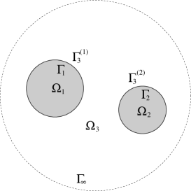
Figure 1: Geometry and notation for the BIEs. The cavity with domain $\Omega_{1}$ is bounded by the curve $\Gamma_{1}$, the one with domain $\Omega_{2}$ is bounded by $\Gamma_{2}$. The domain $\Omega_{3}$ is “bounded” by $\Gamma^{(1)}_{3}=\Gamma_{1}$, $\Gamma^{(2)}_{3}=\Gamma_{2}$ and by a circle $\Gamma_{\infty}$ at a large distance.

To reduce the two-dimensional differential equation (1) to one-dimensional integral equations, we first introduce the Green’s function, which is defined as solution of

$$[\nabla^{2}+n_{j}^{2}k^{2}]G({\bf r},{\bf r}^{\prime};k)=\delta({\bf r}-{\bf r}^{\prime})\ ,$$ (4)

where $\delta({\bf r}-{\bf r}^{\prime})$ is the two-dimensional Dirac $\delta$-function, ${\bf r}$ and ${\bf r}^{\prime}$ are arbitrary points within $\Omega_{j}$. The outgoing solution for the Green’s function is

$$G({\bf r},{\bf r}^{\prime};k)=-\frac{i}{4}H_{0}^{(1)}(n_{j}k|{\bf r}-{\bf r}^{\prime}|)\ .$$ (5)

$H_{0}^{(1)}$ is the zeroth order Hankel function of first kind GradRyzh65.

Multiplying the $\psi$-equation (1) by $G({\bf r},{\bf r}^{\prime};k)$ and subtracting the resulting equation from the $G$-equation (4) multiplied by $\psi({\bf r})$ gives

$$\psi({\bf r})\delta({\bf r}-{\bf r}^{\prime}) = \psi({\bf r})\nabla^{2}G({\bf r},{\bf r}^{\prime};k)-G({\bf r},{\bf r}^{\prime};k)\nabla^{2}\psi({\bf r})$$

$$= \nabla[\psi({\bf r})\nabla G({\bf r},{\bf r}^{\prime};k)-G({\bf r},{\bf r}^{\prime};k)\nabla\psi({\bf r})]\ .$$

Integrating this equation over the region $\Omega_{j}$ yields on the l.h.s. $\psi({\bf r}^{\prime})$ since ${\bf r}^{\prime}\in\Omega_{j}$. Applying Green’s theorem, the integral on the r.h.s. can be expressed by a line integral along the boundary curve $\Gamma_{j}=\partial\Omega_{j}$, such that

$$\psi({\bf r}^{\prime})=\oint_{\Gamma_{j}}ds[\psi(s)\partial_{\nu}G(s,{\bf r}^{\prime};k)-G(s,{\bf r}^{\prime};k)\partial_{\nu}\psi(s)]\ .$$ (6)

Note that the boundary curve may consist of a number of disconnected components $\Gamma_{j}=\Gamma^{(1)}_{j}\cup\Gamma^{(2)}_{j}\cup\ldots$ as depicted in Fig. 1. Each component is assumed to be oriented counterclockwise, smooth, and not to be a part of $\Omega_{j}$ itself, i.e. $\Omega_{j}$ is an open set. $\partial_{\nu}$ is the normal derivative defined as $\partial_{\nu}={\bf\nu}({\bf r})\nabla|_{\bf r}$; ${\bf\nu}({\bf r})$ is the outward normal unit vector to $\Gamma_{j}$ at point ${\bf r}$; $s=s({\bf r})$ is the arc length along $\Gamma_{j}$ at ${\bf r}$. The derivative of the Green’s function is given by

$$\partial_{\nu}G({\bf s},{\bf r}^{\prime};k)=\frac{in_{j}k}{4}\cos{\alpha}\,H_{1}^{(1)}(n_{j}k|{\bf r}-{\bf r}^{\prime}|)\ ,$$ (7)

where $H_{1}^{(1)}$ is the first order Hankel function of first kind GradRyzh65 and

$$\cos{\alpha}={\bf\nu}({\bf r})\frac{{\bf r}-{\bf r}^{\prime}}{|{\bf r}-{\bf r}^{\prime}|}\ .$$ (8)

The limit ${\bf r}^{\prime}\to\Gamma_{j}$ in Eq. (6) is not trivial since both the Green’s function and its normal derivative are singular at ${\bf r}^{\prime}={\bf r}$. However, it can be shown that these singularities are integrable for smooth boundaries. This is obvious for the second part of the integral kernel in Eq. (6) since for small arguments $z=n_{j}k|{\bf r}-{\bf r}^{\prime}|$

$$H^{(1)}_{0}(z)\sim\frac{2i}{\pi}\ln{z}\ .$$ (9)

The first part is also integrable. At first glance, this seems to be surprising because for small arguments

$$H^{(1)}_{1}(z)\sim-\frac{2i}{\pi z}\ .$$ (10)

However, this singularity is compensated by

$$\cos{\alpha}\sim\frac{1}{2}\kappa|{\bf r}-{\bf r}^{\prime}|\ ,$$ (11)

where $\kappa$ is the curvature of the curve $\Gamma_{j}$ at ${\bf r}(s)$, which is finite for a smooth boundary. The limit ${\bf r}^{\prime}\to\Gamma_{j}$ in Eq. (6) can be performed in the sense of Cauchy’s principal value, see e.g. Ref. KS97, giving

$$\frac{1}{2}\psi({\bf r}^{\prime})={\cal P}\oint_{\Gamma_{j}}ds[\psi(s)\partial_{\nu}G(s,{\bf r}^{\prime};k)-G(s,{\bf r}^{\prime};k)\partial_{\nu}\psi(s)]\ .$$ (12)

Comparing the l.h.s of Eqs. (6) and (12) shows that ${\bf r}^{\prime}\in\Gamma_{j}$ gives the “average” of the results for ${\bf r}^{\prime}\in\Omega_{j}$ and ${\bf r}^{\prime}\in\Omega_{i}$ with $i\neq j$.

For each region $\Omega_{j}$ there is an equation as Eq. (12). Special attention has to be paid to the unbounded region $\Omega_{J}$. It is convenient to consider instead a finite region bounded by a circle $\Gamma_{\infty}$ with a very large radius $r$ as sketched in Fig. 1. We distinguish three cases in the following subsections.

II.1 Bounded quantum states

The case of bounded states in the quantum analogue has been studied by Knipp and Reinecke KR96. Then, $n_{j}k$ has to be replaced by $[2m(E-V_{j})]^{1/2}/\hbar$, where $E$ is the energy, $V_{j}$ with $j=1,\ldots,J$ is a piece-wise constant potential, and $\hbar$ is Planck’s constant divided by $2\pi$. The wave function and its normal derivative (weighted with the inverse of the effective mass $m$) are continuous at domain boundaries. If $E<V_{J}$ then the state is bounded, the wave function and its gradient vanish exponentially as $r\to\infty$. Moreover, with $\text{Im}(k)=0$ the Green’s function (5) vanishes as either ${\bf r}$ or ${\bf r}^{\prime}$ goes to infinity. As a result $\Gamma_{\infty}$ does not contribute to any of the BIEs. Note that Eq. (1) does not permit bounded states since $n_{j}^{2}k^{2}>0$.

Using the same notation as Knipp and Reinecke KR96 we reformulate Eq. (12) as a linear homogeneous BIE

$$\oint_{\Gamma_{j}}ds[B(s^{\prime},s)\phi(s)+C(s^{\prime},s)\psi(s)]=0\ ,$$ (13)

with $B(s^{\prime},s)=-2G(s,s^{\prime};k)$, $C(s^{\prime},s)=2\partial_{\nu}G(s,s^{\prime};k)-\delta(s-s^{\prime})$, and $\phi(s)=\partial_{\nu}\psi({\bf r})$. The entire set of BIEs can be written in a symbolic way as

$$\left(\begin{array}[]{cc}B_{1}&C_{1}\\ B_{2}&C_{2}\\ \vdots&\vdots\\ B_{J}&C_{J}\end{array}\right)\left(\begin{array}[]{c}\phi\\ \psi\end{array}\right)=M\left(\begin{array}[]{c}\phi\\ \psi\end{array}\right)=0\ ,$$ (14)

where $B_{j}$ and $C_{j}$ represent the integral operators in region $\Omega_{j}$. The lower half of the vector $(\phi,\psi)^{t}$ contains the values of the wave function on the boundaries, and the upper half contains the values of the normal derivative. Note that each boundary curve has two contributions to Eq. (14) with identical $\psi$, $\phi$ (which are continuous across the boundary) but different $B_{j}$, $C_{j}$.

II.2 Plane-wave scattering

The scattering states in the related quantum problem have been discussed again by Knipp and Reinecke KR96. In contrast to the case of bounded states, their results also apply to dielectric cavities.

In region $\Omega_{J}$ the wave function has the asymptotic form as in Eq. (2). The incoming wave $\psi_{\text{in}}$ satisfies Eq. (1). Thus, $\psi$ can be replaced by $\psi-\psi_{\text{in}}$ in Eq. (6) giving

$$\psi({\bf r}^{\prime}) = \exp{(i{\bf k}{\bf r}^{\prime})}+\oint_{\Gamma_{J}}ds\{[\psi(s)-\psi_{\text{in}}(s)]\partial_{\nu}G(s,{\bf r}^{\prime};k)$$ (15)

$$-G(s,{\bf r}^{\prime};k)[\phi(s)-\phi_{\text{in}}(s)]\}\ ,$$

where $\psi_{\text{in}}(s)=\exp{(i{\bf k}{\bf r})}$ and $\phi_{\text{in}}(s)=i{\bf k}{\bf\nu}({\bf r})\exp{(i{\bf k}{\bf r})}$ at ${\bf r}={\bf r}(s)$. The circle at infinity does not contribute to the BIE (15) as in the case of bounded states. The reason, however, is different as we shall see in greater detail in the following subsection when considering resonances.

If ${\bf r}^{\prime}$ is taken from the boundary then Eq. (15) can be written as inhomogeneous integral equation

$$\oint_{\Gamma_{J}}ds[B(s^{\prime},s)\phi(s)+C(s^{\prime},s)\psi(s)] =$$

$$\oint_{\Gamma_{J}}ds[B(s^{\prime},s)\phi_{\text{in}}(s)+C(s^{\prime},s)\psi_{\text{in}}(s)] \ .$$ (16)

Together with the other $J-1$ BIEs, which are of the same form as in Eq. (13), the resulting inhomogeneous system of equations is

$$M\left(\begin{array}[]{c}\phi\\ \psi\end{array}\right)=M_{0}\left(\begin{array}[]{c}\phi_{\text{in}}\\ \psi_{\text{in}}\end{array}\right)$$ (17)

with

$$M_{0}=\left(\begin{array}[]{cc}0&0\\ \vdots&\vdots\\ 0&0\\ B_{J}&C_{J}\end{array}\right)\ .$$ (18)

Having determined the solutions $\psi$ and $\phi$ we can compute the differential scattering amplitude by evaluating Eq. (15) for large $r^{\prime}$ and comparing the result with Eq. (2) giving

$$f(\theta,{\bf k}) = \frac{1+i}{4\sqrt{\pi k}}\oint_{\Gamma_{J}}ds\exp{[-i{\bf k}_{f}{\bf r}(s)]}$$

$$\{i{\bf k}_{f}{\bf\nu}(s)[\psi(s)-\psi_{\text{in}}(s)]+\phi(s)-\phi_{\text{in}}(s)\}\ ,$$

where ${\bf k}_{f}=(k\cos\theta,k\sin\theta)$ and $\theta$ is the detection angle. Here, $|f(\theta,{\bf k})|^{2}$ is the differential scattering cross section. The total cross section $\sigma({\bf k})=\int d\theta|f(\theta,{\bf k})|^{2}$ can be easily calculated from the forward-scattering amplitude, ${\bf k}_{f}={\bf k}=(k\cos\phi,k\sin\phi)$, with the help of the optical theorem (see, e.g., Ref. Landau96)

$$\sigma({\bf k})=2\sqrt{\frac{\pi}{k}}\text{Im}[(1-i)f(\theta=\phi,{\bf k})]\ .$$ (20)

II.3 Resonances

We now turn to the BIEs for resonances. Comparing the scattering boundary condition (2) and the outgoing-wave condition (3) indicates that we possibly can use the scattering approach neglecting the incoming wave, that is Eq. (17) with $M_{0}=0$. Apart from the fact that $k$ is now a complex number, this is then identical to Eq. (14) for bounded states. There is, however, one problem. The circle at infinity, $\Gamma_{\infty}$, may give a nonvanishing contribution

$$I_{\infty}({\bf r}^{\prime})=\oint_{\Gamma_{\infty}}ds[\psi(s)\partial_{\nu}G(s,{\bf r}^{\prime};k)-G(s,{\bf r}^{\prime};k)\partial_{\nu}\psi(s)]$$ (21)

to the r.h.s. of Eq. (6) because with $\text{Im}(k)<0$ neither the wave function (3) nor the Green’s function (5) vanish at infinity. Gaspard and Rice GR89 have shown for a Dirichlet scattering problem that nonetheless $I_{\infty}({\bf r}^{\prime})=0$ if ${\bf r}^{\prime}$ is at one of the scatterers’ boundaries or if ${\bf r}^{\prime}$ is at a large distance from these boundaries. We have to extend their result because (i) the problem of dielectric cavities involves a different kind of boundary conditions; (ii) we are interested in the wave function $\psi({\bf r}^{\prime})$ also in the near-field. We start with recalling that the circle at infinity, $\Gamma_{\infty}$, is defined by $r=\text{const}$ with $r\to\infty$. Using the asymptotical behaviour of Hankel functions of first kind GradRyzh65

$$H^{(1)}_{m}(z)\sim\sqrt{\frac{2}{\pi z}}\exp{[i(z-m\pi/2-\pi/4)]}$$ (22)

as $z=k|{\bf r}-{\bf r^{\prime}}|\to\infty$, it can be shown that the Green’s function in Eq. (5) is asymptotically given by

$$G({\bf r},{\bf r}^{\prime};k)\sim g(\theta-\theta^{\prime},r^{\prime})\frac{\exp{(ikr)}}{\sqrt{r}}\ ,$$ (23)

with

$$g(\theta-\theta^{\prime},r^{\prime})=-\frac{1+i}{4\sqrt{\pi k}}\exp{[-ikr^{\prime}\cos{(\theta-\theta^{\prime})}]}\ .$$ (24)

Equation (23) has the same $r$-dependence as the outgoing-wave condition (3). With $G$ and $\psi$ appearing in Eq. (21) in an antisymmetric way it follows $I_{\infty}({\bf r}^{\prime})=0$ for all ${\bf r}^{\prime}\in\Omega_{J}\cup\Gamma_{J}$. The fact that $I_{\infty}({\bf r}^{\prime})$ vanishes for ${\bf r}^{\prime}\in\Gamma_{J}$ means that the BIEs (14) can indeed be used to determine the resonant wave numbers $k$. Moreover, since $I_{\infty}({\bf r}^{\prime})=0$ also for ${\bf r}^{\prime}\in\Omega_{J}$ Eq. (6) can be used to compute the corresponding wave functions in the entire domain.

Having established that the resonances are solutions of the BIEs (14) with complex-valued $k$, we now demonstrate that the BIEs (14) posses additional solutions which do not fulfil the outgoing-wave condition (3). We study this in an elementary way for a single cavity of arbitrary shape. Outside this cavity sufficiently far away from its boundary, a solution of wave equation (1) can be expressed as

$$\psi(r,\theta)=\sum_{m=-\infty}^{\infty}[\alpha_{m}^{(1)}H^{(1)}_{m}(kr)+\alpha_{m}^{(2)}H^{(2)}_{m}(kr)]\exp{(im\theta)}\ ,$$ (25)

with Hankel functions of first and second kind GradRyzh65 and with unknown complex-valued parameters $\alpha_{m}^{(1)}$ and $\alpha_{m}^{(2)}$. Without boundary conditions at infinity, solutions as in Eq. (25) exist for all values of $k$. Boundary conditions that fix all parameters $\alpha_{m}^{(2)}$ give rise to a discrete spectrum of $k$; for instance, the outgoing-wave condition (3) requires $\alpha_{m}^{(2)}=0$ for all $m$. Inserting the expansion (25) into Eq. (21) leads to

$$I_{\infty}({\bf r}^{\prime})=2\sum_{m=-\infty}^{\infty}\alpha_{m}^{(2)}J_{m}(kr^{\prime})\exp{(im\theta^{\prime})}\ .$$ (26)

Hence, $I_{\infty}({\bf r}^{\prime})$ vanishes identically for all ${\bf r}^{\prime}\in\Omega_{J}\cup\Gamma_{J}$ only in the case of a resonance, where $\alpha_{m}^{(2)}=0$ for all $m$.

However, the circle at infinity does not contribute to the BIEs (14) already if the weaker condition $I_{\infty}({\bf r}^{\prime})=0$ for ${\bf r}^{\prime}\in\Gamma_{J}$ is satisfied. We insert this condition into the l.h.s. of Eq. (26) and note that the r.h.s. is an expansion of a solution of wave equation (1) inside the cavity with “wrong” index of refraction $n=n_{J}=1$. The result is that the BIEs (14) possess undesired solutions, namely bounded states of an interior Dirichlet problem, in addition to the resonances. As one consequence, the solutions of the scattering BIEs (17) are not unique whenever $k$ is a solution of the interior Dirichlet problem. Note that this nonuniqueness has not been discussed by Knipp and Reinecke KR96.

A related problem is known for cases with Dirichlet or Neumann conditions; see, e.g., Refs. CB91; CZ92. There have been several attempts to modify the BIEs in order to get rid of these “spurious solutions”. Some of these modifications could be applied to the present case, but this would result in singular integrals which are hard to deal with numerically. Fortunately, the spurious solutions are not a severe problem for our purpose. We can distinguish them, in principle, from the resonances in which we are interested in. The former have $\text{Im}(k)=0$ whereas the latter have $\text{Im}(k)<0$.

II.4 TE polarization

In the case of TE polarization, Eq. (1) is valid with $\psi$ representing the magnetic field $H_{z}$. The wave function $\psi$ is continuous across the boundaries, but its normal derivative is not, in contrast to the case of TM polarization. Instead, $n({\bf r})^{-2}\partial_{\nu}\psi$ is continuous Jackson83.

This new boundary condition can be easily incorporated in the BEM by defining $\phi=n^{-2}\partial_{\nu}\psi$, $B(s^{\prime},s)=-2G(s,s^{\prime};k)n^{2}$ and $\phi_{\text{in}}$ accordingly in equations like Eqs. (13) and (16). We remark that the spurious solutions are not affected by this change of boundary conditions.

II.5 Symmetry considerations

Many dielectric cavities studied in the literature possess discrete symmetries. For example, the elliptical cavity in Fig. 2 is symmetric with respect to the $x$ and $y$ axes. In such a case, the wave functions can be divided into four symmetry classes

$$\psi_{\zeta\xi}(-x,y) = \zeta\psi_{\zeta\xi}(x,y)\ ,$$ (27)

$$\psi_{\zeta\xi}(x,-y) = \xi\psi_{\zeta\xi}(x,y)\ ,$$ (28)

with the parities $\zeta\in\{-,+\}$ and $\xi\in\{-,+\}$. The normal derivative obeys the same symmetry relations.

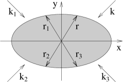
Figure 2: Symmetric cavity.

For systems with symmetries the BIEs can be reduced to a fundamental domain if a modified Green’s function is used. This decreases the numerical effort considerably. Let us restrict our discussion to the case in Eqs. (27) and (28); other symmetries can be treated in a similar way. The BIEs (12) reduce to integrals along the boundaries restricted to the quadrant $x,y\geq 0$ if the Green’s function $G({\bf r},{\bf r}^{\prime})$ is replaced by

$$G({\bf r},{\bf r}^{\prime})+\zeta G({\bf r}_{1},{\bf r}^{\prime})+\zeta\xi G({\bf r}_{2},{\bf r}^{\prime})+\xi G({\bf r}_{3},{\bf r}^{\prime})$$ (29)

with ${\bf r}=(x,y)$, ${\bf r}_{1}=(-x,y)$, ${\bf r}_{2}=(-x,-y)$, ${\bf r}_{3}=(x,-y)$; see Fig. 2. The derivative $\partial_{\nu}G(s,{\bf r}^{\prime})$ is modified in the same way with the normal unit vector ${\bf\nu}$ changing as ${\bf r}$.

The scattering problem as formulated in Sec. II.2 does not allow the symmetry reduction because the incoming plane wave in general destroys the symmetry; $\phi_{\text{in}}$ and $\psi_{\text{in}}$ in Eq. (17) do not fulfil the conditions (27) and (28). There are certain incoming directions which do not spoil the symmetry, but using only these special directions is dangerous because possibly not all resonances are excited. A better approach is to consider a different physical situation illustrated in Fig. 2. Four plane waves are superimposed to a symmetric incoming wave

$$\psi_{\text{in}}=\exp{(i{\bf k}{\bf r})}+\zeta\exp{(i{\bf k}_{1}{\bf r})}+\zeta\xi\exp{(i{\bf k}_{2}{\bf r})}+\xi\exp{(i{\bf k}_{3}{\bf r})}$$ (30)

where ${\bf k}=(k_{x},k_{y})$, ${\bf k}_{1}=(-k_{x},k_{y})$, ${\bf k}_{2}=(-k_{x},-k_{y})$, ${\bf k}_{3}=(k_{x},-k_{y})$. With this incoming wave, the scattering problem can be symmetry reduced. A more general formulation for an arbitrary symmetry can be found in Ref. ND94.

III Boundary element method

The most convenient numerical strategy for solving BIEs as in Eqs. (13) and (16) is the BEM. The boundary is discretized by dividing it into small boundary elements. Along such an element, the wave function and its normal derivative are considered as being constant (for linear, quadratic, and cubic variations see, e.g., Refs. CB91; Banerjee94). Equation (13) is therefore approximated by a sum of $N_{j}$ terms

$$\sum_{l=1}^{N_{j}}(B_{il}\phi_{l}+C_{il}\psi_{l})=0$$ (31)

where $B_{il}=\int_{l}ds\,B(s_{i},s)$, $C_{il}=\int_{l}ds\,C(s_{i},s)$, $\phi_{l}=\phi(s_{l})$, $\psi_{l}=\psi(s_{l})$, and $\int_{l}$ denotes the integration over a boundary element with midpoint $s_{l}$. The entire set of BIEs is approximated by an equation as in Eq. (14), but for which $B_{j}$ and $C_{j}$ are $N_{j}\times N$ matrices, $M$ is a $2N\times 2N$ (non-Hermitian complex) matrix, $\phi$ and $\psi$ are $N$-component vectors with $2N=\sum_{j=1}^{J}N_{j}$. Note that each boundary element belongs to two different regions. In the same way the scattering problem is approximated by an equation as in Eq. (17) with $M_{0}$ being a $2N\times 2N$ matrix, $\phi_{\text{in}}$ and $\psi_{\text{in}}$ being $N$-component vectors.

In the literature several levels of approximation are used for the matrix elements $B_{il}$ and $C_{il}$. The crudest approximation is to evaluate such an integral only at the corresponding midpoint $s_{l}$. While this is sufficient for the calculation of bounded states in quantum billiards Baecker02, in our case the small imaginary parts of $k$ require a more accurate treatment. We therefore do perform the numerical integration of the matrix elements $B_{il}$ and $C_{il}$, using standard integration routines like, for example, Gaussian quadratures Press88. The number of interior points in the range of integration should be chosen large if the boundary elements $s_{i}$ and $s_{l}$ are close to each other and small if they are far away. Moreover, our experience is that the results are considerably more accurate if the boundary elements are not approximated by straight lines but, instead, the exact shape of the boundary elements is used for all interior points in the range of integration.

Due to the almost singular behaviour of the integral kernels at ${\bf r}^{\prime}={\bf r}$, the diagonal elements $C_{ll}$ and $B_{ll}$ require special care. Inserting the limiting cases for small boundary-element length $\Delta s_{l}$ in Eqs. (10) and (11) into Eq. (7) gives

$$C_{ll}=-1+\frac{\kappa_{l}}{2\pi}\Delta s_{l}\ ,$$ (32)

where $\kappa_{l}$ is the curvature at point $s_{l}$. To approximate $B_{ll}$ accurately, more higher order terms than in Eq. (9) are needed:

$$H^{(1)}_{0}(z)\sim\frac{2i}{\pi}\ln{\frac{z}{2}}+1+\frac{2i}{\pi}\gamma\ ,$$ (33)

where $\gamma=0.577215\ldots$ is Euler’s constant. Integration yields

$$B_{ll}=\frac{\Delta s_{l}}{\pi}[1-\ln{\frac{n_{j}k\Delta s_{l}}{4}}+i\frac{\pi}{2}-\gamma]\ .$$ (34)

III.1 Treatment of corners

Dielectric corners are numerically difficult to treat because certain components of the electric field can be infinite at the corner (see the discussion in Ref. Hadley02 in the context of dielectric waveguides). In the BEM, a corner leads to a second problem. The integral kernel of $C_{ll}$ has a singularity caused by a diverging curvature $\kappa$; see Eq. (11). To circumvent these difficulties, we smooth the boundary as sketched in Fig. 3. The curvature $\kappa$ and the electric field are then everywhere bounded.

The minimum value of the radius of curvature, $\rho=1/\kappa$, along such a rounded corner should be much larger than the typical distance between discretization points, so that the boundary is locally smooth. However, in order to ensure that the rounding does not influence the result, $\rho$ should be much smaller than the wavelength $\lambda$. Clearly, these requirements can be met most efficiently by using a nonuniform discretization with a relatively large density of discretization points at corners as illustrated in Fig. 3. Since the results do not depend on the particular selected rounding and discretization we do not give explicit formulae.

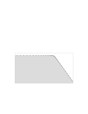
Figure 3: Rounded corner. The number of discretization points (circles) is enhanced at the corner.

III.2 Finding and computing resonances

The scattering problem as discussed in Sec. II.2 provides us with first approximations to the wave numbers of the resonances. Let us fix $\phi$ to an appropriate value and plot the total cross section in Eq. (20) as function of $k$ in the range of interest. Resonances can be identified as peaks. The peak position $\alpha$ and the width $\gamma$ determine the resonant wave number as $k_{\text{res}}\approx k_{1}=\alpha-i\gamma/2$. It might be difficult to resolve numerically very broad and very narrow peaks, because they are hidden either in the background or between two consecutive grid points. For microlaser operation, however, these two extreme cases are not relevant. Too short-lived resonances (broad peaks) fail to provide a sufficient long lifetime for the light to accumulate the gain required to overcome the lasing threshold, whereas too long-lived resonances (narrow peaks) do not supply enough output power.

The spurious solutions of the interior Dirichlet problem occasionally appear in the scattering spectrum as extremely narrow peaks. The reason is that numerical inaccuracies broaden the $\delta$-peaks to peaks of finite width. However, choosing a sufficiently fine boundary discretization and/or an appropriate, not too fine discretization in $k$ reduces the probability of observing them. Moreover, they can be removed with a simple trick: use $k$ with a small negative imaginary part in Eq. (20).

The discretized version of Eq. (14) has a nontrivial solution only if $\det{M(k_{\text{res}})}=0$. Using a first approximation $k_{1}$ from the scattering problem as starting value, we find a much better approximation to $k_{\text{res}}$ in the complex plane with the help of Newton’s method

$$k_{l+1}=k_{l}-\frac{g(k_{l})}{g^{\prime}(k_{l})}$$ (35)

with $l=1,2,\ldots$ and $g(k)=\det{M(k)}$. The derivative $g^{\prime}(k)=\partial g(k)/\partial k$ can be approximated by

$$g^{\prime}(k)\approx\frac{g(k+\Delta)-g(k)}{2\Delta}-i\frac{g(k+i\Delta)-g(k)}{2\Delta}\ ,$$ (36)

where $\Delta$ is a small real number. Equation (35) is repeated iteratively until a chosen accuracy is achieved.

Newton’s method in Eq. (35) is very efficient close to an isolated resonance where $\det{M}\propto k-k_{\text{res}}$. For $q$-fold degenerate resonances the determinant behaves like $(k-k_{\text{res}})^{q}$. The resulting problem of slow convergence can be eliminated by choosing $g=(\det{M})^{1/q}$.

A slightly different approach for finding resonances can be gained by rewriting Newton’s method in Eq. (35) with the help of the matrix identity $\ln\det{M}=\text{tr}\ln{M}$ as

$$k_{l+1}=k_{l}-\frac{q}{\text{tr}[M^{-1}(k_{l})M^{\prime}(k_{l})]}\ ,$$ (37)

where tr denotes the trace of a matrix. The derivative $M^{\prime}(k)$ can be calculated as in Eq. (36). It turns out that the numerical algorithm corresponding to Eq. (37) is a bit faster than the original Newton’s method in Eq. (35).

Having found a particular wave number $k_{\text{res}}$, the vector components $\phi_{l}$ and $\psi_{l}$ are given by the null eigenvector of the square matrix $M(k_{\text{res}})$. This eigenvector can be found with, for instance, singular value decomposition Press88. The wave function in each domain $\Omega_{j}$ is then constructed by discretizing Eq. (6)

$$\psi({\bf r}^{\prime}) = \sum_{l}\psi_{l}\int_{l}ds\,\partial_{\nu}G(s,{\bf r}^{\prime};k_{\text{res}})$$

$$-\sum_{l}\phi_{l}\int_{l}ds\,G(s,{\bf r}^{\prime};k_{\text{res}})\ ,$$

where $l$ runs over all boundary elements of $\Gamma_{j}$.

How fine must be the discretization of the boundary in order to obtain a good approximation of a resonance at $k_{\text{res}}$? The local wavelength $\lambda=2\pi/n\text{Re}(k_{\text{res}})$ is the smallest scale on which the wave function and its derivative may vary. Hence, the minimum number of boundary elements along each wavelength, $b=\lambda/\Delta s$, should be larger or equal than at least $4$; $\Delta s$ is the maximum value of all lengths $\Delta s_{i}$. We have verified the BEM using different values of $b$. Taking $b=16$, we find good agreement with the separation-of-variables solution of the circular cavity (see e.g. Ref. BarberHill90) and to results of the wave-matching method obtained for the quadrupolar cavity ND97. Only for extremely long-lived resonances larger $b$ are necessary to determine the very small imaginary parts of $k$ accurately (recall that this is important for distinguishing spurious solutions from real resonances). However, as already explained, extremely long-lived resonances are not relevant for microlaser applications and, moreover, they occur only in circular or slightly deformed circular cavities for which the wave-matching method is more suitable anyway.

IV Example: two coupled hexagonal-shaped cavities

Vietze et al. have experimentally realized hexagonal-shaped microlasers by putting laser active dyes into molecular sieves made of ${\text{AlPO}_{4}-5}$ VKLISLA98. Numerical simulations on rounded hexagons based on the wave-matching method have shown convergence problems at corners BILNSSVWW00; Noeckelpc02. The following example is relevant for future experiments and demonstrates that the BEM can handle arbitrarily sharp corners and, moreover, coupled resonators. Near-field-coupling of resonators is interesting, because it may improve the optical properties of the resonators, as e.g. the far-field directionality.

Figure 4 illustrates the configuration: two hexagonal cavities with sidelength $R$ are displaced by the vector $(1.8R,0.5R)$. According to the experiments in Ref. VKLISLA98; BILNSSVWW00, the polarization is of TM type, the index of refraction is $n=1.466$ inside the cavities and $n=1$ outside; $R$ ranges from $4\mu\text{m}$ to $10\mu\text{m}$, the wavelength $\lambda$ from $600\text{nm}$ to $800\text{nm}$ depending on the dye. Since only the ratio between $R$ and $\lambda$ is relevant, we use in the following the dimensionless wave number $kR$. We focus on a $kR$-interval from $20$ to $25$ within the experimental spectral interval. A total of $2N=3200$ discretization points is then sufficient. We slightly smooth the corners as discussed in Sec. III.1 such that $\rho/\lambda\approx 0.11$ and $\rho/\Delta s\approx 11.2$.

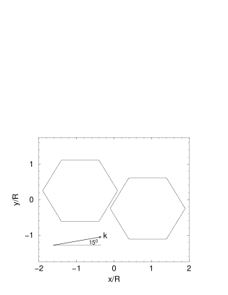
Figure 4: Two hexagonal cavities. The incoming plane wave with wave vector ${\bf k}$ is incidence at $15^{\circ}$ to the horizontal side faces.

Figure 5 shows the total cross section $\sigma$ for plane-wave scattering with incidence angle $\phi=15^{\circ}$ computed from Eq. (20). The dominant structure is a series of equidistant peaks of roughly Lorentzian shape. At $kR\approx 23.25$ we identify a spurious solution of the interior Dirichlet problem. The fact that it is the only one visible in the chosen range of wave numbers confirms that the spurious solutions are not a problem.

Figure 5: Calculated total cross section $\sigma/R$ vs. $kR$ for two coupled hexagonal resonators. The plane wave is incidence at $15^{\circ}$ to the horizontal side faces; cf. Fig. 4.

The peak at $kR\approx 22.95$ in Fig. 5 has roughly the width $0.196$, so we use $k_{1}R=22.95-i0.098$ as initial guess for Newton’s method in Eq. (37). The more precise location of the resonance is found to be $k_{\text{res}}R\approx 22.94444-i0.09696$. The near-field intensity pattern in Fig. 6 and the far-field emission pattern in Fig. 7 are computed with the help of Eq. (III.2). A detailed account of the structure of this kind of resonances and its implication on the properties of the microlasers will be given in a future publication.

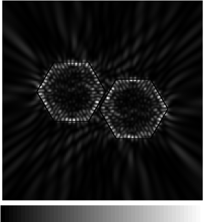
Figure 6: Calculated near-field intensity pattern $|\psi({\bf r})|^{2}$ of the resonance with $k_{\text{res}}R\approx 22.94444-i0.09696$. Intensity is higher for light regions and vanishes in the black regions.

Figure 7: Far-field emission pattern, $|\psi(r,\theta)|^{2}$ with large $r$, of the resonance in Fig. 6.

V Summary

We have introduced a boundary element method (BEM) to compute TM and TE polarized resonances with intermediate lifetimes in dielectric cavities. We have discussed spurious solutions, the treatment of cavities with symmetries and cavities with corners. Numerical results are shown for an example of two coupled hexagonal cavities.

If compared to finite-difference methods and related methods the BEM is very efficient since the wave function and its derivative are only evaluated at the boundaries of the cavities. It is in general less efficient than the wave-matching method but in contrast to the latter it can be applied to complex geometries, such as cavities with corners and coupled cavities.

The BEM is especially suitable for computing phase space representations of wave functions such as the Husimi function which also only requires the wave function and its normal derivative on the domain boundaries HSS02.