Numerical computation of critical properties and atomic basins from 3D grid electron densities

Abstract

InteGriTy is a software package that performs topological analysis following AIM approach on electron densities given on 3D grids. Use of tricubic interpolation is made to get the density, its gradient and hessian matrix at any required position. Critical points and integrated atomic properties have been derived from theoretical densities calculated for the compounds NaCl and TTF-2,5Cl₂BQ, thus covering the different kinds of chemical bonds: ionic, covalent, hydrogen bonds and other intermolecular contacts.

InteGriTy, a software package to compute topological properties of electron densities given on 3D grids.

1 Introduction

Nowadays, very accurate electron densities can be obtained both experimentally and theoretically. Experimental methods of recovering charge densities require high resolution X-ray diffraction measurements on single crystals which are analysed within the context of aspherical models. From the theoretical point of view, not only crystals but also molecules, clusters and surfaces can be tackled using either quantum chemistry techniques ranging from standard Hartree-Fock calculations up to extremely accurate configuration interaction methods or techniques based on the Density Functional Theory (DFT) which are increasingly used to perform ab-initio calculations. Once the total electron density is known, it can be analyzed in details by means of its topological properties within the Quantum Theory of Atoms in Molecules (Bader, 1990; Bader, 1994). With such an analysis one can go beyond a purely qualitative description of the nature and strength of interatomic interactions. It can also be used to define interatomic surfaces inside which atomic charges and moments are integrated.

The topological features of the total electron density $\rho(\mathbf{r})$ can be characterized by analyzing its gradient vector field $\mathbf{\nabla}\rho(\mathbf{r})$. Critical points (CPs) are located at points $\mathbf{r}_{\mbox{\scriptsize CP}}$ where $\mathbf{\nabla}\rho(\mathbf{r}_{\mbox{\scriptsize CP}})=\mathbf{0}$ and the nature of each CP is determined from the curvatures ($\lambda_{1}$, $\lambda_{2}$, $\lambda_{3}$) of the density at this point. The latter are obtained by diagonalyzing the Hessian matrix $H_{ij}={\partial^{2}\rho(\mathbf{r})\over\partial x_{i}\partial x_{j}}(i,j=1,2,3)$. The CPs are denoted by a pair of integers $(\omega,\sigma)$ where $\omega$ is the number of non-zero eigenvalues of the Hessian matrix $H(\mathbf{r})$ and $\sigma$ the sum of the signs of the three eigenvalues. In a three dimensional stable structure, four types of CPs can be found: $(3,-3)$ Peaks corresponding to local maxima of $\rho(\mathbf{r})$ which occur at atomic nuclear positions and in rare cases at so called non-nuclear attractors; $(3,-1)$ Passes, corresponding to saddle points where $\rho(\mathbf{r})$ is maximum in the plane defined by the axes corresponding to the two negative curvatures and minimum in the third direction, such bond critical points are found between pairs of bonded atoms; $(3,+1)$ Pales where $\rho(\mathbf{r})$ is minimum in the plane defined by the axes associated with the two positive curvatures and maximum in the third direction, such ring critical points are found within rings of bonded atoms; $(3,+3)$ Pits corresponding to local minima of $\rho(\mathbf{r})$. The numbers of each type of CPs obbey the following relationship depending on the nature of the system: $N(\mbox{peaks})-N(\mbox{passes})+N(\mbox{pales})-N(\mbox{pits})=0$ or $1$ for a crystal or an isolated system respectively. The Laplacian of the electron density $\nabla^{2}\rho(\mathbf{r})$ which is given by the trace of $H(\mathbf{r})$ is related to the kinetic and potential electronic energy densities, respectively G($\mathbf{r}$) and V($\mathbf{r}$), by the local virial theorem,

$${1\over 4}\nabla^{2}\rho(\mathbf{r})=2G(\mathbf{r})+V(\mathbf{r})$$

(atomic units are used throughout the paper). The sign of the laplacian at a given point determines whether the positive kinetic energy or the negative potential energy density is in excess. A negative (positive) Laplacian implies that density is locally concentrated (depleted). Within the Quantum Theory of Atoms in Molecules, a basin is associated to each attractor $(3,-3)$ CP, defined as the region containing all gradient paths terminating at the attractor. The boundaries of this basin are never crossed by any gradient vector trajectory and satisfy $\mathbf{\nabla}\rho(\mathbf{r})\cdot\mathbf{N}(\mathbf{r})=0$, where $\mathbf{N}(\mathbf{r})$ is the normal to the surface at point $\mathbf{r}$. The corresponding surface is called the zero flux surface and defines the atomic basin when the attractor corresponds to a nucleus. Only in very rare cases non-nuclear attractors have been evidenced (Madsen et al., 1999). Within this space partionning, the atomic charges deduced by integration over the whole basin are uniquely defined.

During the last twenty years, several programs have been developped to perform topology of electron densities but they are either connected to computer program packages (Gatti et al., 1994; Koritsanszky et al., 1995; Souhassou et al., 1999; Stash et al., 2001; Stewart et al. 1983; Volkov et al., 2000) or have limitations concerning the type of wavefunctions which have been used to determine $\rho(\mathbf{r})$ in ab-initio calculations (Barzaghi, 2001; Biegler König et al., 1982; Biegler König et al., 2001; Popelier, 1996 ) or to refine experimental data (Barzaghi, 2001). To our knowledge,only two cases were described to analyse the topology of $\rho(\mathbf{r})$ numerically on grids; Iversen et al. (Iversen et al., 1995) used a maximum entropy density and Aray et al. (Aray et al., 1997) sampled a theoretical density on a homogeneous grid. However, these approaches are limited to the determination of CPs. The present analysis of the topological features of total electron densities is independent of the way these densities are obtained and works for periodic or non-periodic systems. We show in this paper that this can be simply achieved by working with densities given on regular grids in real space. The developed software InteGriTy uses a tricubic Lagrange interpolation which makes the CP search and integration method both accurate and fast. The densities used to illustrate the performance of our approach are theoretical ab-initio densities obtained with the Projector Augmented Wave (PAW) method (Blöchl, 1994). The next section of this paper gives a short description of the method. Test compounds and computational details are given in Section 3. Section 4 is devoted to the determination of CPs and their characteristics whereas section 5 concerns the determination of atomic basins and charges. We will discuss the effect of grid spacing of the input density and the plane wave cutoff used for the PAW calculations on the properties of different type of interactions (ionic, covalent and intermolecular).

2 Description of the method

2.1 Input data and interpolation

In order to achieve the topological analysis of any experimental or theoretical electron density, the density is given on a regular, not necessarily homogeneous grid in real space. A grid of stored values of $\rho(\mathbf{r})$ must be prepared, preferably in binary format in order to save disk space and with double precision to ensure high precision. The grid which is defined by its origin, three meshgrid vectors and the number of points in each grid direction as well as atomic positions must be specified with respect to a cartesian coordinate system. Determinations of the topological properties of $\rho(\mathbf{r})$ requires the knowledge of $\rho(\mathbf{r})$, $\mathbf{\nabla}\rho(\mathbf{r})$ and $H(\mathbf{r})$ at many arbitrary points. This can be achieved in an accurate and efficient way by using a tricubic Lagrange interpolation (Press et al., 1992). In one dimension, it uses values of $\rho$ on two grid points on each side of the current point as illustrated in figure 1. For a three-dimensional system, it uses 64 grid points surrounding the box containing the current point:

$$\rho(x,y,z)=\sum_{i=1}^{4}\sum_{j=1}^{4}\sum_{k=1}^{4}\rho(i,j,k)\,L_{i}(x)\,L_{j}(y)\,L_{k}(z).$$

As the first and second derivatives of this expression are straighforward, the evaluation of $\mathbf{\nabla}\rho(\mathbf{r})$ and $H(\mathbf{r})$ is numerically very cheap. It is clear that with respect to analytical expressions, the interpolation may introduce errors. However, as shown in section 4 and 5 these errors are small for reasonable values of the grid interval size, and insignificant when compared to those issued from the multipolar refinement of experimental structure factors. One should also notice that this interpolation is not suited to perform the topology of $\nabla^{2}\rho(\mathbf{r})$ from the density. Higher order interpolation would be required or the Laplacian has to be supplied on a grid.

Figure 1: One dimensional example for tricubic Lagrange interpolation. $x_{i}$ and $\rho_{i}$ are respectively the abscissa and density value at grid point $i$. The density at the current abscissa $x$ is given by $\rho(x)$ where $L_{i}(x)$ are third order polynomial, passing through all the grid points as shows the example of $L_{1}(x)$.

2.2 Critical points

To locate the CPs, starting from every grid point, a standard Newton-Raphson technique (Press et al., 1992) is used to find the zero’s of its gradient modulus:

$$\mathbf{r}_{i+1}=\mathbf{r}_{i}-\alpha\;H^{-1}(\mathbf{r}_{i})\cdot\mathbf{\nabla}\rho(\mathbf{r}_{i}).$$

Far from the CPs, the full Newton step will not necessarily decrease the gradient modulus and the parameter $\alpha$ allows the stepsize adjustment. In all our calculations an $\alpha$ value of $0.3$ led to stable results. This iterative procedure is used until the gradient modulus becomes less than a choosen threshold value. The corresponding CP is then stored if no other CP has been found in its vinicity. Otherwise, the program keeps the point which has the smallest gradient modulus. The CPs can then be classified with respect to their type and/or to the magnitude of $\rho(\mathbf{r}_{\mbox{\scriptsize CP}})$. It is worth emphasizing that, since each grid point acts in its turn as a starting point, CP search does not require a priori knowledge of atom location, nor the definition of plane or local coordinates system. Periodic boundary conditions are used to treat periodic systems whereas four grid points at each border of the input box are ignored in the case of non periodic systems.

2.3 Atomic Basins

Interpolation of electronic density on grid can also be used to derive atomic basins and integrate the density to obtain the atomic charges with good accuracy and reasonable computer time. The surface $S_{\Omega}$ of each basin $\Omega$ is determined by its intersection with rays originating from the attractor. Only one intersection per ray is looked for. Then the determined surfaces may not be fully correct (Biegler König et al., 1982; Popelier, 1998) but the missing volume that can be checked a posteriori is very low, thus having no appreciable effect on the integrated charges. Basin search is performed on total density whereas highly accurate integration is obtained from valence part only to avoid using unreasonably small grid steps. The program works with both periodic and non periodic conditions for the input grids and a threshold electron density value can be applied to limit the surface of open systems (e.g. van der Waals envelope, Bader, 1990). The present integration results concern only periodic systems thus allowing a posteriori validation of the process according to the sum over the whole unit cell of all basin volumes, including all atoms and possible non nuclear attractors.

Figure 2: Schematic diagram to illustrate how a running point in radial coordinates is checked following the gradient path inside $\left(\bullet\right)$ or outside $\left(\circ\right)$ a basin centered on the attractor A and delimited by the surface $S_{\Omega}$. $\mathbf{r}_{A}$ and $\mathbf{r}$ respectively give the positions of the attractor and the running point in the absolute cartesian coordinates system. The incremental step length $g\,dr_{o}$ is defined in the text.

2.3.1 Basin search

To search for the surface of a basin, a radial coordinates system centered on each attractor is used and one point of the basin surface $R_{\Omega}\left(\theta,\phi\right)$ is looked for along the ray defined by $\theta$ and $\phi$ angles. A point $r\left(\theta,\phi\right)$ is declared inside the basin $\Omega$ if the following gradient path brings it towards a sphere centered on the attractor and with radius $R_{min}$ small enough to be in the basin, as illustrated in figure 2. The running point is declared outside of $\Omega$ if a few iteration steps successively move it away from the attractor. The step amplitude used to follow the gradient is the product of a minimum step $dr_{0}$ weighted by a coefficient $g$ depending on the angle $\omega$ between the considered ray and the gradient. It takes the form $ln\left(g\right)=A\mid cos\left(\omega\right)\mid^{B}$ so that the maximum step size corresponds to the parallel situation. The search algorithm used for each ray is given in figure 3. A coarse bracketing, $R_{low}<R_{\Omega}\left(\theta,\phi\right)<R_{high}$, is first performed starting from the value $R_{start}$ and using geometric progression with common ratio $1+\nu$. The sign and amplitude of $\nu$ depends on wether bracketing is done downward to or away from the attractor. A dichotomy procedure is then used to refine the $R_{\Omega}\left(\theta,\phi\right)$ value with predefined tolerance $d_{tol}$. At the first $\left(\theta,\phi\right)$ step, $R_{start}$ is set to an arbitrary value given for each atom as an input parameter. A crude estimation of basins limits is done first on a regular $\left(\theta,\phi\right)$ grid with small number of points $n_{\theta}$ and $n_{\phi}=2n_{\theta}$ with each $R_{\Omega}\left(\theta,\phi\right)$ acting as starting value for the next $\left(\theta,\phi\right)$ step. This search is sufficient for graphical purpose and enables $R_{start}$ initialisation by linear interpolation at all $\left(\theta,\phi\right)$ points added during the integration process. The $R_{min}$ value is updated at the end of the crude estimation in order to save time during integration process. It is automatically reset to a lower value where it needs to be so.

Figure 3: Basin surface location flowchart for a given ray originating from an attractor with spherical coordinates $\theta$ and $\phi$. $L$ and $H$ are dummy logical constants to check if both the low and high limits of the coarse bracketting have been found. In the second part of the flowchart, the dichotomy process is stopped when the distance between the two limits is below the predefined tolerance $d_{tol}$.

2.3.2 Integration

Two methods can be used for integration, both using three nested integration do loops with spherical coordinates. The first one is straightforward and uses the same fixed number of $\left(\theta,\phi,r\right)$ points for all attractors. The number $n_{r}$ and $n_{\theta}$ of radial and $\theta$ steps are kept fixed, whereas the number $n_{\phi}\left(\theta\right)$ of $\phi$ steps is $\theta$ dependent such that elementary solid angle $sin\left(\theta\right)\delta\theta\delta\phi$ be constant. The integral $Q_{f}$ of a quantity $f\left(\theta,\phi\\ ,r\right)$ is simply given by the discrete sum:

$$Q_{f}=\delta r\,\delta\theta\,\sum_{i=1}^{n_{\theta}}sin\left(\theta_{i}\right)\delta\phi\left(\theta_{i}\right)\sum_{j=1}^{n_{\phi}\left(\theta_{i}\right)}\sum_{k=1}^{n_{r}}r_{k}^{2}\,f\left(\theta_{i},\phi_{j},r_{k}\right)$$

The second method uses Romberg procedure (Press et al., 1992) and is illustrated in figure 4 for a single variable function $f$ to be integrated in the interval $[a,b]$.

Figure 4: Romberg flowchart for the integration of a function $f$ in the interval $[a,b]$. $Q_{f}$ stands for an integrated property (charge, laplacian,volume) at the three imbricated levels of integration, namely: radial, $\phi$ and $\theta$ in the respective intervals $[0,R_{\Omega}\left(\theta,\phi\right)]$, $[0,2\pi]$ and $[0,\pi]$.

It first calculates an estimation of the integral $Q_{f}$ over $n$ stages of the extended trapezoidal rule with successive integration steps $\{h_{n}\}$ and extrapolates $Q_{f}$ with $k$ order polynomial in $h^{2}$ to the continuum limit $h=0$ over the last $n-k$ stages. The interpolation starts after n$\geq k_{min}$ stages. This iterative process is terminated when either an estimated error $\sigma$ derived from the extrapolation operation yields a desired relative accuracy $\epsilon$ such that $\sigma\leq(\epsilon\cdot Q_{f})$ or a fixed maximum number of stages $n_{max}$ is reached. Several convergence criteria can be used for the radial, $\phi$ and $\theta$ levels of integration. Total and valence atomic charges, volume and laplacian are integrated and convergence criteria can be choosen on each of these quantities. Individual quantities are summed up at the end of the loop over all attractors. Total charges and volume are then compared to the expected ones and residuals give the accuracy of the integration process.

3 Test compounds

Different types of crystals and molecules have been used to test limits, accuracy and performance of algorithm. In this paper, we have selected two crystals, NaCl a classical example for ionic crystals, and TTF-2,5Cl₂BQ for covalent and intermolecular interactions. The latter compound was also chosen for the following reasons: with 26 atoms in the unit cell the system is neither too small nor too large; the unit cell is triclinic then the grid will not be orthogonal; the presence of inversion symmetry should be recovered in all properties; finally the expected small intermolecular charge transfer (about 0.5 out of 200 electrons) is a good quantity to test for the accuracy of charge integration.

Figure 5: Representation of a mixed stack of alternating TTF and 2,5Cl₂BQ molecules including atomic numbering. Open circles indicate bond and ring CPs. The lines connecting two molecules correspond to bond paths determined by following $\mathbf{\nabla}\rho(\mathbf{r})$ with a small stepsize. Diamonds indicate some intermolecular $(3,-1)$ CPs.

All calculations used to generate the electron densities were carried out with the Projector Augmented Wave (PAW) method (Blöchl, 1994), an all-electron code developped by P. E. Blöchl. The wave functions were expanded into augmented plane wave up to a kinetic energy (E${}_{\mbox{\scriptsize cutoff}}$) ranging from 30 to 120 Ry. NaCl was treated within an fcc cell with a = 10.62 a.u. and 8 $\mathbf{k}$ points in reciprocal space. For TTF-2,5Cl₂BQ we used the experimental geometry at ambient conditions (Girlando et al., 1993). The unit cell is triclinic (a = 14.995, b = 13.636, c = 12.933 a.u., $\alpha$ = 106.94^∘, $\beta$ = 97.58^∘ and $\gamma$ = 93.66^∘) and contains one TTF and one 2,5Cl₂BQ molecule both setting on inversion centers. These molecules are respectively electron donor and acceptor molecules alternating along the b axis to form mixed stacks (figure 5). The ab-initio calculations were performed with three $\mathbf{k}$ points between $\Gamma$ and $Y={1\over 2}\mathbf{b}^{*}$ in the Brillouin Zone (Katan et al., 1999).

4 Critical points

4.1 Ionic bonds

NaCl presents four types of different CPs as shown in figure 6. Within the unit cell there are six $(3,-1)$ CPs between Na and Cl, six $(3,-1)$ CPs between Cl$\cdots$Cl surrounded in the Na$\cdots$Na direction by twelve $(3,+1)$ CPs, two $(3,+3)$ CPs and two nuclear attractors. The characteristics of these CPs are given in table 1 along with the variation of CP properties versus grid spacing ($\Delta r_{\mbox{\scriptsize grid}}$) and number of plane waves (E${}_{\mbox{\scriptsize cutoff}}$) for only one representative CP, all other CPs presenting even smaller variations. These results show that a grid spacing of about 0.15 a.u. and a plane wave cutoff of 30 Ry are sufficient to achieve accurate results for this ionic compound.

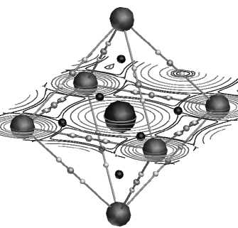
Figure 6: Octahedron with one Cl at its center and six Na at each vertex. Iso-density curves represented in the plane of Na$\cdots$Cl nearest neighbors. The six dark spheres correpond to the $(3,-1)$ CPs between Na and Cl, the twelve grey spheres to the $(3,-1)$ CPs between Cl$\cdots$Cl and the bright smallest one to the $(3,+1)$ CPs. The $(3,+3)$ CPs are not shown here.

4.2 Molecular compounds

Low densities at critical points are observed in the crystal TTF-2,5Cl₂BQ in interaction regions. Two examples are selected on table 2 and 3 respectively corresponding to the ring CP of 2,5Cl₂BQ and to the strongest hydrogen bond occuring in the plane shown in figure 7. In both cases, the smallest E${}_{\mbox{\scriptsize cutoff}}$ (50 Ry) and the largest grid spacing (0.125 a.u.) give already quite good results. These properties converge even better for all other low density CPs. As for ionic bonding, the electron density is particularly smooth close to the CPs and even smaller E${}_{\mbox{\scriptsize cutoff}}$ and $\Delta r_{\mbox{\scriptsize grid}}$ are enough. The situation is much different for covalent bonds where $\rho(\mathbf{r}_{\mbox{\scriptsize CP}})$ is much higher and the electron density varies more rapidly. All covalent bond CPs have been plotted on figure 5. Typical covalent bonds of TTF-2,5Cl₂BQ are summarized in table 4 and 5 for different E${}_{\mbox{\scriptsize cutoff}}$ and $\Delta r_{\mbox{\scriptsize grid}}$. For most bonds, the CP properties do not vary too much, except for C=O bond where low E${}_{\mbox{\scriptsize cutoff}}$ gives a value of $\nabla^{2}\rho(\mathbf{r}_{\mbox{\scriptsize CP}})$ twice as large as other E${}_{\mbox{\scriptsize cutoff}}$. This is due to the electron density that changes very rapidly along the bond path. For this reason, the C=O bond properties are also the most sensitive to $\Delta r_{\mbox{\scriptsize grid}}$ (table 5). This makes it particularly difficult to treat. Evidently, the CP characteristics of simple bonds are more easily accurate than those of double bonds.

Finally, we have checked in each case that CPs which are equivalent by symmetry are equivalent at least within the numbers of digits indicated in the different tables of this section. All these results clearly show that CPs properties can easily be deduced from densities given on regular grids, the choice of the grid stepsize depending on the nature of the bonds of interest.

5 Atomic basins

Accuracy of integration from a grid density will depend on the integration method and on the way of determining the basins surfaces but also on the accuracy of electron density data at the grid points, on the degree of missing information due to grid spacing and on the possible bias introduced by the interpolation procedure. The following residuals have been defined to estimate the accuracy of integration process: N${}_{\mbox{\scriptsize grid}}$ is the number of electrons in the unit cell obtained over all elementary volume units either by discrete summation or using analytical integral expression of the tricubic interpolation. Then $\Delta$N = N${}_{\mbox{\scriptsize grid}}$-N${}_{\mbox{\scriptsize real}}$ is the difference between the number of valence electrons obtained by integration over the whole unit cell and its expected real value. The quantities v_Ω and S_Ω respectively refer to the volume and surface of the basin $\Omega$. The number of electrons in an individual basin is denoted n_Ω. $\delta$N = $\sum\mbox{\scriptsize n}_{\Omega}$ - N${}_{\mbox{\scriptsize real}}$ is the residual after summation over all atomic basins. The basin volume uncertainty is set equal to the product of the tolerance d_tol and an estimation of the atomic surface S_Ω. The total volume uncertainty is given by $\sigma_{\mbox{\scriptsize V}}$ = $d_{tol}\,\sum\mbox{\scriptsize S}_{\Omega}$ and the residual volume error by $\Delta$V = $\sum\mbox{\scriptsize v}_{\Omega}$ - V${}_{\mbox{\scriptsize cell}}$. If the uncertainty $\sigma_{\mbox{\scriptsize V}}$ is found clearly less than the residual $\Delta$V, the question arises about the way the atomic surfaces are derived. In this case, either there are several intersections of the basin surface with one ray originating from the attractor, either the parameters used to follow the gradient path have to be modified or some attractors are missing in the input list. Finally the largest charge difference between symmetry equivalent atoms, the intra or inter molecular charge transfer (CT) and its estimated uncertainty ($\sigma_{\mbox{\scriptsize CT}}$) are the other criteria which can be used as a measure of the accuracy of the integration process.

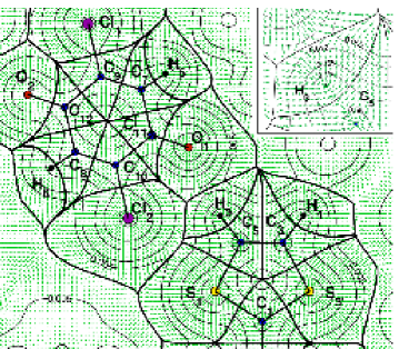
Figure 7: Representation of atomic basins in the plane containing both TTF and 2,5Cl₂BQ molecules. The strongest hydrogen bond in TTF-2,5Cl₂BQ crystal occurs between O₁ and H₃. The arrows indicate the direction and magnitude of the gradient in the plane. An example of unreachable small piece of volume due to multiple intersection of the atomic surface with a ray originating from atom C₅ can be seen on top right of the figure.

5.1 Grid spacing and ab-initio calculation convergence

In the case of NaCl, ab-initio calculations are not too sensitive to the convergence criterion E${}_{\mbox{\scriptsize cutoff}}$ so the grid spacing effect can clearly be evidenced. Well converged integration results using Romberg procedure are given in table 6. One can notice that the electron number residual $\delta$N after integration and sum over all basins is very close to $\Delta$N given as input. This residue monotonically decreases with reducing grid spacing whereas volume residual $\Delta$V is almost constant. Reasonnable estimation of interatomic charge transfer can be derived from valence density within a precision of 0.01 electron for a grid spacing of about 0.06 a.u. The prohibitive grid spacing required to get the charge transfer with the same precision from total density can be estimated to 0.03 a.u. as illustrated in figure 8.

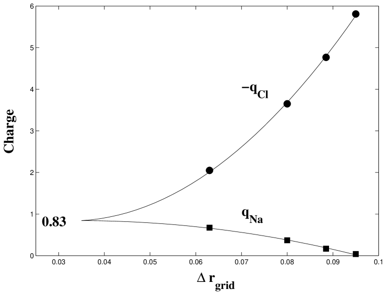
Figure 8: NaCl atomic charges from total electron density vs. grid spacing. Solid lines are guides for the eyes converging to the 0.83 charge transfer estimated from valence density.

5.2 Grid spacing and ab-initio calculations convergence

In the case of molecular crystals which exhibit short bonds with large and quickly varying electron density at their bond critical points, such C=O for example, the ab-initio calculations are more sensitive to the convergence criterion E${}_{\mbox{\scriptsize cutoff}}$ defining the plane waves expansion basis set. This is found in the integration results as illustrated in table 7 for TTF-2,5Cl₂BQ compound where the electron number residual $\delta$N after integration over all atomic basins is sligthly different from that after direct summation over the unit cell $\Delta$N. This may arise from the larger number of atoms and from the less smooth shapes of atomic basins (figure 9) in comparison to the NaCl case. Nevertheless using E${}_{\mbox{\scriptsize cutoff}}$ above 50Ry is enough to get the intermolecular charge transfer within 0.02 electron precision which is the goal that originally motivated this work.

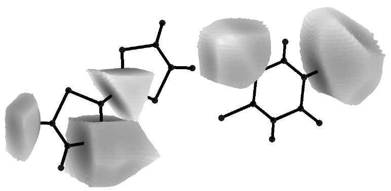
Figure 9: 3D representation of some atomic basins in the TTF-2,5Cl₂BQ charge transfer complex.

5.3 Romberg vs. fixed spherical grid integration

Different sets of parameters for the Romberg integration procedure, including adequate parameters for the basin limits search are given in table 8. Indicated CPU time corresponds to a PC machine with 800MHz processor and 512Mb RAM without including density files reading nor direct unit cell summation. The preliminary estimation of basin envelopes is done with $n_{\theta}$ = 18 and $n_{\phi}$ = 36, using a tolerance $d_{tol}$ = 0.05 a.u. This operation takes about 0.8 second per basin. The integration convergence criteria have been put only on the volume and the valence density since the grid spacing used may not correctly restore density cusps near atomic nuclei. Obtaining the intermolecular charge transfer, in the case of TTF-2,5Cl₂BQ, within a precision of about one hundredth of an electron takes about one minute per basin. The weaker criteria, although leading to unsatisfying residual from the intermolecular charge transfer point of view, nevertheless give a good indication of atomic charges within less than one second per basin. The residual volume error remains of the order of one cubic atomic unit out of nearly 2500 for the unit cell and only for the more severe integration convergence criteria may appear the problem of very precise determination of basin boundaries (figure 7, top right). The greatest discrepancy between charges obtained for equivalent atoms ranges from $10^{-4}$ for the set of parameters leading to the best integration, to $10^{-3}$ for the set giving the shorter CPU time. For comparison, integration has been done using a fixed spherical grid for all basins. The corresponding parameters and results are listed in table 9. The total number of angular loops is denoted $n_{\theta,\phi}$. Below $n_{\theta,\phi}\times n_{r}\sim 10^{4}$ integration points, no realistic atomic charges can be obtained. Indeed, the very short time that can be used with Romberg integration come from its internal $k$ order polynomial extrapolation which gives an error estimate of order $O(1/N^{2k})$ instead of $O(1/N^{2})$ for the simple discrete summation with the same number $N$ of integration points.

In the case of fixed spherical grid integration, compared to Romberg integration, the volume uncertainty is in most of the cases greater than the residual volume error, thus giving no information about missing or overlapping volumes. The discrepancy between charges of equivalent atoms is also about an order of magnitude higher. The point that makes the Romberg procedure more favorable is that the number of integration points is automatically adapted to each basin to the desired level of convergence, as illustrated for atoms C₁ and S₁ in table 8, whereas taking a fixed mean spherical grid leads to missing or biased information for some atoms and adds unnecessary points for other ones. The numbers $\overline{\mbox{\scriptsize n}}_{r}$ of radial loops indicated in table 8 are average over all angular loops for each basin.

6 Conclusion

We have shown that topological properties can be derived from electron densities given on 3D grids with tricubic interpolation to extract at any given position the density, its gradient and hessian matrix. Except for very short covalent bonds such C=0, critical points properties can be obtained with grid spacing of about 0.1 a.u. The same grid spacing can also be used to get atomic charges by integration over atomic basins with highly accurate values using the valence electron density. The integration is done with spherical coordinates system centered on the attractors and uses the robust Romberg algorithm which allows the number of integration points to be automatically adapted for each basin and offers the choice between saving computing time or giving the preference to accuracy.

Acknowledgements

This work has benefited from collaborations within the $\Psi_{k}$-ESF Research Program and the Training and Mobility of Researchers Program “Electronic Structure” (Contract: FMRX-CT98-0178) of the European Union and the Interational Joint Research Grant “Development of charge transfert materials with nanostructures” (Contract: 00MB4). Parts of the calculations have been supported by the “Centre Informatique National de l’Enseignement Supérieur” (CINES—France). We would like to thank P.E. Blöchl for his PAW code and P. Sablonniere for usefull discussions.

Table 1: Characteristics of crystalline NaCl critical points (CPs) for different grid spacing ($\Delta r_{\mbox{\scriptsize grid}}$) and numbers of plane waves (E${}_{\mbox{\scriptsize cutoff}}$). $\lambda_{1}$, $\lambda_{2}$ and $\lambda_{3}$ are the Hessian matrix eigenvalues. All values except E${}_{\mbox{\scriptsize cutoff}}$ are given in a.u.

Type	E${}_{\mbox{\scriptsize cutoff}}$	$\Delta r_{\mbox{\scriptsize grid}}$	$\rho(\mathbf{r}_{\mbox{\scriptsize CP}})$	$\nabla^{2}\rho(\mathbf{r}_{\mbox{\scriptsize CP}})$	$\lambda_{1}$, $\lambda_{2}$, $\lambda_{3}$
(3,-1)	40 Ry	0.1564	0.0130	0.0577	-0.0122, -0.0119, 0.0817
NaCl	40 Ry	0.1138	0.0130	0.0576	-0.0122, -0.0121, 0.0820
	40 Ry	0.0939	0.0130	0.0571	-0.0122, -0.0121, 0.0814
	30 Ry	0.1138	0.0130	0.0581	-0.0123, -0.0121, 0.0825
	120 Ry	0.1138	0.0130	0.0583	-0.0123, -0.0121, 0.0827
(3,-1)	40 Ry	0.1138	0.0049	0.0127	-0.0024, -0.0011, 0.0163
ClCl
(3,+1)	40 Ry	0.1138	0.0047	0.0134	-0.0025, 0.0035, 0.0124
(3,+3)	40 Ry	0.1138	0.0019	0.0056	0.0019, 0.0019, 0.0019

Table 2: Characteristics of the ring CP of 2,5Cl₂BQ and the O${}_{1}\cdots$H₃ hydrogen bond of TTF-2,5Cl₂BQ for different E${}_{\mbox{\scriptsize cutoff}}$ and $\Delta r_{\mbox{\scriptsize grid}}=0.104$ a.u.

Type	E${}_{\mbox{\scriptsize cutoff}}$	$\rho(\mathbf{r}_{\mbox{\scriptsize CP}})$	$\nabla^{2}\rho(\mathbf{r}_{\mbox{\scriptsize CP}})$	$\lambda_{1}$	$\lambda_{2}$	$\lambda_{3}$
Ring CP	50 Ry	0.0210	0.1233	-0.0128	0.0613	0.0747
2,5Cl2BQ	70 Ry	0.0209	0.1327	-0.0134	0.0664	0.0796
	90 Ry	0.0209	0.1314	-0.0131	0.0656	0.0789
	100 Ry	0.0209	0.1315	-0.0131	0.0656	0.0791
O${}_{1}\cdots$H3	50 Ry	0.0103	0.0359	-0.0106	-0.0102	0.0567
	70 Ry	0.0103	0.0384	-0.0109	-0.0103	0.0596
	90 Ry	0.0103	0.0375	-0.0108	-0.0103	0.0585
	100 Ry	0.0103	0.0370	-0.0107	-0.0103	0.0580

Table 3: Same as table 2 for different $\Delta r_{\mbox{\scriptsize grid}}$ and E${}_{\mbox{\scriptsize cutoff}}=90$ Ry.

Type	$\Delta r_{\mbox{\scriptsize grid}}$	$\rho(\mathbf{r}_{\mbox{\scriptsize CP}})$	$\nabla^{2}\rho(\mathbf{r}_{\mbox{\scriptsize CP}})$	$\lambda_{1}$	$\lambda_{2}$	$\lambda_{3}$
Cycle	0.125	0.0209	0.1314	-0.0132	0.0656	0.0790
	0.104	0.0209	0.1314	-0.0131	0.0656	0.0789
	0.085	0.0209	0.1313	-0.0131	0.0656	0.0788
O${}_{1}\cdots$H3	0.125	0.0103	0.0375	-0.0108	-0.0102	0.0585
	0.104	0.0103	0.0375	-0.0108	-0.0103	0.0585
	0.085	0.0103	0.0373	-0.0107	-0.0103	0.0584

Table 4: Characterisitcs of selected covalent bond CPs of TTF-2,5Cl₂BQ for various E${}_{\mbox{\scriptsize cutoff}}$; $\Delta r_{\mbox{\scriptsize grid}}$ = 0.104 a.u.

Type	E${}_{\mbox{\scriptsize cutoff}}$	$\rho(\mathbf{r}_{\mbox{\scriptsize CP}})$	$\nabla^{2}\rho(\mathbf{r}_{\mbox{\scriptsize CP}})$	$\lambda_{1}$	$\lambda_{2}$	$\lambda_{3}$
C11-O1	50 Ry	0.4038	0.6240	-1.0511	-0.9774	2.6526
	70 Ry	0.4070	0.3862	-1.0359	-0.9567	2.3788
	90 Ry	0.4079	0.3182	-1.0401	-0.9579	2.3162
	100 Ry	0.4079	0.3131	-1.0394	-0.9571	2.3096
C6-S2	50 Ry	0.2089	-0.3931	-0.3364	-0.2823	0.2256
	70 Ry	0.2094	-0.4185	-0.3370	-0.2835	0.2021
	90 Ry	0.2094	-0.4243	-0.3371	-0.2833	0.1961
	100 Ry	0.2094	-0.4251	-0.3371	-0.2833	0.1954
C1-C2	50 Ry	0.3410	-1.2044	-0.7568	-0.5956	0.1480
	70 Ry	0.3387	-1.0740	-0.7496	-0.5893	0.2649
	90 Ry	0.3388	-1.0786	-0.7453	-0.5853	0.2519
	100 Ry	0.3387	-1.0734	-0.7452	-0.5852	0.2570

Table 5: Same as table 4 for different $\Delta r_{\mbox{\scriptsize grid}}$; E${}_{\mbox{\scriptsize cutoff}}$=90 Ry.

Type	$\Delta r_{\mbox{\scriptsize grid}}$	$\rho(\mathbf{r}_{\mbox{\scriptsize CP}})$	$\nabla^{2}\rho(\mathbf{r}_{\mbox{\scriptsize CP}})$	$\lambda_{1}$	$\lambda_{2}$	$\lambda_{3}$
C11-O1	0.125	0.4080	0.2268	-1.0899	-1.0180	2.3347
	0.104	0.4079	0.3182	-1.0401	-0.9579	2.3162
	0.085	0.4079	0.2913	-1.0266	-0.9879	2.3058
C6-S2	0.125	0.2095	-0.4207	-0.3353	-0.2824	0.1970
	0.104	0.2094	-0.4243	-0.3371	-0.2833	0.1961
	0.085	0.2095	-0.4239	-0.3369	-0.2835	0.1965
C1-C2	0.125	0.3388	-1.0770	-0.7438	-0.5841	0.2509
	0.104	0.3388	-1.0786	-0.7453	-0.5853	0.2519
	0.085	0.3388	-1.0804	-0.7462	-0.5862	0.2520

Table 6: NaCl integration results vs. $\Delta r_{\mbox{\scriptsize grid}}$; E${}_{\mbox{\scriptsize cutoff}}$=120 Ry.

$\Delta r_{\mbox{\scriptsize grid}}$	0.095	0.0885	0.08	0.063
$\Delta$N	0.0362	0.0289	0.0198	0.0086
$\delta$N	0.0367	0.0285	0.0199	0.0090
$\Delta$V	0.095	0.096	0.020	0.090
q${}_{\mbox{\scriptsize Na}}$	0.8282	0.8282	0.8188	0.8283
v${}_{\mbox{\scriptsize Na}}$	63.36	63.36	63.29	63.36
q${}_{\mbox{\scriptsize Cl}}$	-0.8648	-0.8572	-0.8387	-0.8373
v${}_{\mbox{\scriptsize Cl}}$	236.18	236.18	236.17	236.17
CT	0.85	0.84	0.83	0.83
$\sigma_{\mbox{\scriptsize CT}}$	0.04	0.03	0.02	0.01

Table 7: TTF-2,5Cl₂BQ integration results vs. E${}_{\mbox{\scriptsize cutoff}}$ ( $\Delta r_{\mbox{\scriptsize grid}}$ = 0.104 a.u.);.

E${}_{\mbox{\scriptsize cutoff}}$ (Ry)	50	70	90	100
$\Delta$N	-0.006	-0.005	-0.006	-0.006
$\delta$N	0.066	0.022	0.020	0.020
$\Delta$V	-0.92	-1.44	-1.93	-1.89
q${}_{\mbox{\scriptsize TTF}}$	0.455	0.453	0.452	0.453
q${}_{\mbox{\scriptsize 2,5Cl${}_{2}$BQ}}$	-0.522	-0.475	-0.472	-0.473
CT	0.49	0.46	0.46	0.46
$\sigma_{\mbox{\scriptsize CT}}$	0.07	0.02	0.02	0.02

Table 8: Sets of tested parameters and results for Romberg integration on the charge transfer crystal TTF-2,5Cl₂BQ. The cell volume is V${}_{\mbox{\scriptsize cell}}$ = 2493.062 a.u. Direct integration of valence electron density over the whole unit cell gives an input error $\Delta$ N = -0.0056 electron. $\Delta r_{\mbox{\scriptsize grid}}$ = 0.104 a.u; E${}_{\mbox{\scriptsize cutoff}}$ = 90 Ry

Basin search
$dr_{o}=d_{tol}$	5 10-2	5 10-3	10-3	5 10-4	5 10-4	10-4
A	5	50	250	500	500	2500
B	0.5	0.5	0.5	1	1	1
Romberg
$k_{min}$	4	6	6	6	6	6
$\epsilon_{r}$	10-3	10-3	5 10-4	10-4	2 10-7	10-7
$\epsilon_{\phi}$	10-2	10-2	5 10-3	10-3	8 10-5	10-5
$\epsilon_{\theta}$	5 10-2	5 10-2	10-2	10-3	5 10-5	10-4
CPU time	23s	104s	222s	19min.	3.5h	43h
$\delta$N	-0.413	0.080	0.056	0.019	0.014	0.006
$\Delta$V	18.98	-1.88	-0.98	-1.56	-0.77	-1.11
$\sigma_{\mbox{\scriptsize V}}$	120	12	2.4	1.25	1.2	0.2
q${}_{\mbox{\scriptsize TTF}}$	0.862	0.424	0.434	0.448	0.454	0.455
q${}_{\mbox{\scriptsize 2,5Cl${}_{2}$BQ}}$	-0.448	-0.503	-0.490	-0.467	-0.468	-0.461
CT	0.65	0.46	0.46	0.46	0.461	0.458
$\sigma_{\mbox{\scriptsize CT}}$	0.40	0.08	0.06	0.02	0.015	0.006
C1
$n_{\theta,\phi}$	89	1089	1089	1441	8639	38081
$\overline{\mbox{\scriptsize n}}_{r}$	15	33	33	56	212	258
q	-0.311	-0.285	-0.285	-0.283	-0.284	-0.284
v	69.11	65.96	65.96	65.50	65.56	65.56
S1
$n_{\theta,\phi}$	81	1089	1089	1089	2591	8513
$\overline{\mbox{\scriptsize n}}_{r}$	23	33	40	61	292	373
q	0.249	0.252	0.255	0.258	0.258	0.258
v	183.22	181.86	181.84	181.95	182.21	182.18

Table 9: Sets of tested parameters and results for fixed spherical grid integration on TTF-2,5Cl₂BQ compound.

Basin search
$dr_{o}=d_{tol}$	5 10-3	5 10-3	5 10-4	5 10-4
A	50	50	500	500
B	0.5	0.5	0.5	1
Spherical Grid
$n_{\theta}$	18	30	50	72
$n_{\theta,\phi}$	406	1134	3162	6574
$n_{r}$	30	50	100	240
CPU time	53s	135s	20min.	2.2h
$\delta$Ntot	1.534	-0.192	-0.204	-0.227
$\delta$Nval	0.147	0.061	0.041	0.025
$\Delta$V	-30.50	-2.18	-0.27	-0.35
$\sigma_{\mbox{\scriptsize CT}}$	12.5	11	1.2	1.2
q${}_{\mbox{\scriptsize TTF}}$	0.398	0.433	0.442	0.449
q${}_{\mbox{\scriptsize 2,5Cl${}_{2}$BQ}}$	-0.545	-0.494	-0.484	-0.474
CT	0.47	0.46	0.46	0.46
$\sigma_{\mbox{\scriptsize CT}}$	0.15	0.06	0.04	0.03
C1
q	-0.286	-0.284	-0.285	-0.284
v	65.14	65.52	65.59	65.55
S1
q	0.251	0.254	0.256	0.257
v	181.96	182.21	182.20	182.23