QED theory of transition probabilities and line profiles in highly charged ions

Abstract

A rigorous QED theory of the spectral line profiles is applied to transition probabilities in few-electron highly charged ions. Interelectron interaction corrections are included as well as radiative corrections. Parity nonconserving (PNC) amplitudes with effective weak interactions between the electrons and nucleus are also considered. QED and interelectron interaction corrections to the PNC amplitudes are derived.

Key words: QED corrections, line profile, Lamb shift, highly-charged ions, few-electron systems, parity nonconservation
PACS: 31.30.Jv, 12.20.Ds, 31.15.-p, 31.10.+z, 11.30.Er, 12.20.-m

, , , , , and

1 Introduction

The spectra of the highly charged ions (HCI) are currently under intensive experimental investigations [1] - [2]. Due to the strong field of the nucleus acting on the electrons in HCI, the relevant theory should be fully relativistic and based on the principles of QED. Up to now major experimental and theoretical efforts were concentrated on the evaluation of the energy level shifts due to radiative effects (Lamb shift) or to the interelectron interaction, on the hyperfine splitting and on the bound electron g-factor. The recent status of the problem was described in a series of books and reviews [3], [4], [5], [6].

Transition probabilities were studied less intensively, though a considerable amount of experimental [7] - [8] and theoretical  [9] - [10] investigations also exists. The full QED theory for the transition probabilities was considered in  [3], [11] on the basis of the S-matrix approach and in [12] employing the two-time Green function approach (see also [6]).

In this paper we apply the most general QED line profile approach to the derivation of expressions for transitions probabilities in HCI with radiative, interelectron interactions and weak interaction corrections.

The problem of the natural line profile in atomic physics was considered first in terms of quantum mechanics by Weisskopf and Wigner [13]. In terms of modern QED it was first formulated for one-electron atoms by Low [14]. In [14] the appearance of the Lorentz profile in the resonance approximation within the framework of QED was described and the nonresonant corrections were estimated. Later the line profile QED theory was modified also for few-electron ions  [15] (see also  [16],  [3]) and applied to the theory of overlapping resonances in two-electron HCI  [17], [18]. Another application was provided to the theory of nonresonant corrections in HCI and in neutral hydrogen  [19], [20], [21].

It was found in [22] that the line profile approach provides a convenient tool for calculating energy corrections. The most natural way to calculate the energy shift in QED is to calculate the resonance shift in some scattering process. This way clearly indicates the limits up to which the concept of the energy of an exited states has a physical meaning – that is the resonance approximation. The exact theoretical value for the energy of the exited state defined, for example, by the Green function pole, can be compared directly with the measurable quantities only in the resonance approximation when the line profile is described by the two parameters: energy E and width $\Gamma$. Beyond this approximation the evaluation of E and $\Gamma$ should be replaced by the evaluation of the line profile for the particular process. For applications of the line profile approach to the calculation of energy level corrections see  [23], [24].

In [15], [16] the line profile theory in QED was developed on the basis of the evolution operator $\hat{S}(0,\infty)$. Such a consideration, though most natural for describing spontaneous emission and absorption processes, faces serious difficulties due to unrenormalizability of the corresponding S-matrix elements $<f|\hat{S}(0,\infty)|i>$. The resonance approximation itself yields correct results  [15], [16], but the introduction of radiative corrections leads to the appearance of unrenormalizable expressions.

Therefore in this paper we will use only renormalizable ”full” S-matrix elements $<f|\hat{S}(\infty,-\infty)|i>$.

During the last decades the parity nonconservation (PNC) processes in HCI became a topic of permanent interest (up to now only from a theoretical point of view) [25] -  [31], [32].

In neutral atoms, where successful experiments and accurate theoretical calculations were performed, the main uncertainty is introduced by electron correlation effects arising due to the complicated atomic structure. In few-electron HCI electron correlation does not play any significant role what greatly simplifies the theoretical treatment. The major corrections to PNC matrix elements in HCI are the radiative ones. This allows, in principle, to test the Standard Model of electroweak interactions beyond the ”tree” level. It is especially important that the experiments with HCI would provide these tests in the presence of strong fields.

Partly the electroweak radiative corrections in HCI were calculated in Ref. [32]. In this work we present the full treatment of the QED part of the electroweak corrections based on the line profile approach. According to [32] these corrections are dominant in HCI and, unlike the so called ”oblique” corrections, are strongly field-dependent, i.e. different in HCI and neutral atoms.

The paper is organized as follows. In section 2 we begin with the description of the process of resonant photon scattering on the ”tree” level. In section 3 electron self-energy insertions (SE) in the electron propagator within the resonance approximation are considered. It is shown that they improve the energy denominator of the photon emission (absorption) amplitude. The same is done for the vacuum polarization (VP) insertions. In section 4 the standard expressions for the Lorentz line profile in the case of the photon emission (absorption) process is derived; in section 5 it is shown in which way higher-order radiative corrections to the energy can be incorporated in the Lorentz denominator. Section 6 is devoted to the derivation of radiative (QED) corrections to the initial state in the photon emission amplitude.

The derivation of QED corrections to the final state requires more refined considerations, that are contained in Section 7. Here the process of double resonance photon scattering is introduced. In sections 8, 9 the SE and VP insertions in the different electron propagators in the Feynman diagram describing the double photon scattering are considered. These insertions produce energy shifts to both resonant energy denominators of the two-photon emission amplitude. In section 10 the Lorentz profile for the one-photon emission process in the case of an unstable finite state is derived from the two-photon emission amplitude. This derivation includes the integration over the frequency of one of the photons. The resulting expressions can also be used to include the Lamb shift of the final state in the one-photon Lorentz denominator. The width of the final ground state formally can be set equal to zero; this approach can be considered as a kind of regularization of the singular amplitudes. Section 11 is devoted to the derivation of QED corrections to the photon emission amplitude (final state).

In section 12 the vertex correction to the photon emission amplitude is evaluated; it is shown, that the ultraviolet and infrared divergencies, contained in the vertex cancel with the corresponding divergencies in the so called ”derivative” corrections.

QED corrections to the amplitude admixed by the effective PNC weak potential are investigated in Sections 13-15. It is supposed that the mixed states with opposite parity are separated only by the Lamb shift and it is shown how the vanishing denominators in the approximation of noninteracting electrons acquire a nonvanishing value. The cancellation of the divergencies in the vertex and derivative graphs with the effective PNC potential is also demonstrated.

In sections 16-19 the results obtained earlier are generalized to few-electron ions. The first-order interelectron interaction is taken into account explicitly. The introduction of higher-order interelectron interaction corrections is discussed. First-order interelectron interaction corrections to the PNC amplitude in the two-electron HCI are derived. Section 20 presents a short summary of all the results obtained in preceeding sections.

2 Resonant scattering of a photon on an atomic electron

In this section we consider first the process of elastic photon scattering on an atomic electron in lowest-order QED perturbation theory. As usual for bound-electron QED we employ the Furry picture in which the electrons are described by the solution of the Dirac equation

$$(p\!\!\!/-m+\gamma_{0}eV)\Psi=0\,.$$ (1)

Here $p\!\!/\equiv\gamma_{\mu}p^{\mu},p^{k}\equiv-i\nabla(k=1,2,3),p_{0}=E$, where $m$ and $e$ are the electron mass and charge, respectively, $E$ is the energy, $\gamma_{\mu}$ are the Dirac matrices and $V$ is the potential of the nucleus (point-like or extended). The pseudoeuclidean metric (+ - - -) in 4-space is used. We employ relativistic units $\hbar=c=1$ throughout the paper. The Feynman graph corresponding to the process under consideration is presented in Fig. 1. We will consider the elastic scattering and will assume that the initial (final) state $A$ is the ground state. According to the standard correspondence rules (see, for example, [3]) the S-matrix element for the graph Fig. 1 is:

$$S^{(2)}=e^{2}\int d^{4}x_{1}d^{4}x_{2}\bar{\Psi}_{A}(x_{1})\gamma_{\mu_{1}}A_{\omega}^{\mu_{1}*}S(x_{1},x_{2})\gamma_{\mu_{2}}A^{\mu_{2}}_{\omega^{\prime}}(x_{2})\Psi_{A}(x_{2})\,,$$ (2)

where $\Psi_{A}(x)=\Psi_{A}(\vec{x}\,)e^{-iE_{A}t}$ is the electron wave function, $\bar{\Psi}_{A}$ is the Dirac conjugated wave function, $A_{\omega}^{\mu_{1}*}(x)=A_{\omega}^{\mu_{1}*}(\vec{x})\,e^{-i\omega t}$ is the wave function (electromagnetic potential) for an absorbed photon with frequency $\omega$. The electron propagator for bound electrons is taken in the form:

$$S(x_{1},x_{2})=\frac{1}{2\pi i}\int\limits_{-\infty}^{\infty}e^{i\omega_{1}(t_{1}-t_{2})}\sum_{n}\frac{\bar{\Psi}_{n}(\vec{x}_{1})\Psi_{n}(\vec{x}_{2})}{E_{n}(1-i0)+\omega_{1}}d\omega_{1}\,,$$ (3)

where the sum runs over the whole Dirac spectrum. Integrating over time and frequency variables $t_{1},t_{2},\omega_{1}$ and using the relation between the S-matrix and the amplitude $U$

$$S_{if}=-2\pi i\,\delta(E_{i}-E_{f})U_{if}$$ (4)

we will obtain for the scattering amplitude

$$U^{(2)}_{\rm sc}=\sum_{n}\frac{(U^{*}_{\omega})_{An_{1}}(U_{\omega^{\prime}})_{n_{1}A}}{E_{n_{1}}-E_{A}-\omega}$$ (5)

with the condition $\omega=\omega^{\prime}$, which implies energy conservation. Here we abbreviate

$$U_{\omega}(\vec{x})\equiv e\gamma_{\mu}A^{\mu}_{\omega}(\vec{x})\,.$$ (6)

In the resonance approximation the photon frequency $\omega$ is close to the energy difference of two atomic levels: $\omega\approx E_{A^{\prime}}-E_{A}$. Accordingly, we have to retain only one term in the sum over $n$ in Eq. (5)

$$U^{(2)\rm{res}}_{\rm{sc}}=\frac{(U^{*}_{\omega})_{AA^{\prime}}(U_{\omega^{\prime}})_{A^{\prime}A}}{E_{A^{\prime}}-E_{A}-\omega}\,.$$ (7)

Eq. (7) shows that in the resonance approximation the scattering amplitude factorizes into an emission and an absorption part. It follows from Eq. (6) that the emission amplitude can be expressed as

$$U_{\rm{em}}=\frac{(U^{*}_{\omega})_{AA^{\prime}}}{E_{A^{\prime}}-E_{A}-\omega}\,.$$ (8)

For the absorption we may write

$$U_{\rm{ab}}=\frac{(U_{\omega^{\prime}})_{A^{\prime}A}}{E_{A^{\prime}}-E_{A}-\omega^{\prime}}\,.$$ (9)

This implies that the Lorentz profiles for emission and for absorption will be identical as it should be. Eq. (7) also indicates the limit, up to which the absorption and emission processes are independent - that is the resonance approximation. Only within the resonance approximation the spontaneous emission rate is independent from the process how the exited state is prepared.

This approximation is quite adequate in atomic physics. Nonresonant corrections to the transition frequencies are still too small to be observed in present modern experiments [19] - [21].

3 Radiative insertions in the electron propagator

In this section we consider radiative insertions in the electron propagator. The electron self-energy insertion is depicted in Fig. 2. The S-matrix element corresponding to this diagram can be expressed as

$$S^{4}=e^{4}\int d^{4}x_{1}\ldots d^{4}x_{4}\,\bar{\Psi}_{A}(x_{1})\gamma_{\mu_{1}}A^{\mu_{1}\ast}_{\omega}(x_{1})S(x_{1},x_{2})\\ \times\gamma_{\mu_{2}}S(x_{2},x_{3})\gamma_{\mu_{3}}D^{\mu_{2}\mu_{3}}(x_{2},x_{3})S(x_{3},x_{4})\gamma_{\mu_{4}}A^{\mu_{4}}_{\omega^{\prime}}(x_{4})\Psi_{A}(x_{4})\,,$$ (10)

where $D^{\mu_{1}\mu_{2}}(x_{1},x_{2})$ denotes the photon propagator in Feynman gauge

$$D^{\mu_{1}\mu_{2}}(x_{1},x_{2})=\frac{1}{2\pi i}\frac{\delta^{\mu_{1}\mu_{2}}}{r_{12}}\int\limits_{-\infty}^{\infty}d\omega\,e^{i\omega(t_{1}-t_{2})+i|\omega|r_{12}}$$ (11)

with $r_{12}=|\vec{x}_{1}-\vec{x}_{2}|$. Integrating over time and frequency variables and using again Eq. (4), we obtain the following expression for the correction to the scattering amplitude

$$U^{(4)}_{\rm sc}=-\sum_{n_{1},n_{3}}\frac{(U^{*}_{\omega})_{An_{1}}(\hat{\Sigma}(E_{A}+\omega))_{n_{1}n_{3}}(U_{\omega^{\prime}})_{n_{3}A}}{(E_{n_{1}}-E_{A}-\omega)(E_{n_{3}}-E_{A}-\omega)}\,,$$ (12)

where $\hat{\Sigma}(E)$ is the electron self-energy operator defined by its matrix elements

$$(\hat{\Sigma}(E))_{n_{1}n_{3}}=\frac{e^{2}}{2\pi i}\sum_{n_{2}}\left(\frac{\gamma_{\mu_{1}}\gamma^{\mu_{2}}}{r_{12}}I_{E_{n_{2}}-E}(r_{12})\right)_{n_{1}n_{2}n_{2}n_{3}}\,,$$ (13)

together with

$$I_{E_{n_{2}}-E}(r_{12})=-\int\limits_{-\infty}^{\infty}\frac{d\omega\,e^{i|\omega|r_{12}}}{E_{n_{2}}-E+\omega}\,.$$ (14)

In the resonance approximation we have $n_{1}=n_{3}=A^{\prime}$ and the correction to the scattering amplitude takes the form

$$U^{(4)\rm{res}}_{\rm{sc}}=-U^{(2)\rm{res}}_{\rm{sc}}\,\frac{(\hat{\Sigma}(E_{A}+\omega))_{A^{\prime}A^{\prime}}}{(E_{A^{\prime}}-E_{A}-\omega)}\,.$$ (15)

Repeating the insertions in the resonance approximation (the next term of this series is shown in Fig. 3) leads to a geometric progression. Resummation of this progression yields [14]

$$U^{\rm{res}}_{\rm{sc}}=\frac{(U^{*}_{\omega})_{AA^{\prime}}(U_{\omega^{\prime}})_{A^{\prime}A}}{(\tilde{E}_{A^{\prime}}-E_{A}-\omega)}\,,$$ (16)

where

$$\tilde{E}_{A^{\prime}}=E_{A}+(\hat{\Sigma}(E_{A}+\omega))_{A^{\prime}A^{\prime}}\,.$$ (17)

Accordingly, in the resonance approximation the emission amplitude is represented by the expression

$$U_{\rm{em}}=\frac{(U^{*}_{\omega})_{AA^{\prime}}}{\tilde{E_{A^{\prime}}}-E_{A}-\omega}\,.$$ (18)

The operator $\hat{\Sigma}(E_{A}+\omega)$ may be expanded into a Taylor series around the value $E_{A}+\omega=E_{A^{\prime}}$:

$$\hat{\Sigma}(E_{A}+\omega)=\hat{\Sigma}(E_{A^{\prime}})+(E_{A^{\prime}}-E_{A}-\omega)\Sigma^{\prime}(E_{A^{\prime}})+\ldots\,,$$ (19)

where $\Sigma^{\prime}(E_{A^{\prime}})\equiv(\frac{\partial\hat{\Sigma}(E)}{\partial E})_{E=E_{A^{\prime}}}$. The first two terms of the expansion (19) are ultraviolet divergent and have to be renormalized. The renormalization of the first term to all orders in $\alpha Z$ is well known. A commonly employed covariant procedure has been developed by Mohr  [33] (see further developments in  [4]). Within this approach the divergencies are canceled analytically. Originally Mohr’s method was first applicable numerically to high and intermediate $Z$ values, but recently the high accurate extension for $Z=1$ was also carried out [34]. Another noncovariant approach is based on the partial wave expansion of $\hat{\Sigma}$ together with a numerical cancellation of divergencies for each partial wave has been proposed in [35], [36]. This approach is known as partial wave renormalization (PWR). A variant of the PWR where the divergencies are canceled partly analytically and partly numerically utilizes the multicommutator expansion method  [37], [38].

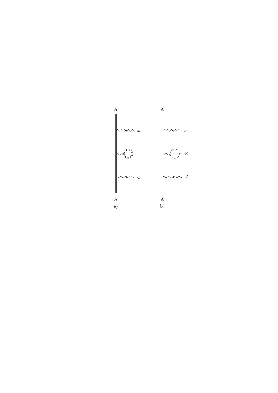
Figure 4: Vacuum polarization insertions in the electron propagator. Part a) corresponds to the exact expression and part b) describes the Uehling approximation. The ordinary solid line in Fig. 4b denotes the free electron propagation, the dashed line with the cross at the end denotes the interaction with the nuclear potential.

Apart from self energy (SE) also the vacuum-polarization (VP) insertions in the electron propagator of Fig. 1 should be considered to all orders in resonance approximation. The lowest order VP insertion is depicted in Fig. 4a. For the VP correction the Uehling approximation is frequently applied. In this approximation the bound-electron propagator in the VP loop (Fig. 4a) is expanded in powers of the nuclear potential ( in powers of $\alpha Z$) and only the first term of the expansion is retained (Fig. 4b). The Uehling approximation leads already to fairly good results even for high $Z$ values [4]. We will adopt this approximation in our derivations for simplicity. Accordingly, the VP insertions leads to the following modification of Eq. (17):

$$\tilde{E}_{A^{\prime}}=E_{A}+(\hat{\Sigma}(E_{A}+\omega))_{A^{\prime}A^{\prime}}+(V_{U})_{A^{\prime}A^{\prime}}\,,$$ (20)

where $V_{U}$ is the Uehling potential [39].

4 Line profile for the emission process

In order to obtain the line profile for the emission process we retain the first term of the Taylor expansion (19) and consider the energy denominator in Eq. (18) with a shifted energy value

$$\tilde{E}_{A^{\prime}}=E_{A^{\prime}}+(\hat{\Sigma}(E_{A^{\prime}}))_{A^{\prime}A^{\prime}}+(V_{U})_{A^{\prime}A^{\prime}}\,,$$ (21)

where

$$(\hat{\Sigma}(E_{A^{\prime}}))_{A^{\prime}A^{\prime}}=L^{\rm SE}_{A^{\prime}}-\frac{i}{2}\Gamma_{A^{\prime}}\,.$$ (22)

$L^{\rm SE}_{A^{\prime}}$ denotes the lowest-order electron self-energy contribution to the Lamb shift and $\Gamma_{A^{\prime}}$ denotes the lowest order radiative width. The other lowest-order correction to the Lamb shift is the vacuum polarization

$$(V_{U})_{A^{\prime}A^{\prime}}=L^{\rm VP}_{A^{\prime}}\,.$$ (23)

Since the corresponding energy shift is real the vacuum polarization does not contribute to the width. To this approximation the emission amplitude reads

$$U_{\rm{em}}=\frac{(U_{\omega}^{*})_{AA^{\prime}}}{E_{A^{\prime}}+L_{A^{\prime}}-E_{A}-\omega-\frac{i}{2}\Gamma_{A^{\prime}}}\,,$$ (24)

where $L_{A^{\prime}}=L_{A^{\prime}}^{{\rm SE}}+L^{{\rm VP}}_{A^{\prime}}$. A method to incorporate the Lamb shift and the finite width of the state $A$ in the energy denominator of Eq. (24) will be discussed below in section  10.

As the next steps of the calculation we have to take the square modulus of $U_{\rm{em}}$ and to integrate over the emission directions $\vec{\nu}$ of the photon and to sum over the polarizations $\vec{e}$. Taking into account the definition

$$\omega^{2}_{\rm{res}}\sum_{\vec{e}}\int d\vec{\nu}\,|(U^{*}_{\omega})_{AA^{\prime}}|^{2}=\Gamma_{AA^{\prime}}\,,$$ (25)

where $\omega_{\rm{res}}$ is the resonant photon frequency, $\Gamma_{AA^{\prime}}$ is the partial width of the level $A^{\prime}$, associated with the transition $A^{\prime}\rightarrow A$, we obtain an expression for the transition probability $dW_{AA^{\prime}}(\omega)$ for the emission process

$$dW_{AA^{\prime}}(\omega) = \frac{1}{2\pi}\sum_{\vec{e}}\int d\vec{\nu}\,|U_{\rm{em}}|^{2}\omega^{2}d\omega$$ (26)

$$= \frac{1}{2\pi}\frac{\Gamma_{AA^{\prime}}d\omega}{(E_{A^{\prime}}+L_{A^{\prime}}-E_{A}-\omega)^{2}+\frac{1}{4}\Gamma^{2}_{A^{\prime}}}\,.$$

Eq. (26) defines the Lorentz profile for the emission spectral line. The values for the resonance frequency in zeroth-order and in first-order approximation read:

$$\omega^{0}_{\rm{res}} =E_{A^{\prime}}-E_{A},$$ (27)

$$\omega^{1}_{\rm{res}} =E_{A^{\prime}}+L_{A^{\prime}}-E_{A}\,.$$ (28)

For further derivations it is more convenient to introduce a complex resonance frequency

$$\omega^{1}_{\rm{res}}=E_{A^{\prime}}+(\hat{\Sigma}(E_{A^{\prime}}))_{A^{\prime}A^{\prime}}-E_{A}\,.$$ (29)

5 Higher-order radiative corrections to the energy

In this section we explain how to incorporate higher-order corrections to the energy levels in the denominator of Eq. (26). First, we have to take into account the next term of the Taylor expansion (19). Considering this term as a correction to the energy denominator, we have to insert the resonance frequency given by Eq. (29). This leads to the ”reducible” part of the second-order loop-after-loop self-energy (SESE) correction [3], [40].

$$\triangle E_{A^{\prime}}({\rm SESE,lal,red})=(\hat{\Sigma}(E_{A^{\prime}}))_{A^{\prime}A^{\prime}}(\hat{\Sigma}^{\prime}(E_{A^{\prime}}))_{A^{\prime}A^{\prime}}\,.$$ (30)

The irreducible part of the SESE loop-after-loop correction can be obtained according to Fig. 3, where $n_{2}\neq A^{\prime}$. The corresponding contribution to the scattering amplitude is given by

$$U^{(6)}_{\rm se}=-\frac{(U^{*}_{\omega})_{AA^{\prime}}}{E_{A^{\prime}}-E_{A}-\omega}\sum_{n_{2}\neq A^{\prime}}\frac{(\hat{\Sigma}(E_{A}+\omega))_{A^{\prime}n_{2}}(\hat{\Sigma}(E_{A}+\omega))_{n_{2}A^{\prime}}}{E_{n_{2}}-E_{A}-\omega}\\ \times\frac{1}{E_{A^{\prime}}-E_{A}-\omega}(U_{\omega})_{A^{\prime}A}\,.$$ (31)

In the sum over $n_{2}\neq A^{\prime}$ we can set $E_{A}+\omega=E_{A^{\prime}}$. This sum can be viewed as a complicated higher-order insertion in the electron propagator in Fig. 1. Repeating this insertion subsequently in the resonance approximation, we finally obtain the additional energy shift of the denominator of the emission amplitude in Eq. (18). This shift represents the irreducible loop-after-loop SESE correction to the energy of the level $A^{\prime}$:

$$\triangle E_{A^{\prime}}({\rm SESE,lal,irr})=\sum_{n_{2}\neq A^{\prime}}\frac{({\hat{\Sigma}}(E_{A^{\prime}}))_{A^{\prime}n_{2}}({\hat{\Sigma}}(E_{A^{\prime}}))_{n_{2}A^{\prime}}}{E_{n_{2}}-E_{A^{\prime}}}\,.$$ (32)

The corrections (31) and (32) represent only two of the second-order radiative corrections to the energy. The full set of these corrections, i.e. the remaining second-order self-energy (SESE) corrections, the second-order vacuum polarization (VPVP) and the mixed SEVP corrections can be included in the denominator of Eq. (18) and hence in Eq. (26) in the same way. The expressions for these corrections can be found in [4] and  [40], respectively.

6 Radiative corrections to the emission amplitude (initial state)

SE corrections to the amplitude (initial state), i.e. the SE correction to the wave function $A^{\prime}$ in the expression for the amplitude follows according to the diagram in Fig. 2 for intermediate states $n_{1}\neq A^{\prime}$. In this case the correction to $U_{\rm{sc}}$ takes the form

$$U_{\rm{sc}}^{(4)}=-\sum_{n_{1}\neq A^{\prime}}\frac{(U^{*}_{\omega})_{An_{1}}(\hat{\Sigma}(E_{A}+\omega))_{n_{1}A^{\prime}}}{E_{n_{1}}-E_{A}+\omega}\,\frac{(U_{\omega})_{A^{\prime}A}}{E_{A^{\prime}}-E_{A}-\omega}\,.$$ (33)

Here in the sum over $n_{1}$ we can set $E_{A}+\omega=E_{A^{\prime}}$. Comparing the expression  (33) with Eqs. (7) and  (8) we observe, that Eq. (33) represents the corrections to the matrix element $(U^{*}_{\omega})_{AA^{\prime}}$ in the emission amplitude. Assuming, that all the improvements (corrections to the energy of the level $A^{\prime}$) in the denominator are already performed, we now can rewrite formula (18) in the form

$$U_{\rm{em}}=\frac{(U^{*}_{\omega})_{A\tilde{A}^{\prime}}}{\tilde{E_{A^{\prime}}}-E_{A}-\omega}\,,$$ (34)

where

$$(U^{*}_{\omega})_{A\tilde{A}^{\prime}}=\sum_{n_{1}\neq A^{\prime}}\frac{(U^{*}_{\omega})_{An_{1}}(\hat{\Sigma}(E_{A^{\prime}}))_{n_{1}A^{\prime}}}{E_{n_{1}}-E_{A^{\prime}}}\,.$$ (35)

The vacuum-polarization contribution can be introduced immediately into Eq. (35)

$$(U^{*}_{\omega})_{A\tilde{A}^{\prime}}=\sum_{n_{1}\neq A^{\prime}}\frac{(U^{*}_{\omega})_{An_{1}}[(\hat{\Sigma}(E_{A^{\prime}}))_{n_{1}A^{\prime}}+(V_{U})_{n_{1}A^{\prime}}]}{E_{n_{1}}-E_{A^{\prime}}}\,.$$ (36)

In order to obtain the correction to the state $A$ in the matrix element $(U^{*}_{\omega})_{AA^{\prime}}$ as well as the correction to the energy $E_{A}$ in the denominator of Eq. (34), we have to consider the diagrams with radiative insertions in the upper external electron line. However, these graphs appear to be divergent. The singularity occurring can not be regularized in a direct manner. To avoid this technical difficulty we may consider the double-photon-resonance scattering process of an electron in the state $A_{0}$ with resonance absorption into the state $A$ and finally into the state $A^{\prime}$. If $A$ is the ground state, $A_{0}$ is some fictitious state that plays the role of a regulator. However the final expression for the line profile for the emission transition probability $A^{\prime}\rightarrow A$ does not depend on $A_{0}$ and contains only a dependence on the width $\Gamma_{A}$ of the state $A$. This width can be set equal to zero at the end of the evaluations. Such a regularization program will be carried out in the following sections.

7 Double resonant photon scattering

According to the idea discussed at the end of the previous section, we now have to consider the process depicted in the Feynman diagram of Fig. 5. After the integration over time and frequency variables the scattering amplitude corresponding to the process depicted in Fig. 5 takes the form

$$U^{(4)}_{\rm{sc}}=\sum_{n_{1}}\frac{(U^{*}_{\omega_{0}})_{A_{0}n_{1}}}{E_{n_{1}}-E_{A_{0}}-\omega_{0}}\sum_{n_{2}}\frac{(U^{*}_{\omega})_{n_{1}n_{2}}}{E_{n_{2}}-E_{A_{0}}-\omega_{0}-\omega}\\ \times\sum_{n_{3}}\frac{(U_{\omega^{\prime}})_{n_{2}n_{3}}(U_{\omega_{0}^{\prime}})_{n_{3}A_{0}}}{E_{n_{3}}-E_{A_{0}}-\omega_{0}-\omega+\omega^{\prime}}\,.$$ (37)

The energy conservation during this process is implemented by the condition

$$\omega_{0}+\omega=\omega^{\prime}+\omega_{0}^{\prime}$$ (38)

and the resonance frequencies are given by

$$\omega_{0}=\omega_{0^{\prime}}=E_{A}-E_{A_{0}}\,,$$ (39)

$$\omega=\omega^{\prime}=E_{A^{\prime}}-E_{A}\,.$$ (40)

In the resonance case we have to set $n_{1}=A$, $n_{2}=A^{\prime}$, $n_{3}=A$ in Eq. (37), which yields

$$U^{(4)\rm{res}}_{\rm{sc}}=\frac{(U^{*}_{\omega_{0}})_{A_{0}A}(U^{*}_{\omega})_{AA^{\prime}}(U_{\omega^{\prime}})_{A^{\prime}A}(U_{\omega_{0}^{\prime}})_{AA_{0}}}{(E_{A}-E_{A_{0}}-\omega_{0})(E_{A^{\prime}}-E_{A_{0}}-\omega_{0}-\omega)(E_{A}-E_{A_{0}}-\omega_{0}^{\prime})}\,.$$ (41)

In order to describe the line profile for double-photon emission we have to consider

$$U_{\rm em}=\frac{(U^{*}_{\omega_{0}})_{A_{0}A}(U^{*}_{\omega})_{AA^{\prime}}}{(E_{A}-E_{A_{0}}-\omega_{0})(E_{A^{\prime}}-E_{A_{0}}-\omega_{0}-\omega)}\,,$$ (42)

i.e. the amplitude for double photon emission in resonance approximation. An analogous expression can be derived for the amplitude of double photon absorption

$$U_{ab}=\frac{(U_{\omega^{\prime}})_{A^{\prime}A}(U_{\omega_{0}^{\prime}})_{AA_{0}}}{(E_{A^{\prime}}-E_{A_{0}}-\omega_{0}^{\prime}-\omega^{\prime})(E_{A}-E_{A_{0}}-\omega_{0}^{\prime})}\,.$$ (43)

8 Radiative insertions in the central electron propagator

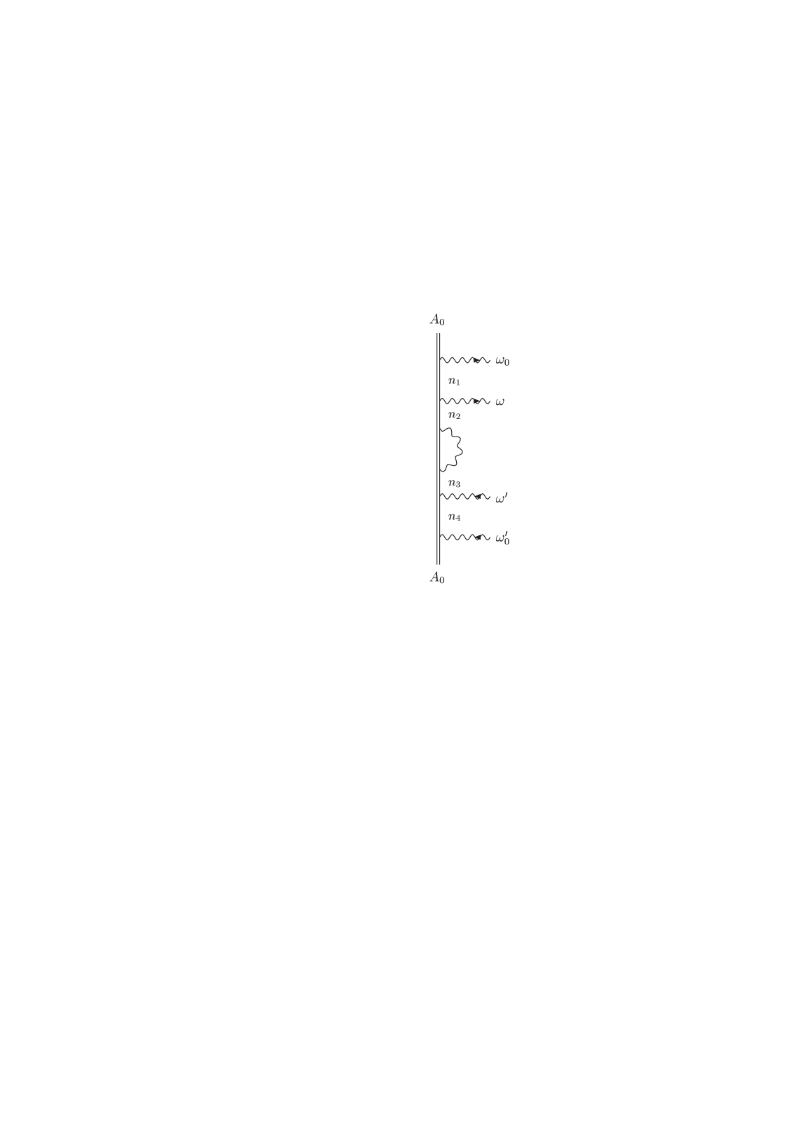
Figure 6: Feynman graph corresponding to the electron self-energy insertion in the central electron propagator in Fig. 5.

We start with the graph depicted in Fig. 6. Having performed the integrations over time and frequency we find

$$U^{(6)}_{\rm{sc}}=\sum_{n_{1}}\frac{(U^{*}_{\omega_{0}})_{A_{0}n_{1}}}{E_{n_{1}}-E_{A_{0}}-\omega_{0}}\sum_{n_{2}n_{3}}\frac{(U^{*}_{\omega})_{n_{1}n_{2}}(\hat{\Sigma}(E_{A_{0}}+\omega_{0}+\omega))_{n_{2}n_{3}}}{(E_{n_{2}}-E_{A_{0}}-\omega_{0}-\omega)(E_{n_{3}}-E_{A_{0}}-\omega_{0}-\omega)}\\ \times\sum_{n_{4}}\frac{(U_{\omega^{\prime}})_{n_{3}n_{4}}(U_{\omega_{0}^{\prime}})_{n_{4}A_{0}}}{E_{n_{4}}-E_{A_{0}}-\omega_{0}-\omega+\omega^{\prime}}\,.$$ (44)

In the resonant case $(n_{1}=A,n_{2}=n_{3}=E_{A^{\prime}},n_{4}=A)$ the equations above yields

$$U^{(6)\rm{res}}_{\rm{sc}} = \frac{(U^{*}_{\omega_{0}})_{A_{0}A}(U^{*}_{\omega})_{AA^{\prime}}}{(E_{A}-E_{A_{0}}-\omega_{0})(E_{A^{\prime}}-E_{A_{0}}-\omega_{0}-\omega)}$$ (45)

$$\times\frac{(\hat{\Sigma}(E_{A_{0}}+\omega_{0}+\omega))_{AA^{\prime}}}{E_{A^{\prime}}-E_{A_{0}}-\omega_{0}-\omega}\,\frac{(U_{\omega^{\prime}})_{A^{\prime}A}(U_{\omega_{0}^{\prime}})_{AA_{0}}}{E_{A}-E_{A_{0}}-\omega_{0}^{\prime}}\,,$$

where the condition (38) has been employed in the last denominator. The resummation of the SE and VP insertions to all orders in perturbation theory leads to the following expression for the emission amplitude

$$U_{\rm{em}}=\frac{(U^{*}_{\omega_{0}})_{A_{0}A}(U^{*}_{\omega})_{AA^{\prime}}}{(E_{A}-E_{A_{0}}-\omega_{0})(\tilde{E}_{A^{\prime}}(\omega+\omega_{0})-E_{A_{0}}-\omega_{0}-\omega)}\,,$$ (46)

where

$$\tilde{E}_{A^{\prime}}(\omega+\omega_{0})=E_{A^{\prime}}+(\hat{\Sigma}(E_{A_{0}}+\omega_{0}+\omega))_{A^{\prime}A^{\prime}}+(V_{U})_{A^{\prime}A^{\prime}}\,.$$ (47)

This result is similar to Eq. (20) which has been derived for the one-photon resonance case. We can also repeat a similar derivation as for the result Eq. (34). For this purpose we should take $n_{1}=A,n_{2}\neq A^{\prime},n_{3}=A^{\prime},n_{4}=A$ in Fig. 6. Accordingly, we find for the emission amplitude

$$U_{\rm{em}}=\frac{(U^{*}_{\omega_{0}})_{A_{0}A}(U^{*}_{\omega})_{A\tilde{A}^{\prime}}}{(E_{A}-E_{A_{0}}-\omega_{0})(\tilde{E}_{A^{\prime}}(\omega+\omega_{0})-E_{A_{0}}-\omega_{0}-\omega)}\,,$$ (48)

where $(U^{*}_{\omega})_{A\tilde{A}^{\prime}}$ is defined by Eq. (36). Eq. (48), as well as Eq. (34) describes the radiative correction to the emission amplitude that improves the wave function of the initial state $A^{\prime}$.

9 Radiative insertions in the upper electron propagator

In this section we turn to the radiative insertions into the upper electron propagator of Fig. 5. To give an example the lowest-order SE insertion is depicted in Fig. 7. Performing again integrations over time and frequency in the corresponding S-matrix element yields

$$U^{(6)}_{\rm{sc}} = \sum_{n_{1}n_{2}}\frac{(U^{*}_{\omega_{0}})_{A_{0}n_{1}}(\hat{\Sigma}(E_{A_{0}}+\omega))_{n_{1}n_{2}}}{(E_{n_{1}}-E_{A_{0}}-\omega_{0})(E_{n_{2}}-E_{A_{0}}-\omega_{0})}$$ (49)

$$\times\sum_{n_{3}}\frac{(U^{*}_{\omega})_{n_{2}n_{3}}}{(E_{n_{3}}-E_{A_{0}}-\omega_{0}-\omega)}\sum_{n_{4}}\frac{(U_{\omega^{\prime}})_{n_{3}n_{4}}(U_{\omega_{0}^{\prime}})_{n_{4}A_{0}}}{(E_{n_{4}}-E_{A_{0}}-\omega_{0}-\omega+\omega^{\prime})}\,.$$

The resonant case is determinated by the conditions: $n_{1}=A,n_{2}=A,n_{3}=A^{\prime},n_{4}=A$, i.e.

$$U^{(6)\rm{res}}_{\rm{sc}} = \frac{(U^{*}_{\omega_{0}})_{A_{0}A}}{E_{A}-E_{A_{0}}-\omega_{0}}\,\frac{(\hat{\Sigma}(E_{A_{0}}+\omega_{0}))_{AA}}{E_{A}-E_{A_{0}}-\omega_{0}}$$

$$\times\frac{(U^{*}_{\omega})_{AA^{\prime}}}{E_{A^{\prime}}-E_{A_{0}}-\omega_{0}-\omega}\,\frac{(U_{\omega^{\prime}})_{A^{\prime}A}(U_{\omega_{0}^{\prime}})_{AA_{0}}}{E_{A}-E_{A_{0}}-\omega_{0}^{\prime}}\,.$$ (50)

We can assume, that all the resonant radiative insertions into the central electron propagator in Fig. 5 are already taken into account. Repeating the radiative insertions in the upper electron line in resonance approximation and summing up the resulting geometrical progression finally yields

$$U_{\rm{em}}=\frac{(U^{*}_{\omega_{0}})_{A_{0}A}(U^{*}_{\omega})_{AA^{\prime}}}{(\tilde{E}_{A}(\omega_{0})-E_{A_{0}}-\omega)(\tilde{E}_{A^{\prime}}(\omega_{0}+\omega)-E_{A_{0}}-\omega_{0}-\omega)}$$ (51)

together with

$$\tilde{E}_{A}(\omega_{0})=E_{A}+(\hat{\Sigma}(E_{A_{0}}+\omega_{0}))_{AA}+(V_{U})_{AA}\,.$$ (52)

Eq. (51) represents the expression for the double-photon amplitude where both energies $E_{A}$ and $E_{A^{\prime}}$ are improved due to radiative corrections.

10 Line profile for the photon emission with energy corrections to the final state

For this purpose it is sufficient to keep only the leading terms in the Taylor expansion of the denominators in Eq. (51):

$$\tilde{E}_{A}(\omega_{0})=E_{A}+(\hat{\Sigma_{A}}(E_{A}))_{AA}+(V_{U})_{AA}=E_{A}+L_{A}-\frac{i}{2}\Gamma_{A}\,,$$ (53)

$$\tilde{E}_{A^{\prime}}(\omega_{0}+\omega)=E_{A^{\prime}}+(\hat{\Sigma_{A^{\prime}}}(E_{A^{\prime}}))_{A^{\prime}A^{\prime}}+(V_{U})_{A^{\prime}A^{\prime}}=E_{A^{\prime}}+L_{A^{\prime}}-\frac{i}{2}\Gamma_{A^{\prime}}\,.$$ (54)

Integrating over both photon directions and summing over the polarizations (see section 4) an expression for the transition probability [41] of double-photon emission is obtained

$$dW_{A^{\prime}\rightarrow A\rightarrow A_{0}} = \frac{1}{(2\pi)^{2}}\frac{\Gamma_{A_{0}A}}{|E_{A}+L_{A}-E_{A_{0}}-\omega_{0}-\frac{i}{2}\Gamma_{A}|^{2}}$$ (55)

$$\times\frac{\Gamma_{AA^{\prime}}\,d\omega d\omega_{0}}{|E_{A^{\prime}}+L_{A^{\prime}}-E_{A_{0}}-\omega_{0}-\omega-\frac{i}{2}\Gamma_{A^{\prime}}|^{2}}\,,$$

where $\Gamma_{A_{0}A},\Gamma_{AA^{\prime}}$ denote the partial widths as defined in section 4. In a next step we integrate over $\omega_{0}$ in the complex plane. The integration can be extended along the real axis $-\infty<\omega_{0}<\infty$ since only the residues at the poles are contributing. We choose the contour in the upper half-plane. The poles are located at

$$\omega^{(1)}_{0} =\omega_{AA_{0}}+L_{A}+\frac{i}{2}\Gamma_{A}\,,$$ (56)

$$\omega^{(2)}_{0} =\omega_{A^{\prime}A_{0}}+L_{A^{\prime}}-\omega+\frac{i}{2}\Gamma_{A^{\prime}}$$ (57)

where $\omega_{AA_{0}}=E_{A}-E_{A_{0}}$ and $\omega_{A^{\prime}A_{0}}=E_{A^{\prime}}-E_{A_{0}}$, respectively. As the result of the integration a new expression for transition probability $dW_{AA^{\prime}}$ is derived, where the Lamb shift and the width of the state $A$ are taken into account

$$dW_{AA^{\prime}} = {\frac{1}{2\pi}}\Gamma_{A_{0}A}\Gamma_{AA^{\prime}}$$ (58)

$$\times\left\{\frac{1}{\Gamma_{A}}\frac{1}{|\omega_{A^{\prime}A_{0}}+L_{A^{\prime}}-\omega_{AA_{0}}-L_{A}-\frac{i}{2}(\Gamma_{A^{\prime}}+\Gamma_{A})-\omega|^{2}}\right.$$

$$\left.+\frac{1}{\Gamma_{A^{\prime}}}\frac{1}{|\omega_{AA_{0}}+L_{A}-\omega_{A^{\prime}A_{0}}-L_{A^{\prime}}-\frac{i}{2}(\Gamma_{A^{\prime}}+\Gamma_{A})+\omega|^{2}}\right\}d\omega\,.$$

After simple algebraic transformations Eq. (58) can be cast into the form

$$dW_{AA^{\prime}}=\frac{1}{2\pi}\frac{\Gamma_{A_{0}A}\Gamma_{AA^{\prime}}}{\Gamma_{A}\Gamma_{A^{\prime}}}\frac{(\Gamma_{A}+\Gamma_{A^{\prime}})\,d\omega}{(\tilde{\omega}_{A^{\prime}A}-\omega)^{2}+\frac{1}{4}(\Gamma_{A^{\prime}}+\Gamma_{A})^{2}}$$ (59)

where $\tilde{\omega}_{A^{\prime}A}=E_{A^{\prime}}+L_{A^{\prime}}-E_{A}-L_{A}$. The latter reveals how the Lamb shift $L_{A}$ of the final state $A$ enters the Lorentz denominator in the expression for the emission probability.

For simplicity, we may assume that $\Gamma_{A_{0}A}=\Gamma_{A}$ and $\Gamma_{AA^{\prime}}=\Gamma_{A^{\prime}}$. This implies that both states $A^{\prime}$ and $A$ have only one decay channel: $A^{\prime}\rightarrow A$ and $A\rightarrow A_{0}$. Finally, we arrive at

$$dW_{AA^{\prime}}=\frac{1}{2\pi}\frac{(\Gamma_{A}+\Gamma_{A^{\prime}})\,d\omega}{(\tilde{\omega}_{A^{\prime}A}-\omega)^{2}+\frac{1}{4}(\Gamma_{A^{\prime}}+\Gamma_{A})^{2}}\,.$$ (60)

This formula does not contain any dependence on the state $A_{0}$. This state enters only indirectly through the definition of $\Gamma_{A}$. If $A$ denotes the ground state, we can set $\Gamma_{A}=0$ in Eq. (60) which yields

$$dW_{AA^{\prime}}=\frac{1}{2\pi}\frac{\Gamma_{A^{\prime}}d\omega}{(\tilde{\omega}_{A^{\prime}A}-\omega)^{2}+\frac{1}{4}\Gamma_{A^{\prime}}^{2}}\,.$$ (61)

The expression above deviates from Eq. (26) only by the presence of the Lamb shift $L_{A}$ in the denominator. The introduction of the state $A_{0}$ acts as a regularization and $\Gamma_{A}$ plays the role of the regularization parameter. In case of the ground state $A$ this parameter is removed by setting it equal to zero at the end of the derivation.

11 Radiative corrections to the emission amplitude (final state)

Now we are in the position to determine the final-state radiative correction to the emission amplitude, i.e. to correct the final-state wave function. For this purpose we return to Fig. 7 and consider the case: $n_{1}=A,n_{2}\neq A,n_{3}=A^{\prime},n_{4}=A$. We assume that the resummation of all radiative insertions in resonance approximation in Fig. 7 is already performed. Instead of Eq. (51) we can write

$$U_{\rm{em}}=\frac{(U^{*}_{\omega_{0}})_{A_{0}A}(U^{*}_{\omega})_{\tilde{A}A^{\prime}}}{(\tilde{E}_{A}(\omega_{0})-E_{A_{0}}-\omega_{0})(\tilde{E}_{A^{\prime}}(\omega_{0}+\omega)-E_{A_{0}}-\omega_{0}-\omega)}\,,$$ (62)

where

$$(U^{*}_{\omega})_{\tilde{A}A^{\prime}}=\sum_{n_{2}\neq A}\frac{\left[(\hat{\Sigma}(E_{A}))_{An_{2}}+(V_{U})_{An_{2}}\right](U^{*}_{\omega})_{n_{2}A^{\prime}}}{E_{n_{2}}-E_{A}}\,.$$ (63)

Comparing Eq. (63) with Eqs. (34) and (36) one can see that it represents the corrections to the final-state wave function in the expression for the emission amplitude.

Collecting now all the various corrections to the amplitudes and to energy denominators given by Eqs. (36), (63), (20) and (52), respectively, we can finally write the generic equation (61) into the form (for the ground state $A$):

$$dW_{AA^{\prime}}=\frac{1}{2\pi}\frac{\Gamma_{\tilde{A}\tilde{A}^{\prime}}d\omega}{(\tilde{\omega}_{A^{\prime}A}-\omega)^{2}+\frac{1}{4}\Gamma^{2}_{A^{\prime}}}\,.$$ (64)

For convenience we reintroduced the notation $\Gamma_{A^{\prime}}=\Gamma_{AA^{\prime}}$ and denoted by $\Gamma_{\tilde{A}\tilde{A}^{\prime}}$ the expression for the width $\Gamma_{A^{\prime}}$ (i.e. for the transition rate $A^{\prime}\rightarrow A$) where both wave functions of the initial $(A^{\prime})$ and final $(A)$ states are corrected according to the formulas (36) and (63). These corrections to the width are additive, so that

$$\Gamma_{\tilde{A}\tilde{A}^{\prime}}=\Gamma_{AA^{\prime}}+\Gamma_{\tilde{A}A^{\prime}}+\Gamma_{A\tilde{A}^{\prime}}$$ (65)

where $\Gamma_{\tilde{A}A^{\prime}}$ and $\Gamma_{A\tilde{A}^{\prime}}$ denote the corrections to $\Gamma_{AA^{\prime}}$ which contain the improved amplitudes (63) and (36).

In principle, the width $\Gamma_{A^{\prime}}$ in the denominator of Eq. (64) also should be replaced by $\Gamma_{\tilde{A}\tilde{A}^{\prime}}$. This means, that a rigorous evaluation of the radiative corrections to the transition probability should include the second-order radiative corrections in the denominator of Eq. (64). The imaginary parts of these second-order corrections would determine exactly the value of $\Gamma_{\tilde{A}\tilde{A}^{\prime}}$ [3].

12 Vertex correction

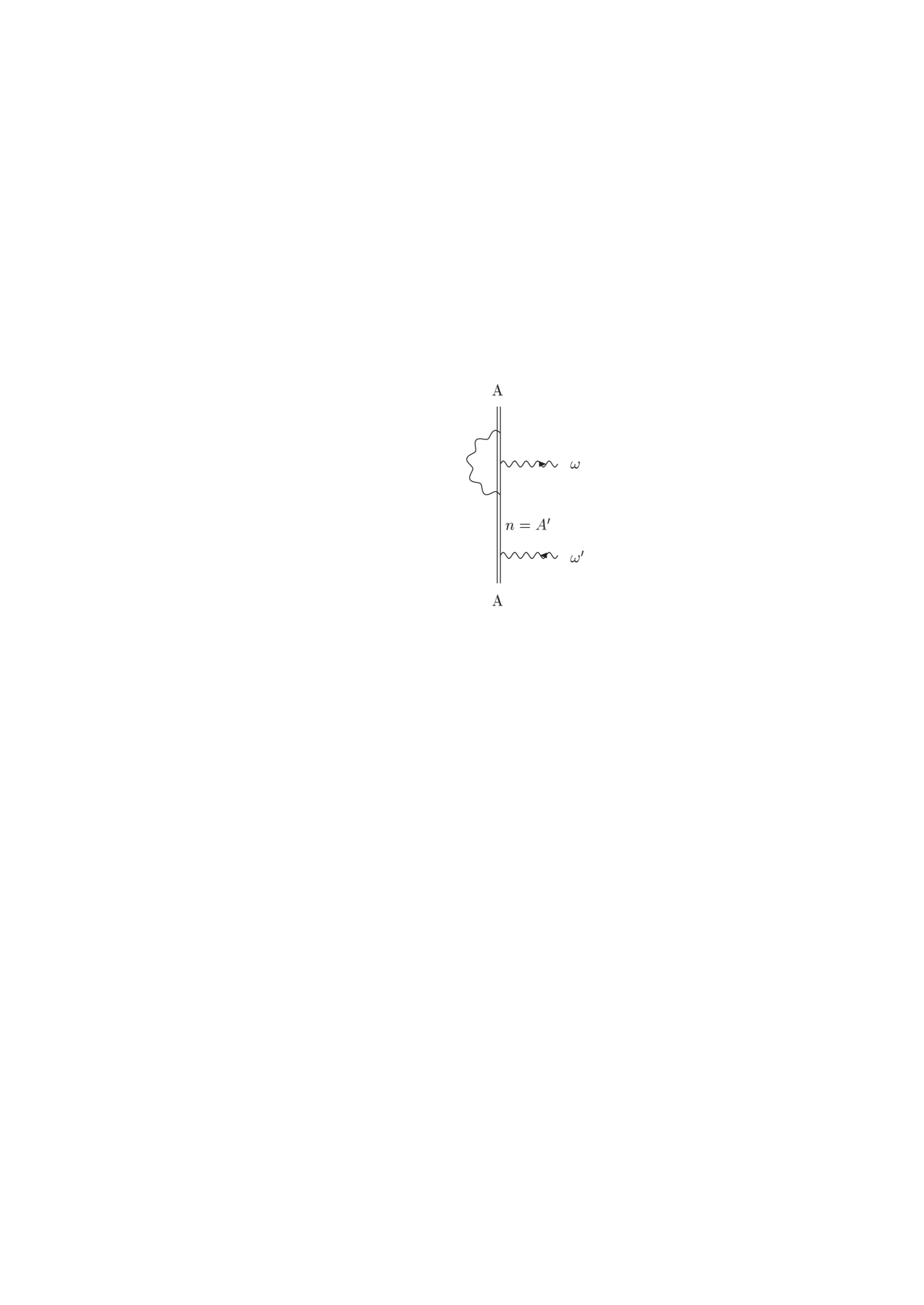
Figure 8: The self-energy vertex correction to the transition amplitude $A^{\prime}\rightarrow A$ in the resonance approximation.

A third type of QED corrections to the emission amplitude, which we have to consider are vertex corrections. For the evaluation of these corrections we can return at first to the one-photon resonance picture (Eq. (18)). The SE vertex correction to the emission amplitude corresponds to the Feynman graph shown in Fig 8. In the resonance approximation this correction reads

$$U^{V}_{\rm{em}}=\frac{(\Lambda^{(1)}_{\mu}A^{\mu*}_{\omega})_{AA^{\prime}}}{\tilde{E}_{A^{\prime}}-E_{A}-\omega}\,,$$ (66)

where $\Lambda^{(1)}_{\mu}$ is the SE vertex that is defined directly by the upper part of the diagram in Fig. 8. The renormalization of $\Lambda^{(1)}_{\mu}$ may be performed in momentum space [40]

$$\Lambda^{(1)\rm{ren}}_{\mu}(\not p^{\prime},\not p)=\Lambda^{(1)}_{\mu}(\not p^{\prime},\not p)-\gamma_{\mu}\Lambda^{(1)}\,,$$ (67)

where

$$\gamma_{\mu}\Lambda^{(1)}=-4\pi ie^{2}\int\frac{d^{4}k}{(2\pi)^{4}}\gamma_{\nu}\frac{\not k}{k^{2}}\gamma_{\mu}\frac{\not k}{k^{2}}\gamma^{\nu}\frac{1}{k^{2}}\,.$$ (68)

In Feynman gauge the counterterm $\gamma_{\mu}\Lambda^{(1)}$ is ultraviolet and infrared divergent. This divergency cancels, if we take into account another contribution to the SE vertex that follows from the graph Fig. 2 and which has not yet been considered. Without changing the results of Section 3 we can take the first term of the geometric progression with SE corrections and multiply the expression without radiative corrections (i.e., the right-hand side of Eq. (18)) by this term:

$$U^{o}_{\rm{em}}+U^{d}_{\rm{em}}=-\frac{(\gamma_{\mu}A^{\omega*}_{\mu})_{AA^{\prime}}}{\tilde{E}_{A^{\prime}}-E_{A}-\omega}\,\frac{(\hat{\Sigma}(E_{A}+\omega))_{A^{\prime}A^{\prime}}}{E_{A^{\prime}}-E_{A}-\omega}\,.$$ (69)

Here we employ the notation $U^{o}_{\rm{em}}$ for the emission amplitude Eq. (18) without radiative corrections and $U^{d}_{\rm{em}}$ stands for ”derivative” correction that will follow from Eq. (69).

Using the Taylor expansion (19) for $\Sigma(E_{A}+\omega)$ and substituting the resonant value (29) for the frequency $\omega=\omega^{(1)}_{\rm{res}}=E_{A^{\prime}}+\Sigma_{A^{\prime}}-E_{A}$ into the energy denominator in Eq. (69), we obtain

$$U^{o}_{\rm em}+U^{d}_{\rm{em}}=-\frac{(\gamma_{\mu}A^{\omega*}_{\mu})_{AA^{\prime}}}{\tilde{E}_{A^{\prime}}-E_{A}-\omega}\left[1+(\hat{\Sigma}^{\prime}(E_{A^{\prime}}))_{A^{\prime}A^{\prime}}\right]\,,$$ (70)

respectively

$$U^{o}_{\rm em}+U^{d}_{\rm em}+U^{V}_{\rm em} = -\frac{(U^{*}_{\omega})_{AA^{\prime}}}{\tilde{E}_{A^{\prime}}-E_{A}-\omega}$$ (71)

$$+\frac{1}{\tilde{E}_{A^{\prime}}-E_{A}-\omega}\left[(\Lambda^{(1)}_{\mu}A^{\mu*}_{\omega})_{AA^{\prime}}+\Sigma^{\prime}_{A^{\prime}}(\gamma_{\mu}A^{\mu*}_{\omega})_{AA^{\prime}}\right]\,.$$

The renormalized expression for $\hat{\Sigma}^{\prime}$ is given by [40]

$${\hat{\Sigma^{\prime}}}^{\rm{ren}}(\not p)={\hat{\Sigma^{\prime}}}(\not p)-\Sigma^{\prime}\,,$$ (72)

where

$$\left.\gamma_{\mu}\Sigma^{\prime}\equiv\frac{\partial}{\partial p_{\mu}}\hat{\Sigma}(\not p)\right|_{\not p=m}$$ (73)

and $\hat{\Sigma}(\not{p})$ denotes the lowest-order electron self-energy operator in momentum space. The counterterm $\Sigma^{\prime}$ contains ultraviolet and infrared divergencies. Due to the Ward identity

$$\Lambda^{(1)}=-\Sigma^{\prime}$$ (74)

all the divergencies in Eq. (71) cancel. The total renormalized expression Eq. (71) seems to be asymmetric with respect to $A$ and $A^{\prime}$. A symmetric result can be obtained from the two-photon resonance scattering.

Consider now Eq. (51). Repeating similar derivations as have been performed above for Eq. (18), we obtain

$$U^{o}_{\rm{em}}+U^{d}_{\rm{em}}=\frac{1}{2}\frac{(U^{*}_{\omega_{0}})_{A_{0}A}(U^{*}_{\omega})_{AA^{\prime}}}{(\tilde{E}_{A}(\omega_{0})-E_{A_{0}}-\omega)(\tilde{E}_{A^{\prime}}(\omega_{0}+\omega)-E_{A_{0}}-\omega_{0}-\omega)}\\ \times\left\{\left(-\frac{\Sigma_{A^{\prime}}}{E_{A^{\prime}}-E_{A_{0}}-\omega^{(0)}_{0\rm res}-\omega^{(1)}_{\rm res}+{\Sigma^{\prime}}^{(\rm ren)}_{A^{\prime}}}\right)\right.\\ +\left.\left(-\frac{\Sigma_{A^{\prime}}}{E_{A}-E_{A_{0}}-\omega^{(1)}_{0\rm res}+{\Sigma^{\prime}}^{(\rm ren)}_{A}}\right)\right\}\,,$$ (75)

together with the lowest-order resonance energies

$$\omega^{(0)}_{0\rm res} = E_{A}-E_{A_{0}}\,,$$ (76)

$$\omega^{(1)}_{0\rm res} = E_{A}-E_{A_{0}}+\Sigma_{A}\,,$$ (77)

$$\omega^{(1)}_{\rm{res}} = E_{A^{\prime}}-E_{A}+\Sigma_{A^{\prime}}\,.$$ (78)

We omit here VP contributions in the denominators of Eq. (75). The values $\Sigma_{A}\equiv(\hat{\Sigma}(E_{A}))_{AA}$ and $\Sigma_{A^{\prime}}\equiv(\hat{\Sigma}(E_{A^{\prime}}))_{A^{\prime}A^{\prime}}$ are considered as being renormalized $\Sigma_{A}=\Sigma^{\rm(ren)}_{A}$, $\Sigma_{A^{\prime}}=\Sigma^{\rm{(ren)}}_{A^{\prime}}$. Substitution of Eqs. (76), (77), (78) into Eq. (75) yields a symmetrized expression for the sum:

$$U^{o}_{\rm em}+U^{d}_{\rm em}=\frac{(U^{*}_{\omega_{0}})_{A_{0}A}(U^{*}_{\omega})_{AA^{\prime}}}{(\tilde{E}_{A}(\omega_{0})-E_{A_{0}}-\omega)(\tilde{E}_{A^{\prime}}(\omega_{0}+\omega)-E_{A_{0}}-\omega_{0}-\omega)}\\ \times\left(1+\frac{1}{2}\left[\Sigma^{{}^{\prime}\rm{(ren)}}_{A^{\prime}}+{\Sigma^{\prime}}^{\rm{(ren)}}_{A}\right]\right)\,.$$ (79)

The cancellation of the divergencies with those in $U^{V}_{\rm{em}}$ still takes place.

Now the expression (65) requires to correct the width by replacing $\Gamma_{\tilde{A}\tilde{A}^{\prime}}$ by $\tilde{\Gamma}_{\tilde{A}\tilde{A}^{\prime}}$ where

$$\tilde{\Gamma}_{\tilde{A}\tilde{A}^{\prime}}=\tilde{\Gamma}_{AA^{\prime}}+{\Gamma}_{\tilde{A}A^{\prime}}+{\Gamma}_{A\tilde{A}^{\prime}}\,.$$ (80)

The width $\tilde{\Gamma}_{AA^{\prime}}$ results from Eq. (26) by replacing the amplitudes $U_{\rm{em}}$ by the modified expressions Eq. (71) and (79), respectively.

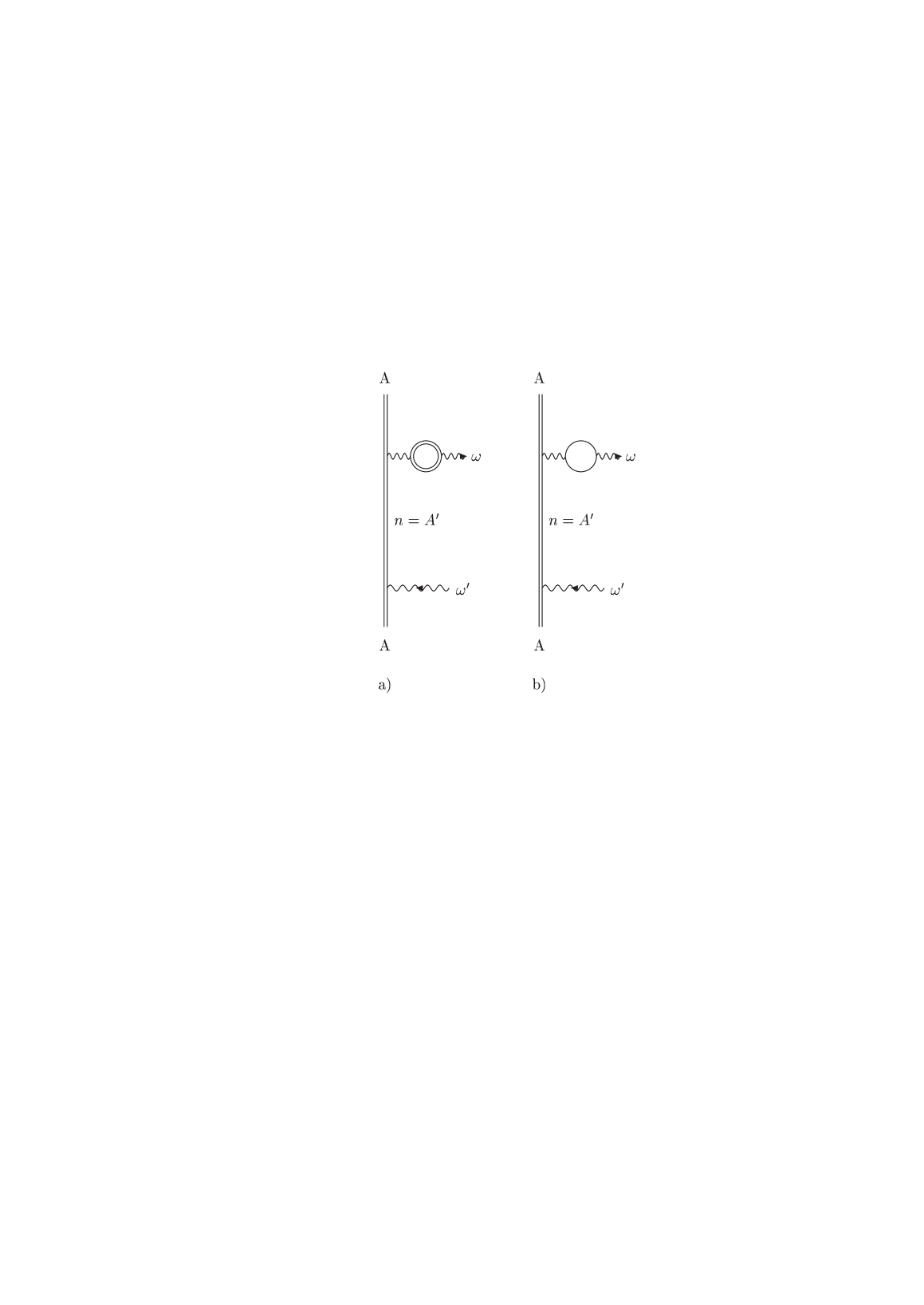
Figure 9: The vacuum polarization vertex correction to the transition amplitude $A^{\prime}\rightarrow A$ in the resonance approximation: a) exact expression, b) Uehling approximation.

What further remains is to include the contribution of the VP vertex as depicted in Fig. 9. In Uehling approximation the renormalization of the corresponding correction is straightforward. One has to replace the expression for the electron loop in Fig. 9 b), i.e. the photon self energy $\Pi(x_{1}x_{2})$ by the known renormalized expression $\Pi_{R}$ [41].

13 Weak interaction mixed amplitude

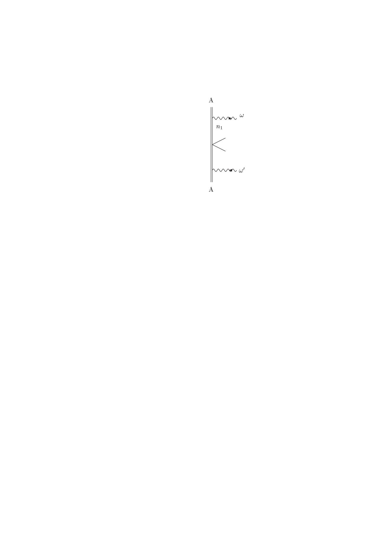
Figure 10: Feynman graph that describes the elastic photon scattering on an atomic electron in the presence of weak interaction. The effective potential of weak interaction between the electron and the nucleus is denoted by a ”sea-gull”.

To begin the investigation of additional corrections to the amplitude due to weak interaction we return to the generic one-photon scattering Feynman diagram Fig. 1 by adding at first the effective weak-interaction potential in the electron propagator (see Fig. 10). We can specify the corresponding scattering amplitude as

$$U_{\rm{sc}}=\sum_{n_{1}}\frac{(U^{*}_{\omega})_{An_{1}}}{E_{n_{1}}-E_{A}-\omega}\sum_{n_{2}}\frac{(\gamma_{0}V_{\rm{PNC}})_{n_{1}n_{2}}(U_{\omega^{\prime}})_{n_{2}A}}{E_{n_{2}}-E_{A}-\omega}\,,$$ (81)

together with the effective parity-nonconserving (PNC) potential

$$V_{\rm{PNC}}=-\frac{G_{F}}{2\sqrt{2}}Q_{w}\rho_{N}(r)\gamma_{5}\,.$$ (82)

$Q_{w}$ denotes the ”weak charge” of the nucleus

$$Q_{w}=Z(1-4\sin^{2}\Theta_{w})-N\,,$$ (83)

which relates the numbers of protons $Z$ and neutrons $N$ in the nucleus and the Weinberg angle $\Theta_{w}$ - the free parameter of the electroweak theory. The latter is usually determined via a comparison between theoretical predictions and data from various experiments both in high-energy and atomic physics. The recent adopted value for the Weinberg angle is $\Theta_{w}=0.2312$ [42].

Within the resonance approximation we set $n_{2}=A^{\prime}$ in Eq. (81). Since the operator $V_{\rm{PNC}}$ has no diagonal matrix elements the term $n_{1}=A^{\prime}$ is absent. However, we can choose a level $n_{1}=A^{\prime\prime}$ which gives a dominant contribution to the sum over $n_{1}$. A standard example in atomic physics is: $A=1s,A^{\prime}=2s,A^{\prime\prime}=2p$. Accordingly in the sum over $n_{1}$ the term yielding the small denominator $E_{A^{\prime\prime}}-E_{A^{\prime}}$ (in the resonance approximation) dominates. The emission amplitude reads

$$U_{\rm{em}}=\frac{(U^{*}_{\omega})_{AA^{\prime\prime}}}{E_{A^{\prime\prime}}-E_{A}-\omega}\,\frac{(\gamma_{0}V_{\rm PNC})_{A^{\prime\prime}A^{\prime}}}{E_{A^{\prime}}-E_{A}-\omega}\,.$$ (84)

Introducing the resonance frequency in the first denominator we can further write

$$U_{\rm{em}}=\frac{(U^{*}_{\omega})_{AA^{\prime\prime}}}{E_{A^{\prime\prime}}-E_{A^{\prime}}}\,\frac{(\gamma_{0}V_{\rm{PNC}})_{A^{\prime\prime}A^{\prime}}}{E_{A^{\prime}}-E_{A}-\omega}\,.$$ (85)

In particular for states $A^{\prime}=2s,A^{\prime\prime}=2p$ in the approximation of noninteracting electrons $E_{A^{\prime\prime}}=E_{A^{\prime}}$. This implies that in the first denominator in Eq. (85) one has to account for the Lamb shift $\Delta E_{L}$. In the next section we will show how it arises and how to use the form (84) for $U_{\rm{em}}$ for this purpose.

14 Radiative corrections to the weak interaction mixed amplitude

The first step consist in the evaluation of the SE insertions in the upper electron propagator in the diagram of Fig. 10 within the resonance approximation (see Fig. 11 for the first term of this sequence).

The scattering amplitude, corresponding to the diagram of Fig. 11 is given by

$$U_{\rm{sc}}=\sum_{n_{1}}\frac{(U^{*}_{\omega})_{An_{1}}}{E_{n_{1}}-E_{A}-\omega}\sum_{n_{2}n_{3}}\frac{(\hat{\Sigma}(E_{A}+\omega))_{n_{1}n_{2}}(\gamma_{0}V_{\rm{PNC}})_{n_{2}n_{3}}(U_{\omega^{\prime}})_{n_{3}A}}{(E_{n_{2}}-E_{A}-\omega)(E_{n_{3}}-E_{A}-\omega)}\,.$$ (86)

The resonant state is $n_{3}=E_{A^{\prime}}$. The states yielding dominant contributions are $n_{1}=n_{2}=E_{A^{\prime\prime}}$. Keeping only these terms in the summations we obtain

$$U_{\rm{em}}=\frac{(U^{*}_{\omega})_{AA^{\prime\prime}}}{E_{A^{\prime\prime}}-E_{A}-\omega}\,\frac{(\hat{\Sigma}(E_{A}+\omega))_{A^{\prime\prime}A^{\prime\prime}}}{(E_{A^{\prime\prime}}-E_{A}-\omega)}\,\frac{(\gamma_{0}V_{\rm{PNC}})_{A^{\prime\prime}A^{\prime}}}{E_{A^{\prime}}-E_{A}-\omega}\,.$$ (87)

In resonance approximation we can set $E_{A}+\omega=E_{A^{\prime}}$ in the matrix element $(\hat{\Sigma}(E_{A}+\omega))_{A^{\prime\prime}A^{\prime\prime}}$ and, furthermore, $E_{A^{\prime}}=E_{A^{\prime\prime}}$ due to the almost degeneracy of the levels $A^{\prime}$ and $A^{\prime\prime}$. Then the resummation of the SE insertions yields

$$U_{\rm{em}}=\frac{(U^{*}_{\omega})_{AA^{\prime\prime}}}{\tilde{E}_{A^{\prime\prime}}-E_{A}-\omega}\,\frac{(\gamma_{0}V_{\rm{PNC}})_{A^{\prime\prime}A^{\prime}}}{E_{A^{\prime}}-E_{A}-\omega}\,.$$ (88)

If $n_{1}=A^{\prime\prime}$ but $n_{2}\neq A^{\prime\prime}$, we obtain the correction to the PNC matrix element $(V_{\rm{PNC}})_{A^{\prime\prime}A^{\prime}}$ (assuming that all insertions in the resonant approximation are already performed)

$$U_{\rm{em}} =\frac{(U^{*}_{\omega})_{AA^{\prime\prime}}}{\tilde{E}_{A^{\prime\prime}}-E_{A}-\omega}\,\frac{(\gamma_{0}V_{\rm{PNC}})_{\tilde{A}^{\prime\prime}A^{\prime}}}{E_{A^{\prime}}-E_{A}-\omega}\,,$$ (89)

$$(\gamma_{0}V_{\rm{PNC}})_{\tilde{A}^{\prime\prime}A^{\prime}} =\sum_{n_{2}\neq A^{\prime\prime}}\frac{(\hat{\Sigma}(E_{A^{\prime\prime}}))_{A^{\prime\prime}n_{2}}(\gamma_{0}V_{\rm{PNC}})_{n_{2}A^{\prime}}}{E_{n_{2}}-E_{A^{\prime\prime}}}\,,$$ (90)

together with $E_{A^{\prime}}=E_{A^{\prime\prime}}$ in the denominator. This represents the correction to the wave function $A^{\prime\prime}$ in the PNC matrix element.

In order to account for vacuum-polarization insertions we simply have to replace Eq. (90) by

$$(\gamma_{0}V_{\rm{PNC}})_{\tilde{A}^{\prime\prime}A^{\prime}}=\sum_{n_{2}\neq A^{\prime\prime}}\frac{\left[(\hat{\Sigma}(E_{A^{\prime\prime}}))_{A^{\prime\prime}n_{2}}+(V_{U})_{A^{\prime\prime}n_{2}}\right](\gamma_{0}V_{\rm{PNC}})_{n_{2}A^{\prime}}}{E_{n_{2}}-E_{A^{\prime\prime}}}\,.$$ (91)

A vacuum-polarization correction of this kind has been calculated numerically in [32].

Now we turn to the evaluation of the SE insertions in the lower electron propagator in Fig. 10 (see Fig. 12). The corresponding scattering amplitude is

$$U_{\rm{sc}}=-\sum_{n_{1}}\frac{(U^{*}_{\omega})_{An_{1}}}{E_{n_{1}}-E_{A}-\omega}\sum_{n_{2}n_{3}}\,\frac{(\gamma_{0}V_{\rm{PNC}})_{n_{1}n_{2}}(\hat{\Sigma}(E_{A}+\omega))_{n_{2}n_{3}}(U_{\omega^{\prime}})_{n_{3}A}}{(E_{n_{2}}-E_{A}-\omega)(E_{n_{3}}-E_{A}-\omega)}\,.$$

In this case the dominant state is $n_{1}=A^{\prime\prime}$ and the resonant states are $n_{2}=n_{3}=A^{\prime}$, respectively. The expression for the emission amplitude can now be expressed as

$$U_{\rm{em}}=-\frac{(U^{*}_{\omega})_{AA^{\prime\prime}}}{E_{A^{\prime\prime}}-E_{A}-\omega}\,\frac{(\gamma_{0}V_{\rm{PNC}})_{A^{\prime\prime}A^{\prime}}}{E_{A^{\prime}}-E_{A}-\omega}\,\frac{(\hat{\Sigma}(E_{A}+\omega))_{A^{\prime}A^{\prime}}}{(E_{A^{\prime}}-E_{A}-\omega)}\,.$$ (93)

After resummation of SE insertions for the resonant state $A^{\prime}$ to all orders, we obtain

$$U_{\rm{em}}=\frac{(U^{*}_{\omega})_{AA^{\prime\prime}}}{\tilde{E}_{A^{\prime\prime}}-E_{A}-\omega}\,\frac{(\gamma_{0}V_{\rm{PNC}})_{A^{\prime\prime}A^{\prime}}}{\tilde{E}_{A^{\prime}}-E_{A}-\omega}=\frac{(U^{*}_{\omega})_{AA^{\prime\prime}}}{\tilde{E}_{A^{\prime\prime}}-\tilde{E}_{A^{\prime}}}\,\frac{(\gamma_{0}V_{\rm{PNC}})_{A^{\prime\prime}A^{\prime}}}{\tilde{E}_{A^{\prime}}-E_{A}-\omega}\,.$$ (94)

Here we have used the resonance condition $\omega=\tilde{E}_{A^{\prime}}-E_{A}$.

Again, the summation of all SE corrections in Fig. 11 is supposed to be already performed. Moreover, we will assume that VP contributions are included in both Fig. 11 and Fig. 12, respectively. Accordingly, we can write

$$U_{\rm{em}}=\frac{(U^{*}_{\omega})_{AA^{\prime\prime}}}{\tilde{E}_{A^{\prime}}-E_{A}-\omega}\,\frac{(\gamma_{0}V_{\rm{PNC}})_{A^{\prime\prime}A^{\prime}}}{\Delta E_{L}}\,,$$ (95)

together with $\Delta E_{L}=L_{A^{\prime\prime}}-L_{A^{\prime}}$. Eq. (95) holds for the degenerated case, when $E_{A^{\prime}}=E_{A^{\prime\prime}}$.

Setting $n_{2}\neq A^{\prime}$ in Fig. 12 we obtain the correction to the PNC matrix element (respectively to the wave function of the state $A^{\prime\prime}$):

$$U_{\rm{em}}=\frac{(U^{*}_{\omega})_{AA^{\prime\prime}}}{\tilde{E}_{A^{\prime}}-E_{A}-\omega}\,\frac{(\gamma_{0}V_{\rm{PNC}})_{A^{\prime\prime}\tilde{A}^{\prime}}}{\Delta E_{L}}\,,$$ (96)

where

$$(\gamma_{0}V_{\rm{PNC}})_{A^{\prime\prime}\tilde{A}^{\prime}}=\sum_{n_{2}\neq A^{\prime}}\frac{(\gamma_{0}V_{\rm{PNC}})_{A^{\prime\prime}n_{2}}\left[(\hat{\Sigma}(E_{A^{\prime\prime}}))_{n_{2}A^{\prime}}+(V_{U})_{n_{2}A^{\prime}}\right]}{E_{n_{2}}-E_{A^{\prime}}}$$ (97)

A similar replacement $E_{A^{\prime\prime}}-E_{A}-\omega\rightarrow\Delta E_{L}$ can be performed in Eq. (89).

Graphs with $V_{\rm{PNC}}$ inserted in the outer electron lines in Fig. 10 are less important since they do not contain dominant terms with small denominators.

15 Electromagnetic vertex correction to the weak interaction mixed amplitude

The weak interaction amplitude with one-loop SE corrections at the PNC vertex is described by the Feynman diagram in Fig. 13. The corresponding expression for this correction, denoted as $U^{\rm{VW}}_{\rm{sc}}$, can be written as

$$U^{\rm{VW}}_{\rm{sc}}=-\sum_{n_{1}n_{2}}\frac{(U^{*}_{\omega})_{An_{1}}(\Lambda^{(1)W}_{\mu}B^{\mu})_{n_{1}n_{2}}(U^{*}_{\omega^{\prime}})_{n_{2}A}}{(E_{n_{1}}-E_{A}-\omega)(E_{n_{2}}-E_{A}-\omega)}\,.$$ (98)

Here $\Lambda^{(1)W}_{\mu}$ is the weak interaction vertex that differs from the pure electromagnetic vertex $\Lambda^{(1)}_{\mu}$ as discussed in section 12 by changing the vector-coupling $\gamma_{\mu}$ that enters in the expression for $\Lambda^{(1)}_{\mu}$ to the pseudo-vector matrix $\gamma_{5}\gamma_{\mu}$.

A weak interaction potential $B_{\mu}$ according to Eq. (82) may be introduced by

$$B_{\mu}=-\delta_{\mu_{0}}\frac{G_{F}}{2\sqrt{2}}Q_{W}\rho_{N}(r)\,.$$ (99)

Evaluating Eq. (99) within the resonance approximation implies $n_{2}=A^{\prime}$ together with $n_{1}=A^{\prime\prime}$ as the dominant state.

Again we assume that the resummation of radiative insertions in both electron propagators in Fig. 10 is already performed:

$$U^{\rm{VW}}_{\rm{em}}=\frac{(U^{*}_{\omega})_{AA^{\prime\prime}}}{\tilde{E}_{A^{\prime}}-E_{A}-\omega}\,\frac{(\Lambda^{(1)W}_{\mu}B^{\mu})_{A^{\prime\prime}A^{\prime}}}{\Delta E_{L}}\,.$$ (100)

The vertex $\Lambda^{(1)W}_{\mu}$ is ultraviolet and infrared divergent. The renormalization scheme can be taken over from the pure electromagnetic vertex:

$$\Lambda^{(1)\rm{W(ren)}}_{\mu} =\Lambda^{(1)W}_{\mu}(\not p^{\prime},\not p)-\gamma_{\mu}\Lambda^{(1)W}\,,$$ (101)

$$\gamma_{\mu}\Lambda^{(1)W} \left.\equiv\Lambda^{(1)W}_{\mu}(\not p^{\prime},\not p)\right|_{\not p^{\prime}=\not p=m}\,.$$ (102)

In view of Eq. (68) we can write

$$\gamma_{\mu}\Lambda^{(1)W}=-4\pi e^{2}\int\frac{d^{4}k}{(2\pi)^{4}}\gamma_{nu}\frac{\not k}{k^{2}}\gamma_{5}\gamma_{\mu}\frac{\not k}{k^{2}}\gamma^{\nu}\frac{1}{k^{2}}=\gamma_{5}\gamma_{\mu}\Lambda^{(1)}\,.$$ (103)

Similarly, the cancellation of the divergency in $U^{\rm{VW}}_{\rm{em}}$ occurs through the derivative corrections. Consider once more diagrams with SE insertions of the type as depicted in Fig. 11. Without changing the results of section 14 we can proceed with the first term of the geometric progression in the same manner as it was done in section 12. This yields

$$U^{0\rm{W}}_{\rm{em}}+U^{dW}_{\rm{em}}=\frac{(U^{*}_{\omega})_{AA^{\prime\prime}}}{\tilde{E}_{A^{\prime}}-E_{A}-\omega}\,\frac{(\gamma_{0}V_{\rm{PNC}})_{A^{\prime\prime}A^{\prime}}}{\Delta E_{L}}\left(1+\Sigma_{A^{\prime}}^{{}^{\prime}(\rm{ren})}\right)\,.$$ (104)

Combining Eq. (104) with Eq. (100) we have

$$U^{0W}_{\rm{em}}+U^{\rm{VW}}_{\rm{em}}+U^{dW}_{\rm{em}}=\frac{(U^{*}_{\omega})_{AA^{\prime\prime}}}{\tilde{E}_{A^{\prime}}-E_{A}-\omega}\frac{1}{\Delta E_{L}}\\ \times\left[(\gamma_{0}V_{\rm{PNC}})_{A^{\prime\prime}A^{\prime}}+(\Lambda^{(1)W(\rm{ren})}_{\mu}B^{\mu})_{A^{\prime\prime}A^{\prime}}+\Sigma_{A^{\prime}}^{{}^{\prime}(\rm ren)}(\gamma_{0}V_{\rm{PNC}})_{A^{\prime\prime}A^{\prime}}\right]\,.$$ (105)

Since $V_{\rm{PNC}}=\gamma_{5}B_{0}$ we find that the divergent part of the second term in the square brackets in Eq. (105) is $-\Lambda^{(1)}(\gamma_{0}V_{\rm{PNC}})_{A^{\prime\prime}A^{\prime}}$, while the divergent part of the third term in square brackets is $-\Sigma^{(1)^{\prime}}(\gamma_{0}V_{\rm{PNC}})_{A^{\prime\prime}A^{\prime}}$. These divergent parts cancel due to the Ward identity. The total expression can be rewritten in symmetric form when performing the same manipulations with the first term of the geometric progression in Fig. 12. As a result, we find

$$U^{w}_{\rm em}=U^{0w}_{\rm{em}}+U^{VW}_{\rm{em}}+U^{dW}_{\rm{em}}=\frac{(U^{*}_{\omega})_{AA^{\prime\prime}}}{{\tilde{E}}_{A^{\prime}}-E_{A}-\omega}\frac{1}{\Delta E_{L}}\\ \times\left[(\gamma_{0}V_{\rm{PNC}})_{{A^{\prime}}^{\prime}A^{\prime}}+(\Lambda^{(1)W({\rm ren})}_{\mu}B^{\mu})_{A^{\prime\prime}A^{\prime}}+\frac{1}{2}(\Sigma_{A^{\prime}}^{{}^{\prime}\rm{(ren)}}+\Sigma_{A^{\prime\prime}}^{{}^{\prime}\rm{(ren)}})\right](\gamma_{0}V_{\rm{PNC}})_{A^{\prime\prime}A^{\prime}}\,.$$ (106)

In principle, there exists also the VP electromagnetic vertex correction depicted in Fig. 14. However, as it was shown in [32], this correction turns out to vanish within Uehling approximation.

Finally, we can represent all pure electromagnetic radiative corrections to the PNC matrix element in the form

$$(\gamma_{0}\tilde{V}_{\rm{PNC}})_{A^{\prime\prime}A^{\prime}}=(\gamma_{0}V_{\rm{PNC}})_{A^{\prime\prime}A^{\prime}}+(\gamma_{0}V_{\rm{PNC}})_{\tilde{A}^{\prime\prime}A^{\prime}}+(\gamma_{0}V_{\rm{PNC}})_{A^{\prime\prime}\tilde{A}^{\prime}}\\ +(\Lambda^{(1)w(\rm ren)}_{\mu}B^{\mu})_{A^{\prime\prime}A^{\prime}}+\frac{1}{2}\left(\Sigma_{A^{\prime}}^{{}^{\prime}(\rm ren)}+\Sigma_{A^{\prime\prime}}^{{}^{\prime}(\rm ren)}\right)(\gamma_{0}V_{PNC})_{A^{\prime\prime}A^{\prime}}\,.$$ (107)

The VP parts of the corrections $(\gamma_{0}V_{\rm{PNC}})_{A^{\prime\prime}\tilde{A}^{\prime}}$ and $(\gamma_{0}V_{\rm{PNC}})_{\tilde{A}^{\prime\prime}A^{\prime}}$ have been calculated earlier in [32].

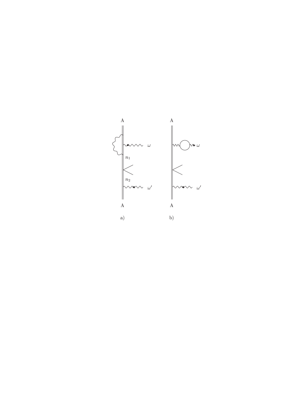
Figure 15: Vertex corrections to the emission matrix element in the weak emission amplitude a) self-energy vertex correction b) vacuum polarization vertex correction in Uehling approximation.

Apart from corrections to the weak interaction matrix element there exist also corrections to the emission matrix element in the weak interaction emission amplitude. They either result by setting $n_{1}\neq A^{\prime\prime}$, but $n_{2}=A^{\prime\prime}$ in Eq. (14) or by inserting radiative corrections into the upper external electron line in the diagram of Fig. 12. In the latter case one may turn over again to the double photon resonance picture described in sections 7-11. The other corrections to the emission matrix element are given by the Feynman graphs in Fig. 15. These corrections can be treated in the same manner as vertex corrections in the case of a pure electromagnetic amplitude (section 12).

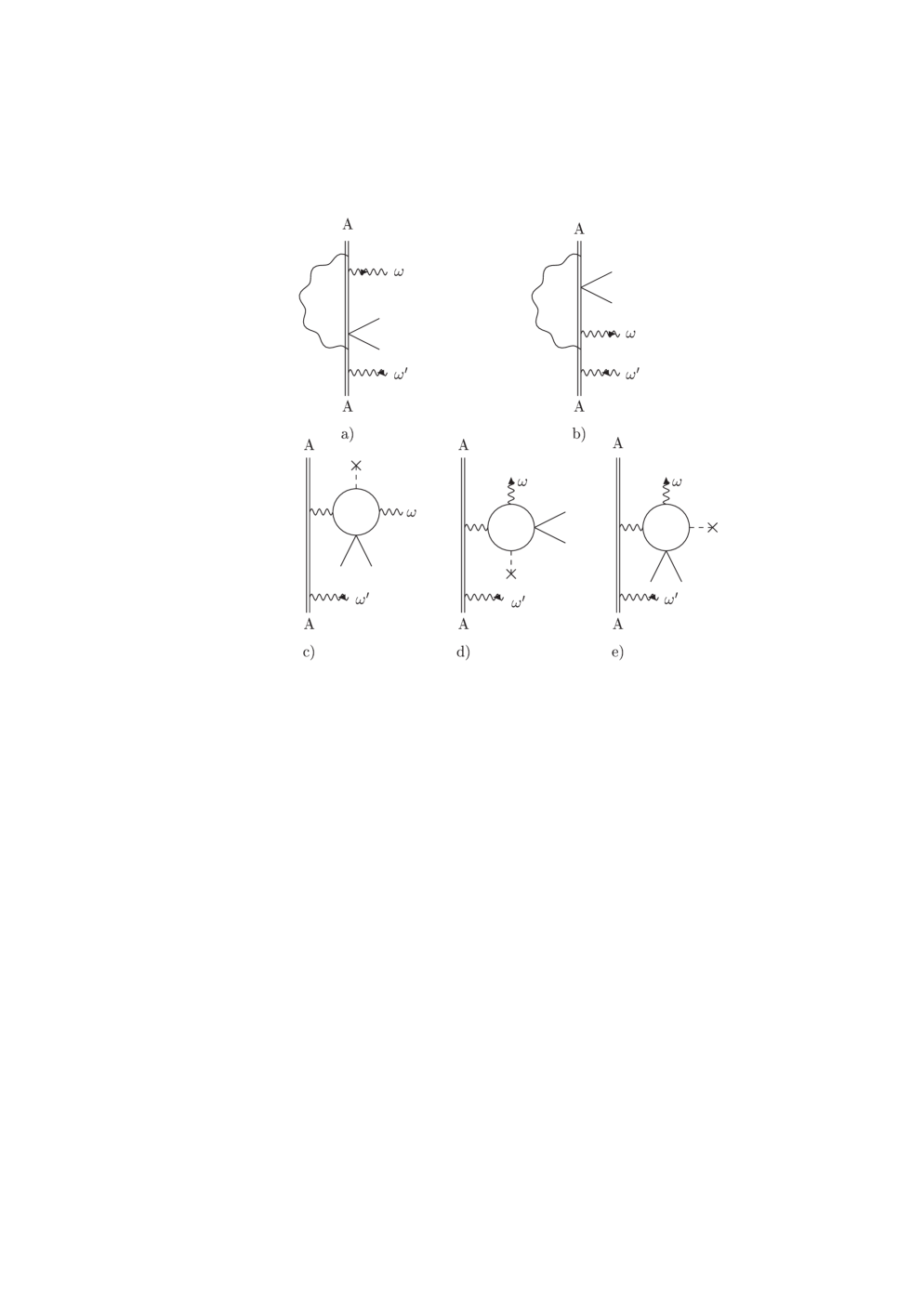
Figure 16: Unseparable radiative corrections to the weak emission amplitude. Figs. 16 a), b) correspond to self-energy corrections, Figs. 16 c)-e) correspond to vacuum polarization corrections in Uehling approximation.

Note, that there exist unseparable radiative effects which cannot be adjusted to the weak interaction matrix element or to the emission matrix element in the weak interaction emission amplitude. These corrections are depicted in Fig. 16. However, they do not generate small energy denominators of the type $(\Delta E_{L})^{-1}$ and thus are neglible compared to the corrections (107). Nevertheless, they have to be taken into account if for some reasons the small denominator is absent.

16 The interelectron interaction insertions in the electron propagators

In this section we begin to investigate the line profiles and transition rates in two-electron ions. The same formalism will be applicable to few-electron ions as well.

For highly-charged ions the lowest-order radiative corrections and the lowest-order interelectron interaction corrections (IIC) are approximately of the same magnitude. While the first ones are of the order $\alpha=e^{2}$ the second ones are of the order $1/Z$ which is the same for $\alpha Z\sim 1$. Since the lowest-order radiative corrections and IIC are additive the radiative effects can be taken over from case of the one-electron ions (sections 2-12). What remains is to include the lowest order IIC, i.e. one-photon exchange corrections.

The first-, second- and partly the third-order IIC to the energy levels have been calculated within the framework of QED during the last decade for two- and three-electron ions [43]- [47], [24]. In particular, the line-profile approach was used for the evaluation of the reducible parts of the two- and three-photon exchange corrections in [24], [48], [23].

However, the interelectron interaction corrections to the transition probabilities have not been studied so thoroughly. In this and the following sections of our paper we present a full QED approach to the evaluation of the IIC based on the line profile theory. We will mainly concentrate on the first-order IIC, although the generalization to higher orders is straightforward.

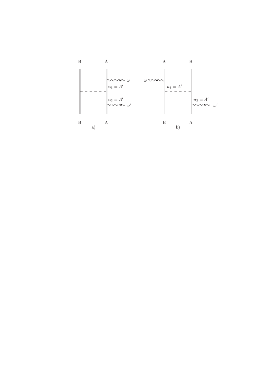
Figure 17: The Feynman graphs that describe the elastic photon scattering on a two-electron ion in resonance approximation with first-order Coulomb interelectron interaction corrections taken into account. Here $A,B$ denote one-electron states in the two-electron ion, $A^{\prime}$ is the resonant state. The dashed line corresponds to the Coulomb photon. The graph Fig. 17a) describes the ”direct” term in the amplitude and the graph Fig. 17b) corresponds to the ”exchange” term. The contributions of the ”exchange” graphs always enter with an additional minus sign which traces back to the antisymmetrization of the two-electron wave function.

Consider the elastic photon scattering on a two-electron ion with the first-order IIC taken into account. We assume that scattering occurs at the electron in the state $A$, while the electron in the state $B$ plays the role of a spectator. This process is depicted in Fig. 17. For the description of the interelectron interaction we use the Coulomb gauge, distinguishing the exchange by the Coulomb and Breit (transverse) photons. The contribution of the graph in Fig. 17 to the scattering amplitude is given by

$$U_{\rm{sc}}=\sum_{n_{1}}\frac{(U^{*}_{\omega})_{An_{1}}}{E_{n_{1}}-E_{A}-\omega}\sum_{n_{2}}\frac{(V_{\rm{C}})_{n_{1}B;n_{2}B}(U^{*}_{\omega^{\prime}})_{n_{1}A}}{E_{n_{2}}-E_{A}-\omega}\,,$$ (108)

where $V_{\rm{C}}$ is the Coulomb interaction

$$(V_{\rm{C}})_{A^{\prime}B^{\prime}AB}=\int\Psi^{+}_{A^{\prime}}(\vec{x}_{1})\Psi^{+}_{B^{\prime}}(\vec{x}_{2})\frac{e^{2}}{r_{12}}\Psi_{A}(\vec{x}_{1})\Psi_{B}(\vec{x}_{2})\,d\,^{3}x_{1}d\,^{3}x_{2}\,.$$ (109)

We adopt the notation

$$(\hat{F})_{A^{\prime}B^{\prime};AB}\equiv(\hat{F})_{A^{\prime}B^{\prime}AB}-(\hat{F})_{B^{\prime}A^{\prime}AB}\,,$$ (110)

where $\hat{F}$ denotes an arbitrary two-electron operator. The second term in Eq. (110) takes into account the ”exchange” part of the interaction.

As in earlier cases we employ the resonance condition $E_{A^{\prime}}=E_{A}+\omega$ and set $n_{1}=n_{2}=A^{\prime}$ leading to the correction to the emission amplitude in resonance approximation

$$U_{\rm{sc}}=\frac{(U^{*}_{\omega})_{AA^{\prime}}}{E_{A^{\prime}}-E_{A}-\omega}\,\frac{(V_{\rm{C}})_{A^{\prime}B;A^{\prime}B}}{E_{A^{\prime}}-E_{A}-\omega}\,.$$ (111)

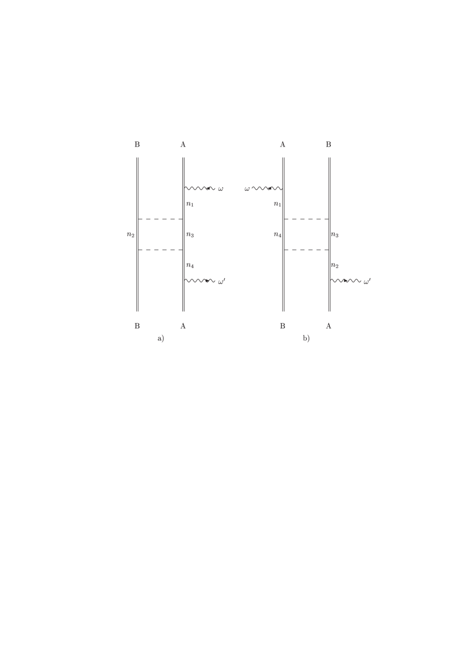
Figure 18: The Feynman graphs that describe the exchange by two Coulomb photons between atomic electrons in the process of elastic photon scattering on an atom.

The next iteration with respect to the Coulomb interaction $V_{\rm{C}}$ follows from the graph in Fig. 18. In this case the resonance approximation implies that $n_{1},n_{4}=A$ and $n_{2},n_{3}\in A^{\prime},B$. The inclusion of all possible combinations leads to the correction

$$U_{\rm{em}}=\frac{(U^{*}_{\omega})_{AA^{\prime}}}{E_{A^{\prime}}-E_{A}-\omega}\,\frac{\left[(V_{\rm{C}})_{A^{\prime}B;A^{\prime}B}\right]^{2}}{(E_{A^{\prime}}-E_{A}-\omega)^{2}}\,.$$ (112)

An all-order resummation of the iterations results in a geometric progression and thus in an energy shift in the denominator

$$U_{\rm{em}}=\frac{(U^{*}_{\omega})_{AA^{\prime}}}{E_{A^{\prime}}+\Delta E^{c1}_{A^{\prime}B}-E_{A}-\omega}\,.$$ (113)

Here $\Delta E^{c1}_{A^{\prime}B}$ is the first-order Coulomb IIC:

$$\Delta E^{c1}_{A^{\prime}B}=(V_{\rm{C}})_{A^{\prime}B;A^{\prime}B}\,.$$ (114)

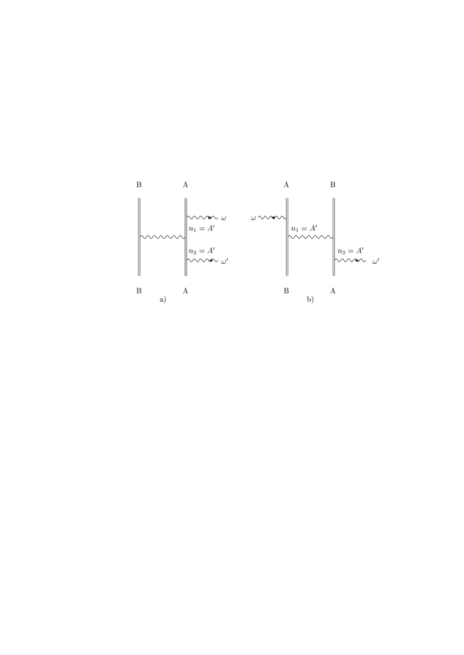
Figure 19: Feynman graphs that describe the elastic photon scattering on the two-electron ion in resonance approximation with the first-order Breit interelectron interaction corrections taken into account. The wavy internal line denotes the Breit (transverse) photon. The other notations are the same as in Fig. 17.

Exactly the same derivation can be repeated for the Breit interaction leading to the expression (see Fig. 19):

$$U_{\rm{em}}=\frac{(U^{*}_{\omega})_{AA^{\prime}}}{E_{A^{\prime}}+\Delta E^{1}_{A^{\prime}B}-E_{A}-\omega}\,,$$ (115)

where

$$\Delta E^{1}_{A^{\prime}B} =\Delta E^{C1}_{A^{\prime}B}+\Delta E^{B1}_{A^{\prime}B},$$ (116)

$$\Delta E^{B1}_{A^{\prime}B} =(V_{\rm{B}})_{A^{\prime}B;A^{\prime}B}.$$ (117)

The matrix elements of the Breit interaction $V_{\rm{B}}$ are defined as:

$$(V_{\rm{B}})_{A^{\prime}BA^{\prime}B} =-e^{2}\left(\frac{\alpha_{i_{1}}\alpha_{i_{2}}}{r_{12}}\right)_{A^{\prime}BA^{\prime}B}\,,$$ (118)

$$(V_{B})_{BA^{\prime}A^{\prime}B} =e^{2}\left(\frac{\alpha_{i_{1}}\alpha_{i_{2}}-1}{r_{12}}e^{i|E_{A^{\prime}}-E_{B}|r_{12}}\right)_{BA^{\prime}A^{\prime}B}\,.$$ (119)

Here $\alpha_{i_{1}},\alpha_{i_{2}}$ denote the Dirac matrices which act on one-electron wave functions depending on spatial variables $\vec{x}_{1},\vec{x}_{2}$ and $i=1,2,3$ .

Moreover, we can perform simultaneously the resummation of the radiative insertions in the electron propagator. According to the derivations presented in section 3, this yields the result

$$U_{\rm{em}}=\frac{(U^{*}_{\omega})_{AA^{\prime}}}{\tilde{E}_{A^{\prime}}+\Delta E^{1}_{A^{\prime}B}-E_{A}-\omega}\,.$$ (120)

The emission line profile can now be expressed, as described in section 4.

Following the derivations of section 5 we account for the higher-order IIC as well. For example the second-order Coulomb-Coulomb IIC can be obtained from Fig. 18 for $n_{1},n_{4}=A^{\prime}$ but $n_{2},n_{3}\bar{\in}A^{\prime},B$. The part of this graph containing two Coulomb interactions can now be considered as a complicated insertion into the electron line corresponding to the state $A$. Repeating these insertions and summing up the resulting geometric progression we shall obtain an additional shift in the denominator that will represent exactly the second-order Coulomb-Coulomb IIC. Similar manipulations can be performed for the second-order Coulomb-Breit and Breit-Breit IIC. In the two latter cases reducible contributions also arise due the dependence of the IIC corrections on the photon frequency $\omega$ [24], [48], [49].

These reducible contributions, i.e., the so-called reference-state contributions or derivative contributions can be obtained in the same manner as the reducible contributions discussed in section 5.

The derivation of the IIC correction to the emission amplitude follows to the derivation of the radiative correction presented in section 6. Assuming now that in Fig. 17 and Fig. 19 $n_{1}\neq A^{\prime}$ but $n_{2}=A^{\prime}$ and that all previous insertions are also performed as well, we obtain the generalization of Eq. (120)

$$U_{\rm{em}}=\frac{(U^{*}_{\omega})_{A\tilde{A}^{\prime}}}{\tilde{E}_{A^{\prime}}+\Delta E^{1}_{A^{\prime}B}-E_{A}-\omega}\,.$$ (121)

Here

$$(U^{*}_{\omega})_{A\tilde{A}^{\prime}}=\sum_{n_{1}\neq A^{\prime}}\frac{(U^{*}_{\omega})_{An_{1}}\left[(V_{\rm{C}})_{Bn_{1};BA^{\prime}}+(V_{\rm{B}})_{Bn_{1};BA^{\prime}}\right]}{E_{n_{1}}-E_{A^{\prime}}}$$ (122)

is the first-order IIC to the emission matrix element (correction to the wave function of the state $A^{\prime}$).

To obtain the shift of the energy $E_{A}$ in the denominator of Eq. (121), as well as the correction to the wave function $\Psi_{A}$ in the emission matrix element we have to turn over again to the double resonance photon scattering picture as described in section 12. The following section will be devoted to this issue.

17 Double photon scattering on two-electron ions

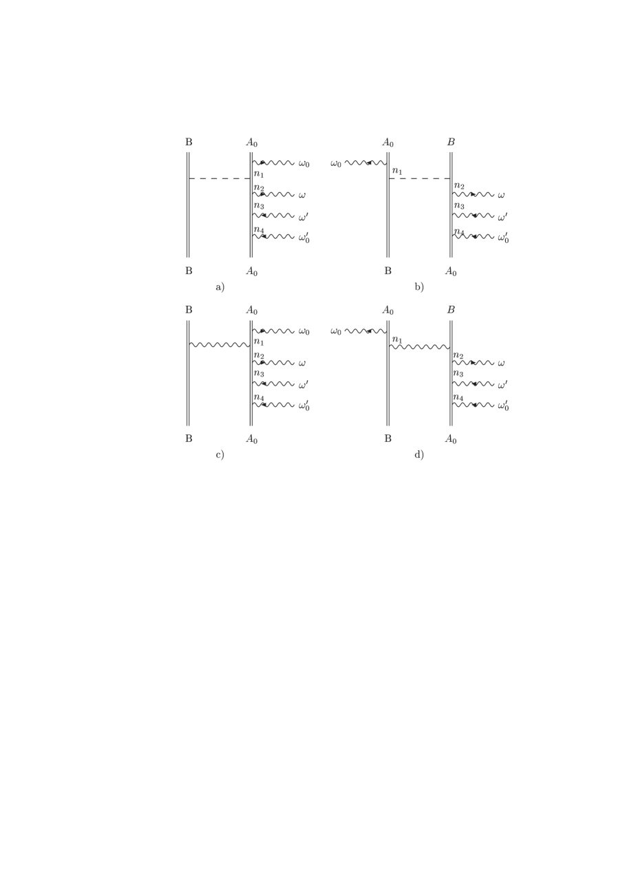
Figure 20: Feynman graphs that describe interelectron interaction first-order insertions: a), b) correspond to the Coulomb ”direct” and ”exchange” graphs; c), d) correspond to the Breit ”direct” and ”exchange” graphs.

The double photon resonant scattering process described in section 7 can be applied without any modifications to two-electron ions. The first-order IIC insertions into the central electron propagator in Fig. 5 will yield as was shown in section 8 for the radiative insertions the same result that was already obtained with the single photon scattering: the shift of the energy $E_{A^{\prime}}$ in the Lorentz denominator and the correction to the wave function $\Psi_{A^{\prime}}$ in the emission matrix element. Instead of repeating this derivation we start with the IIC insertions into the upper electron propagator in Fig. 5. These insertions to first order are shown in Fig. 20. Applying similar steps as described in section 9, we derive an expression for the double photon emission amplitude

$$U_{\rm{em}}=\frac{(U^{*}_{\omega_{0}})_{A_{0}A}(U^{*}_{\omega})_{AA^{\prime}}}{(\tilde{E}_{A}+\Delta E^{1}_{AB}-E_{A_{0}}-\omega)(\tilde{E}_{A^{\prime}}+\Delta E^{1}_{A^{\prime}B}-E_{A_{0}}-\omega_{0}-\omega)}\,.$$ (123)

For obtaining Eq. (123) we have set $n_{1}=n_{2}=A,n_{3}=A^{\prime},n_{4}=A$ in the diagrams Fig. 20 a)-d). We can also generalize Eqs. (60), (61) for the Lorentz line profile both for the excited and for the ground state $A$. The only difference to Eqs. (60), (61) is that now the frequency $\tilde{\omega}_{A^{\prime}A}$ also accounts for the IIC

$$\tilde{\omega}_{A^{\prime}A(B)}=\tilde{E}_{A}+\Delta E_{AB}-\tilde{E}_{A^{\prime}}-\Delta E_{A^{\prime}B}\,.$$ (124)

Such interelectronic interaction corrections can be of any order

$$\Delta E_{AB}=\sum_{i=1}^{\infty}\Delta E^{i}_{AB}$$ (125)

and the same holds true for $\Delta E_{A^{\prime}B}$.

Accordingly we can replace $\tilde{\omega}_{A^{\prime}A(B)}$ by its experimental value $\omega^{\rm{exp}}_{A^{\prime}A(B)}$. This is especially important for two-electron ions, where the energy differences between the levels within a multiplet can be deduced experimentally more accurately, than from theory.

Finally, we can write down the correction to the emission matrix element (to the wave function of the state $A$), following derivations presented in section 11

$$U_{\rm{em}}=\frac{(U^{*}_{\omega_{0}})(U^{*}_{\omega})_{\tilde{A}A^{\prime}}}{(\tilde{E}_{A}+\Delta E_{AB}-E_{A_{0}}-\omega_{0})(\tilde{E}_{A^{\prime}}+\Delta E_{A^{\prime}B}-E_{A_{0}}-\omega_{0}-\omega)}\,,$$ (126)

where

$$(U^{*}_{\omega})_{\tilde{A}A^{\prime}}=\sum_{n_{2}\neq A}\frac{\left[(V_{\rm{C}})_{BA;Bn_{2}}+(V_{\rm{B}})_{BA;Bn_{2}}\right](U^{*}_{\omega})_{n_{2}A^{\prime}}}{E_{n_{2}}-E_{A}}\,.$$ (127)

For deriving Eq. (127) we have set $n_{1}=A,n_{3}=A^{\prime},n_{4}=A,$ but now with $n_{2}\neq A$ in Figs. 20 a)-d).

Again we can write down all the corrections to the transition probability $A^{\prime}B\rightarrow AB$ (or the partial width $\Gamma_{AB;A^{\prime}B}$) in the form of Eq. (65).

The first-order IIC to the transition probability can be always represented by the sum

$$\Gamma_{AB,A^{\prime}B}=\Gamma_{AA^{\prime}}+\Gamma_{\tilde{A}A^{\prime}}+\Gamma_{A\tilde{A}^{\prime}}$$ (128)

where $\Gamma^{(B)}_{\tilde{A}(B)A^{\prime}}$ and $\Gamma^{C}_{A\tilde{A}^{\prime}(B)}$ represent one-electron partial widths with improved amplitudes given by Eqs. (122) and (127), respectively.

18 The interelectron interaction corrections to the weak interaction amplitude

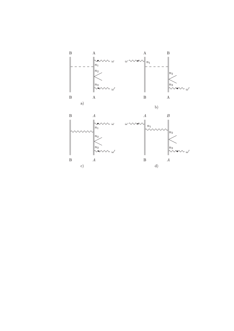
Figure 21: Feynman graphs that describe the weak interaction-admixed amplitude of photon scattering on two-electron ions. The graphs a), b) correspond to the interelectron interaction first-order Coulomb ”direct” and ”exchange” insertions, the graphs c), d) correspond to ”direct” and ”exchange” Breit insertions.

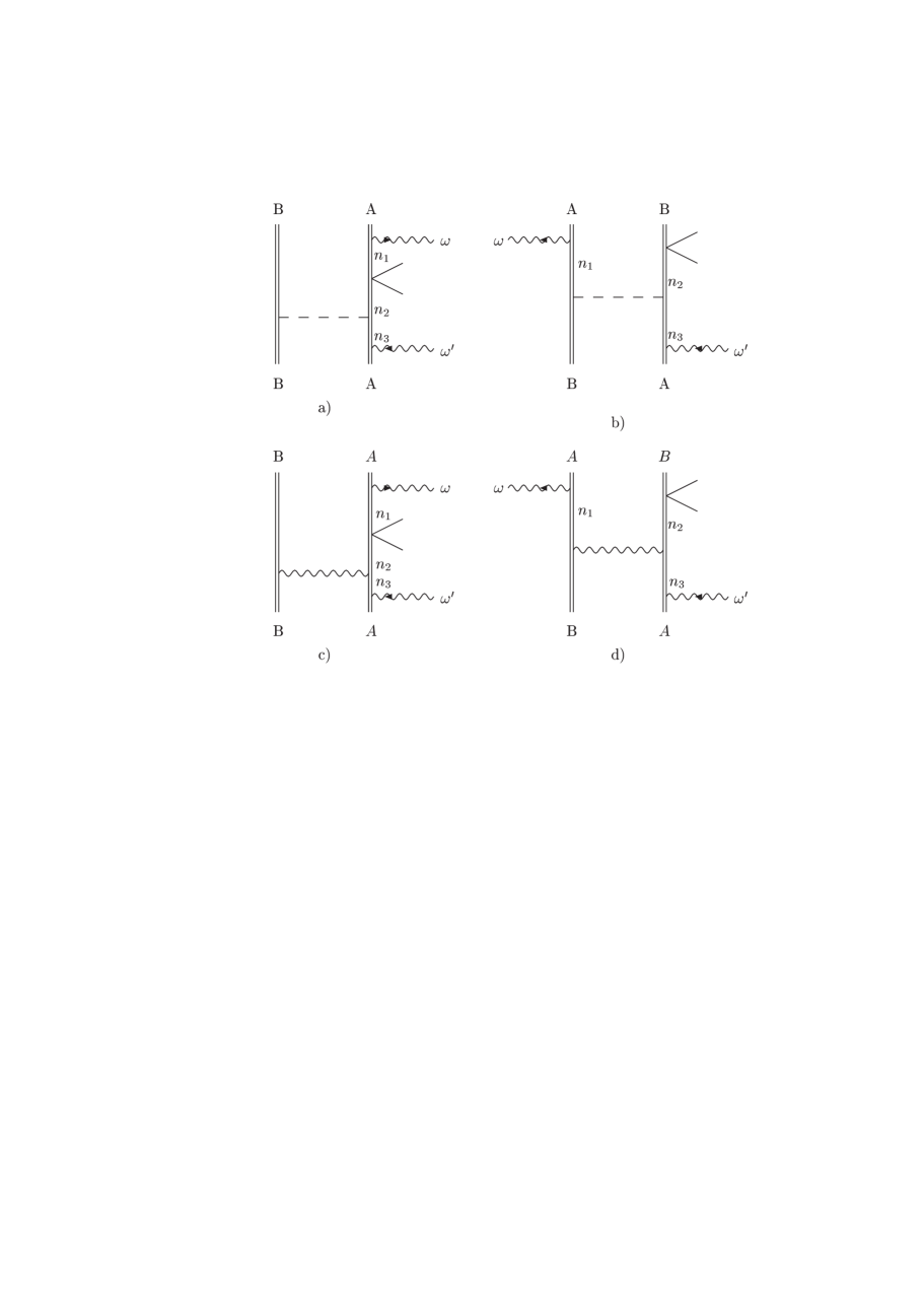
Figure 22: Feynman graphs that describe the weak interaction-admixed amplitude of the photon scattering on two-electron ions. Unlike the graphs in Fig. 21 that correspond to interelectron interaction corrections insertions to the upper electron propagator in Fig. 10, Fig. 22 corresponds to the interelectron interaction insertions in the lower propagator.

To evaluate the IIC corrections to the weak interaction amplitude we can take the sections 13-14 as a guide-line. The generalization of the diagrams in Fig. 10 to two-electron ions with IIC insertions into the electron propagators is depicted in Figs. 21 and 22.

Consider first the IIC in Fig. 21. Here we take $n_{3}=E_{A^{\prime}}$ (resonant case) and $n_{1}=n_{2}=E_{A^{\prime\prime}}$ (dominant state). Then the summation of IIC insertions to all orders will result in (compare with Eq. (88))

$$U_{\rm{em}}=\frac{(U^{*}_{\omega})_{AA^{\prime\prime}}}{\tilde{E}_{A^{\prime\prime}}+\Delta E_{A^{\prime\prime}B}-E_{A}-\omega}\,\frac{(\gamma_{0}V_{\rm{PNC}})_{A^{\prime\prime}A^{\prime}}}{\tilde{E}_{A^{\prime}}-E_{A}-\omega}\,.$$ (129)

We assume that the radiative insertions are already performed. If $n_{2}\neq A^{\prime\prime}$ we obtain the correction to the PNC matrix element (to the wave function $\Psi_{A^{\prime\prime}}$)

$$U_{\rm{em}}=\frac{(U^{*}_{\omega})_{AA^{\prime\prime}}}{\tilde{E}_{A^{\prime\prime}}+\Delta E_{A^{\prime\prime}B}-E_{A}-\omega}\frac{(\gamma_{0}V_{\rm{PNC}})_{\tilde{A}^{\prime\prime}A^{\prime}}}{\tilde{E}_{A^{\prime}}-E_{A}-\omega}\,,$$ (130)

where

$$(\gamma_{0}V_{\rm{PNC}})_{\tilde{A}^{\prime\prime}A^{\prime}}=\sum_{n_{2}\neq A^{\prime\prime}}\frac{\left[(V_{\rm{C}})_{BA^{\prime\prime};Bn_{2}}+(V_{\rm{B}})_{BA^{\prime\prime};Bn_{2}}\right](\gamma_{0}V_{\rm{PNC}})_{n_{2}A^{\prime}}}{E_{n_{2}}-E_{A^{\prime\prime}}}\,.$$ (131)

For the IIC in Fig. 22 we have to choose the dominant state $n_{1}=A^{\prime\prime}$ and the resonant states $n_{1}=n_{2}=A^{\prime}$. Then the summation of IIC insertions to all orders yields (assuming again that the summation in Fig. 21 is already performed)

$$U_{\rm{em}}=\frac{(U^{*}_{\omega})_{AA^{\prime\prime}}}{\tilde{E}_{A^{\prime\prime}}+\Delta E_{A^{\prime\prime}B}-E_{A}-\omega}\,\frac{(\gamma_{0}V_{\rm{PNC}})_{A^{\prime\prime}A^{\prime}}}{\tilde{E}_{A^{\prime}}+\Delta E_{A^{\prime}B}-E_{A}-\omega}\,.$$ (132)

As in section 14 we employ the resonance condition $\omega=\tilde{E}_{A^{\prime}}+\Delta E_{A^{\prime}B}-E_{A}$ obtained from the second denominator in Eq. (132) and insert it into the first denominator:

$$U_{\rm{em}}=\frac{(U^{*}_{\omega})_{AA^{\prime\prime}}}{\tilde{E}_{A^{\prime\prime}}+\Delta E_{A^{\prime\prime}B}-\tilde{E}_{A^{\prime}}-\Delta E_{A^{\prime}B}}\,\frac{(\gamma_{0}V_{\rm{PNC}})_{A^{\prime\prime}A^{\prime}}}{\tilde{E}_{A^{\prime}}+\Delta E_{A^{\prime}B}-E_{A}-\omega}\,.$$ (133)

The meaning of ”dominant” state for two-electron ions needs to be clarified. These states should now be specified in a different manner compared to one-electron ions. The most advantageous situation for the observation of the effects in two-electron ions occurs when two levels belonging to the same multiplet but possessing opposite parity appear to be nearly degenerated. Unlike in the case of one-electron ions in two-electron ions this can happen only accidentally. The standard example is the crossing of the $1s2s{}^{1}S_{0}$ and $1s2p{}^{3}P_{0}$ levels that occurs for $Z$ = 6 (carbon), $Z$ = 64 (gadolinium) and $Z$ = 92 (uranium) He-like ions [25]- [29]), [31].

Introducing the frequency

$$\tilde{\omega}_{A^{\prime\prime}A^{\prime}(B)}=\tilde{E}_{A^{\prime\prime}}+\Delta E_{A^{\prime\prime}B}-\tilde{E}_{A^{\prime}}-\Delta E_{A^{\prime}B}$$ (134)

we may replace it then by the experimental value $\tilde{\omega}^{\rm{exp}}_{A^{\prime\prime}A^{\prime}(B)}$. The exact theoretical value for the splitting $\tilde{\omega}_{A^{\prime\prime}A^{\prime}(B)}$ between the nearly degenerated levels of the two-electron ions can be also used. Now the energy difference $\tilde{\omega}_{A^{\prime\prime}A^{\prime}(B)}$ plays the role of the small denominator $\Delta E_{L}$ and we can write down the analogue of Eq. (95) in the form

$$U_{\rm{em}}=\frac{(U^{*}_{\omega})_{AA^{\prime\prime}}}{\tilde{E}_{A^{\prime}(B)}-E_{A}-\omega}\,\frac{(\gamma_{0}V_{\rm{PNC}})_{A^{\prime\prime}A^{\prime}}}{\Delta E_{L}}$$ (135)

where $\Delta E_{L}=\tilde{\omega}_{A^{\prime\prime}A^{\prime}(B)}$ and

$$\tilde{E}_{A^{\prime}(B)}=\tilde{E}_{A^{\prime}}+\Delta E_{A^{\prime}B}\,.$$ (136)

Setting now $n_{2}\neq A^{\prime}$ in Fig. 22 we obtain the correction to the PNC matrix element (to the wave function in the state $A^{\prime}$)

$$U_{\rm{em}}=\frac{(U^{*}_{\omega})_{AA^{\prime\prime}}}{\tilde{E}_{A^{\prime}(B)}-E_{A}-\omega}\,\frac{(\gamma_{0}V_{\rm{PNC}})_{A^{\prime\prime}\tilde{A}^{\prime}}}{\Delta E_{L}}\,,$$ (137)

where

$$(\gamma_{0}V_{\rm{PNC}})_{A^{\prime\prime}\tilde{A}^{\prime}}=\sum_{n_{2}\neq A^{\prime}}\frac{(\gamma_{0}V_{\rm{PNC}})_{A^{\prime\prime}n_{2}}\left[(V_{\rm{C}})_{Bn_{2};BA^{\prime}}+(V_{\rm{B}})_{Bn_{2};BA^{\prime}}\right]}{E_{n_{2}}-E_{A^{\prime}}}\,.$$ (138)

The similar replacement $\tilde{E}_{A^{\prime\prime}(B)}-E_{A}-\omega\rightarrow\Delta E_{L}$ can be made in Eq. (130).

Again we do not consider the graphs with $V_{\rm{PNC}}$ inserted in the outer electron lines, since they do not contain any small denominators $\Delta E_{L}$.

Finally, we end up with an expression for the PNC matrix element with all the IIC taken into account

$$(\gamma_{0}V_{\rm{PNC}})_{A^{\prime\prime}A^{\prime}}=(\gamma_{0}V_{\rm{PNC}})_{A^{\prime\prime}A^{\prime}}+(\gamma_{0}V_{\rm{PNC}})_{A^{\prime\prime}\tilde{A}^{\prime}}+(\gamma_{0}V_{\rm{PNC}})_{\tilde{A}^{\prime\prime}A^{\prime}}\,,$$ (139)

where the corrected matrix elements $(\gamma_{0}V_{\rm{PNC}})_{A^{\prime\prime}\tilde{A}^{\prime}}$ and $(\gamma_{0}V_{\rm{PNC}})_{\tilde{A}^{\prime\prime}A^{\prime}}$ are defined by Eqs. (138) and (131), respectively.

19 The interelectron interaction corrections in the Dirac-Hartree-Fock approximation

The QED theory of highly-charged ions, based on the Dirac-Hartree-Fock (DHF) taken as zero-order approximation has been considered in [3]. Due to the energy dependence in the Breit-interaction matrix elements (see Eq. (119)), the Breit-interaction cannot be included exactly in the zero-order DHF scheme. Therefore, we will consider here the DHF approximation restricting to the Coulomb interaction only and leaving the Breit interaction to be accounted perturbatively. Nevertheless, we may emphazise that the DHF method together with an approximate inclusion of the Breit interaction is widely used and leads to very accurate results even for high-$Z$ ions (see, for example [11]).

In DHF approximation the one-electron equation (1) should be replaced by

$$(\not{p}-m+\gamma_{0}eV+\gamma_{0}eV_{\rm HF})\Psi=0$$ (140)

where the operator $V_{\rm{HF}}$ is defined as

$$V_{\rm{HF}}(\vec{r}\,)f(\vec{r}\,)=\sum^{N}_{m=1}\int\,d\,^{3}r^{\prime}\,\Psi^{+}_{m}({\vec{r}}\,^{\prime})V_{\rm{C}}(\vec{r},{\vec{r}}\,^{\prime})\Psi_{m}({\vec{r}}\,^{\prime})f(\vec{r}\,)\\ -\sum^{N}_{m=1}\int\,d\,^{3}r\,\Psi^{+}_{m}({\vec{r}}\,^{\prime})V_{\rm C}(\vec{r},\vec{r}\,^{\prime})f({\vec{r}}\,^{\prime})\Psi_{m}(\vec{r}\,)\,.$$ (141)

In Eq. (141) $\Psi_{m}(\vec{r}\,)$ are the solutions of the DHF equation with eigenvalues $E_{m},f(\vec{r}\,)$ is an arbitrary 4-component spinor function and the summation is extended to all occupied states of the $N$-electron atom or ion.

For highly-charged ions we can consider the term $\gamma_{0}V_{\rm{HF}}$ in Eq. (140) as a perturbation. Then the first-order correction to the Coulomb wave function $\Psi_{A}$ (the solution of Eq. (1)) will read

$$\Psi^{1}_{A}(\vec{r}\,)=\sum_{n\neq A}\frac{(V_{\rm{HF}})_{nA}}{E_{n}-E_{A}}\Psi_{n}(\vec{r}\,)\,.$$ (142)

Using the definition of the operator $V_{\rm{HF}}$, we obtain

$$\Psi^{1}_{A}(\vec{r}\,)=\sum^{N}_{m=1}\sum_{n\neq A}\frac{(V_{C})_{nm;Am}\Psi_{n}(\vec{r}\,)}{E_{n}-E_{A}}\,.$$ (143)

In case of two-electron ions the sum over $m$ in Eq. (143) reduces to one term $m=B$. Then, we obtain the corrections $(U^{*}_{\omega})_{A\tilde{A}^{\prime}}$ and $(U^{*}_{\omega})_{\tilde{A}A^{\prime}}$ to the emission matrix element (Eqs. (122) and (127) only with the Coulomb potential $V_{\rm{C}}$) if we replace the corrected wave functions $\Psi_{\tilde{A}}$ and $\Psi_{\tilde{A}^{\prime}}$ by the expression (143). This means that when evaluating the emission matrix elements with DHF functions we will automatically take into account the corrections Eq. (122) and Eq. (127) with the Coulomb operator. The DHF functions include also higher-order Coulomb corrections which are negligible for high-$Z$ values. The same holds true for the corrections to the PNC matrix elements as given by Eqs. (131) and (138), respectively.

20 Conclusions

Summarizing the results obtained in the present paper we can state that a most general QED approach has been elaborated for the evaluation of various spectroscopical properties of highly-charged ions: energy level shifts, transition rates and line profiles. The physical process of photon scattering on atomic electrons provides a proper basis for rigorous QED evaluations of all quantities being of current interest in studies of highly charged ions.

The resonance approximation has been proven to be a powerful tool for obtaining nonperturbative results such as the energy shifts in the Lorentz denominators. This is a most physical way to determine the atomic energy shifts.

Rigorous QED expressions for all generic radiative corrections to the photon emission process are presented including simultaneously the radiative shift of the Lorentz denominator. Thus a full QED treatment of the Lorentz profile is achieved. The weak interaction-induced parity violating amplitudes are also treated within this approach and a closed expression for radiative corrections to the PNC matrix element has been derived. This allows for future accurate calculations of the PNC effect in highly charged ions. Furthermore, the theory is extended also to few-electron ions.

QED and PNC corrections to the emission amplitude are presented for the most interesting case of single-excited states in two-electron ions. The renormalization procedure for both pure QED radiative corrections and QED corrections in the presence of a parity-violating effective potential is discussed and the cancellation of the infrared divergencies is verified.

The general QED approach and the formulas for the various QED corrections derived in the paper provide a firm theoretical basis for numerical calculations in the near future.

Figure 1: Feynman graph describing the elastic photon scattering on an atomic electron. The double solid line denotes the bound electron in the field of the nucleus. The wavy lines with the arrows denote the photon emission and absorption. The indices A, n correspond to the initial (final) and intermediate states.

Figure 2: Feynman graph corresponding to the electron self-energy insertions into the electron propagator in graph Fig. 1. The notations are the same as in Fig. 1.

Figure 3: Feynman graph corresponding to double self-energy insertions in the resonance approximation.

Figure 5: Feynman graph describing the elastic scattering of two photons on an atomic electron in the state $A_{0}$.

Figure 7: Feynman graph corresponding to self-energy insertions in the upper electron propagator in Fig. 5.

Figure 11: The self-energy insertion in the upper electron propagator in Fig. 10.

Figure 12: The self-energy insertions in the lower electron propagator in Fig. 10

Figure 13: Feynman graph describing the self-energy electromagnetic vertex correction to the weak amplitude in Fig. 10.

Figure 14: Feynman graphs describing the vacuum polarization electromagnetic vertex correction to the weak amplitude in Fig. 10: a) exact expression b) Uehling approximation.

References

-
[1]
Th. Stöhlker, P. H. Mokler, F. Bosch, R. W. Dunford,
F. Franzke, O. Klepper, C. Kozhuharov, T. Ludziejewski,
F. Nolden, H. Reich, P. Rymuza, Z. Stachura, M. Steck,
P. Swiat and A. Warczak, Phys. Rev. Lett. 85, (2000) 3109;
P. H. Mokler, Hyperfine Interactions 114, (1998) 21 ;
P. Seelig, A. Dax, S. Faber, M. Gerlack, G. Huber, T. Kühl, D. Marx, P. Merz, W. Quint, F. Schmidt, H. Winter and M. Würtz, Hyperfine Interactions 114, (1998) 135;
P. Beiersdorfer, A. L. Osterfeld, J. H. Scofield, J. R. Crespo-Lopez-Urrutia and K. Widmann, Phys. Rev. Lett. 80, (1998) 3022. -
[2]
R. Marrus, A. Simionovici, P. Indelicato, D. D. Dietrich,
P. Charles, J.-P. Briand, K. Finlayson, F. Bosh, D. Liesen and
F. Parente, Phys. Rev. Lett. 63, (1989) 502;
R. W. Dunford, C. J. Liu, J. Last, N. Berrah-Mansour, R. Vondrasek, D. A. Church and L. J. Curtis, Phys. Rev. A 44, (1991) 764;
B. B. Birkett, J. -P. Briand, P. Charles, D. D. Dietrich, K. Finlayson, P. Indelicato, D. Liesen, R. Marrus and A. Simionovic, Phys. Rev. A 47, (1993) R2454;
A. Simionovici, B. B. Birkett, J. -P. Briand, P. Charles, D. D. Dietrich, K. Finlayson, P. Indelicato, D. Liesen and R. Marrus, Phys. Rev. A 48, (1993) 1695. - [3] L. N. Labzowsky, G. L. Klimchitskaya and Yu. Yu. Dmitriev, in ”Relativistic Effects in the Spectra of Atomic System”, IOP Publishing, Bristol, 1993.
- [4] P. J. Mohr, G. Plunien and G. Soff, Phys. Rep. 293, (1998) 227.
- [5] T. Beier, Phys. Rep. 339, (2000) 79.
- [6] V. Shabaev, Phys. Rep. 356, (2002) 119.
- [7] R. Marrus and P. Mohr, Adv. in At. and Mol. Phys. 14, (1978) 181.
- [8] P. Beiersdorfer, A. L. Osterfeld and S. R. Elliott, Phys. Rev. A 58, (1988) 1944.
- [9] W. R. Johnson and C. D. Lin, Phys. Rev. 14, (1976) 565.
- [10] G. W. F. Drake, Phys. Rev. A 19, (1979) 1387.
- [11] W. R. Johnson, D. Plante and J. Sapirstein, Adv. in At. Mol. Phys. 46, (1995) 556.
- [12] V. M. Shabaev, J. Phys. A 24, (1991) 5665.
- [13] V. Weisskopf and E. Wigner, Z. Phys. 63, (1930) 54.
- [14] F. Low, Phys. Rev. 88, (1951) 53.
- [15] L. N. Labzowsky, Zh. Eksp. Teor. Fiz. 85, (1983) 869.
- [16] L. N. Labzowsky, J. Phys. B 26, (1993) 1039.
- [17] V. G. Gorshkov, L. N. Labzowsky and A. A. Sultanaev, Zh. Eksp. Teor. Fiz. 96, (1989) 53 [Engl. Transl. Sov. Phys. JETP 69, (1989) 28].
- [18] V. V. Karasiev, L. N. Labzowsky, A. V. Nefiodov, V. G. Gorshkov and A. A. Sultanaev, Phys. Scr. T 46, (1992) 225
- [19] L. N. Labzowsky, V. V. Karasiev and I. Goidenko, J. Phys B 27, (1994) L439.
- [20] L.N. Labzowsky, I. Goidenko and D. Liesen, Phys. Scr. 56, (1997) 271.
- [21] L. N. Labzowsky, D. A. Solovyov, G. Plunien and G. Soff, Phys. Rev. Lett. 87, (2001) 143003.
- [22] L. N. Labzowsky, V. Karasiev, I. Lindgren, H. Persson and S. Salomonson, Phys. Scr. T 46, (1993) 150
- [23] L. N. Labzowsky, M. A. Tokman, Adv. Quant. Chem. 30, (1998) 393.
- [24] O. Yu. Andreev, L. N. Labzowsky, G. Plunien and G. Soff, Phys. Rev. A 64, (2001) 042513
- [25] V. G. Gorshkov and L. N. Labzowsky, Pis’ma Zh. Eksp.Teor. Fiz. 19, (1974) 768 [Engl. Transl. JETP Lett. 19, (1974) 394].
- [26] A. Schäfer, G. Soff, P. Indelicato, B. Müller and W. Greiner, Phys. Rev. A 40, (1989) 7362.
- [27] G. von Oppen, Z. Phys. D 21, (1981) 181.
- [28] V. V. Karasiev, L. N. Labzowsky and A. V. Nefiodov, Phys. Lett. A 172, (1992) 62.
- [29] R. W. Dunford, Phys. Rev. A 54, (1996) 3820.
- [30] M. Zolotorev and D. Budker, Phys. Rev. Lett. 78, (1997) 4717.
- [31] L. N. Labzowsky, A. V. Nefiodov, G. Plunien, G. Soff, R. Marrus and D. Liesen, Phys. Rev. A 63, (2001) 054105.
- [32] I. Bednyakov, L. N. Labzowsky, G. Plunien, G. Soff and V. Karasiev, Phys. Rev. A 61, (1999) 012103
- [33] P. J. Mohr, Ann. Phys. (N.Y.) 88, (1974) 26.
- [34] U. D. Jentschura, P. J. Mohr and G. Soff, Phys. Rev. A 63, (2001) 042512.
- [35] H. Persson, I. Lindgren and S. Salomonson, Phys. Scr. T 46, (1993) 125.
- [36] H. M. Quiney and I. P. Grant, Phys. Scr. T 46, (1993) 132.
- [37] L. Labzowsky, I. Goidenko and A. Nefiodov, J. Phys. B 31, (1998) L477.
- [38] Yu. Dmitriev, T. Fedorova and D. Bogdanov, Phys. Lett. A 241, (1998) 84.
- [39] E. A. Uehling, Phys. Rev. 48, (1935) 55.
- [40] L. N. Labzowsky, A. O. Mitrushenkov, Phys. Rev. A 53, (1996) 3029.
- [41] E. Lifshits, L. Landau and L. Pitajevskii, “Quantum Electrodynamics”, Pergamon Press, London-Paris, 1983.
- [42] C. Caso et al., Eur. Phys. J. C 3, (1998) 1.
- [43] S. Blundell, P. J. Mohr, W. R. Johnson and J. Sapirstein, Phys. Rev. A 48, (1993) 2615.
- [44] I. Lindgren, H. Persson, S. Salomonson and L. Labzowsky, Phys. Rev. A 51, (1995) 1167.
- [45] V. A. Yerokhin, A. N. Artemyev, V. M. Shabaev, M. M. Sysak, O. M. Zherebtsov and G. Soff, Phys. Rev. Lett. 85, (2000) 4699.
- [46] V. A. Yerokhin, A. N. Artemyev, V. M. Shabaev, M. M. Sysak, O. M. Zherebtsov and G. Soff, Phys. Rev. A 64, (2001) 032109
- [47] P. J. Mohr and J. Sapirstein, Phys. Rev. A 62, (2000) 052501.
- [48] L. N. Labzowsky and M. A. Tokman, J. Phys. B 28, (1995) 3717.
- [49] L. N. Labzowsky and M. A. Tokman, Adv. Quant. Chem. 30, (1998) 393.