Understanding highly excited states via parametric variations

Abstract

Highly excited vibrational states of an isolated molecule encode the vibrational energy flow pathways in the molecule. Recent studies have had spectacular success in understanding the nature of the excited states mainly due to the extensive studies of the classical phase space structures and their bifurcations. Such detailed classical-quantum correspondence studies are presently limited to two or quasi two dimensional systems. One of the main reasons for such a constraint has to do with the problem of visualization of relevant objects like surface of sections and Wigner or Husimi distributions associated with an eigenstate. This necessiates various alternative techniques which are more algebraic than geometric in nature. In this work we introduce one such method based on parametric variation of the eigenvalues of a Hamiltonian. It is shown that the level velocities are correlated with the phase space nature of the corresponding eigenstates. A semiclassical expression for the level velocities of a single resonance Hamiltonian is derived which provides theoretical support for the correlation. We use the level velocities to dynamically assign the highly excited states of a model spectroscopic Hamiltonian in the mixed phase space regime. The effect of bifurcations on the level velocities is briefly discussed using a recently proposed spectroscopic Hamiltonian for the HCP molecule.

I Introduction

Determining the nature of the highly excited rovibrational states is important in the context of unraveling the intramolecular vibrational energy redistribution (IVR) pathways in moleculesrev1 ; rev2 ; rev3 ; rev4 ; rev5 ; rev6 ; rev7 . At high energies the usual rigid rotor-harmonic oscillator descriptions are inadequate due to the breakdown of the normal mode approximation. The various normal modes get coupled leading to complicated spectra and patterns. The underlying classical phase space usually has a mixed character i.e., regular regions interspersed with the chaotic regions. The mixed nature of the phase space gives rise to a variety of phenomena, classicaluzer and quantumtun , which in turn lead to complex spectral patterns in terms of the intensities and splittings.

Much of the recent workwater ; water1 ; ethy ; chbr ; dco ; annu ; jpc on small polyatomic molecules has clearly shown that the underlying classical dynamics plays a significant role in determining the nature of the highly excited states. In particular, the various classical phase space structures like periodic orbits, resonance zones and effects like bifurcationsjpc ; kell leave their imprints on the eigenstates and hence provide important clues to IVR. Almost all of the work has been constrained to atmost two degrees of freedom systems. One of the main reasons for such a constraint have to do with the fact that visualizing the classical phase space structures, for that matter even the quantum states, is quite involved for systems with more than two degrees of freedom. Moreover, determining the relevant periodic orbitsfarant and higher dimensional objects like resonant 2-tori becomes difficult as the number of degrees of freedom increases. It is obvious that studying IVR in large molecules from such useful classical-quantum correspondence viewpoints would require one to come up with dimensionality independent techniques. Although not the focus of the present work, it is important to note that novel dynamical phenomena like Arnol’d diffusionarnold and complex instabilitycinst arise in systems with dimensionality greater than two. It remains to be seen wether such effects have important consequences for the classical-quantum correspondence studies of highly excited states and hence IVR.

In principle, once the detailed phase space structure is at hand, the required information can be extracted by correlating with a phase space representation of the quantum states, like the Husimihus or the Wignerwig distributions. However, given that a detailed classical phase space study of even three degree of freedom systems is sparsenato ; licht ; ccm ; mde ; lask suggests that the straightforward approach is far from easy. Ideally one would like a method that yields the required information in a basis independent fashion without the need to explicitly determine the classical periodic orbits, to visualize the surface of sections and then comparing to the relevant phase space distributions. The search for such a method, if it exists, seems to be rather difficult at the present moment. In this work we attempt to provide a first step towards such an important yet difficult goal.

The above mentioned factors clearly indicate that one needs algebraic measures that would unambigously provide the information on the nature of the eigenstates. To this end certain measures, time dependent and independent, have been proposed in the literature. For instance, inverse participation ratiosipr (IPR) or dilution factors can yield information about the nature of the localization of the eigenstates. However IPR is a basis dependent quantity and cannot provide information about the invariant classical structures relevant to the eigenstate. It is possible to extract useful information by computing the IPR in different basis which are optimal and physically motivatedrev5 ; kl . An explicit expression for the probability distribution of the IPR has been derived very recentlyleit . From a time-dependent point of view valuable information can be obtained by computing various survival probabilitiesrev5 ; woly ; jf . Insights regarding the nature of the underlying classical phase space have emerged from establishing the existence of correlated intermediate timescale dynamics for rovibrational Hamiltoniansrev5 ; woly . The role played by the various classical structures in determining the nature of the survival probabilities is well knownhel . Recentlykelld it has been proposed that a dip in the level spacings is a characteristic spectral pattern indicative of a seperatrix in the underlying classical phase space. This is an important observation for fitting the experimental spectrum with effective Hamiltonians since seperatrices are indicative of qualitatively different dynamical behaviours coexisting in the system.

On the other hand, when the system Hamiltonian is known, a number of authors have focused attention on parametric variation of the eigenvalues of the systemram ; kay ; sri . In particular, plots of the energy eigenvalues versus a perturbation parameter show very specific patterns for resonant systemskay ; sri . It is also well knownpech ; lak ; hak that the parametric variation of the eigenvalues of a system can be mapped onto a classical Hamiltonian system with the eigenvalues corresponding to the positions of a set of fictitious particles and the parameter playing the role of a psuedotime. Within this mapping the slopes of the energy curves correspond to level velocitieshak . Thus one associates a level velocity with every eigenstate of the system. Significant progress has been made in studying the statistical properties of the level velocitiesstvel and the accelarationsstcurv (curvatures). In analogy with the random matrix theory (RMT) results for eigenvalue statistics, the level velocity and curvatures exhibit universal behaviours in the RMT limithak . For example, in RMT the level velocities are found to be gaussian distributed and a relationfyd has been established between the IPR distribution and the level velocity distribution. Accordingly, deviations from the RMT limit result in nonuniversal distributions signifying localization of the eigenstatestak ; nick ; arul ; kct . The preceeding discussion suggests that it might be useful to explore the possibility of using the level velocities to understand the highly excited states of an isolated molecule.

The purpose of this paper is to show that the level velocity of an eigenstate is strongly correlated with the phase space nature of the eigenstate. It will be demonstrated that the magnitude and relative signs of the level velocities give a direct indication of the important classical structures that influence the corresponding eigenstates. Theoretical arguments for the correlation and numerical support are provided in the next section for classically integrable, single resonance systems. In section III the level velocity “spectrum” of a nonintegrable, multiresonant system is studied. Combined with an earlier work on the fingerprints of resonances on the eigenlevel dynamics it is possible to have an approximate dynamical assignment of the eigenstates when the underlying phase space is mixed. We conclude with a discussion of the major advantages and disadvantages of our approach and briefly discuss the effects of bifurcation on the level velocities.

II Theoretical background

In this section we introduce the level velocity spectrum and provide arguments for the observed correlation between level velocities and the phase space nature of the corresponding eigenstates. The arguments presented in this section are strictly applicable only to single resonant Hamiltonians. Nevertheless, we expect the arguments to be valid for the multiresonant systems exhibiting mixed phase space dynamics.

Consider the following $n:m$ resonant Hamiltonian:

$$\widehat{H}(\tau) = \sum_{j=1,2}(\omega_{j}N_{j}+\alpha_{jj}N_{j}^{2})$$ (1)

$$+ \tau\left[(a_{1}^{\dagger})^{m}(a_{2})^{n}+{\rm h.c}\right]$$

with $N_{j}=(n_{j}+1/2)$ and $(a_{j},a_{j}^{\dagger})$ denoting the standard destruction and creation operators for the j^th mode. The eigenvalues and eigenstates of the Hamiltonian are denoted by $E(\tau)$ and $|\alpha(\tau)\rangle$ respectively. The form of the diagonal part of $\widehat{H}(\tau)$ is not restricted to the choice made above and can include higher order anharmonicities as well. The form of the Hamiltonian is that of an effective or spectroscopic Hamiltonian and $\widehat{H}_{0}$ corresponds to the Dunham expansion. Defining the polyad operatorpoly $\widehat{P}=(n/m)\widehat{n}_{1}+\widehat{n}_{2}$ it is easy to see that $[\widehat{H},\widehat{P}]=0$. Thus $\widehat{H}$ is block diagonal with each block labeled by the polyad number $P$ and all the eigenstates can be assigned in terms of two quantum numbers as $|\alpha(\tau)\rangle=|P,\nu(\tau)\rangle$. The quantum number $\nu=0,1,\ldots$ is an excitation indexwater ; sri whose range is related to the strength of the resonant coupling $\tau$. The eigenstates for a given $P$ are linear combinations of the zeroth order basis functions $|{\bf n}\rangle\equiv|n_{1},n_{2}\rangle$ with $(n/m)n_{1}+n_{2}=P$. Hence we can write $|\alpha(\tau)\rangle=\sum_{{\bf n}\in P}c_{{\bf n}\alpha}(\tau)|{\bf n}\rangle$ with $c_{{\bf n}\alpha}(\tau)=\langle{\bf n}|\alpha(\tau)\rangle$.

The level velocity associated with an eigenstate $|\alpha(\tau)\rangle$ is obtained using the Hellman-Feynman theorem and given by:

$$\dot{x}_{\alpha}(\tau;P)\equiv\frac{\partial E(\tau)}{\partial\tau}=\langle\alpha(\tau)|\hat{V}_{n:m}|\alpha(\tau)\rangle$$ (2)

with $\hat{V}_{n:m}$ being the perturbation. It is possible to write the level velocity in terms of the expansion coefficients $c_{{\bf n}\alpha}(\tau)$ as

$$\dot{x}_{\alpha}(\tau;P)=\sum_{{\bf n}\neq{\bf n}^{\prime}}^{{\bf n},{\bf n}^{\prime}\in P}c^{*}_{{\bf n}\alpha}(\tau)c_{{\bf n}^{\prime}\alpha}(\tau)V_{{\bf n}{\bf n}^{\prime}}$$ (3)

where the matrix element $V_{{\bf n}{\bf n}^{\prime}}=\langle{\bf n}|\widehat{V}_{n:m}|{\bf n}^{\prime}\rangle$. At this stage we summarize the salient features of $\dot{x}_{\alpha}(\tau;P)$ for single resonant systems.

1. The average of the level velocities for states belonging to a given polyad $P$ vanishes irrespective of the coupling strength $\tau$. This can be easily seen since

   $$\sum_{\nu\in P}\dot{x}_{\alpha}(\tau;P) = \sum_{{\bf n}\neq{\bf n}^{\prime}}^{{\bf n},{\bf n}^{\prime}\in P}V_{{\bf n}{\bf n}^{\prime}}\sum_{\nu\in P}\langle{\bf n}^{\prime}|P;\nu\rangle\langle P;\nu|{\bf n}\rangle$$ (4)

   $$= \sum_{{\bf n}\neq{\bf n}^{\prime}}^{{\bf n},{\bf n}^{\prime}\in P}V_{{\bf n}{\bf n}^{\prime}}\langle{\bf n}^{\prime}|{\bf n}\rangle=0$$

   This fact gives rise to the “fan-like” structures in the energy correlation diagramwater ; sri with the variation parameter being $\tau$.

2. The level velocities exhibit linear parametric motionsri beyond a certain critical coupling strength $\tau_{c}$. The critical coupling can be approximately determined via a Chirikovchiri analysis. It has been argued previouslysri that the asymptotic velocities for a $1:1$ state $|P;\nu\rangle$ are given by $(P-2\nu)$. In general, one does not expect the resonant coupling strength in a molecule, to be close to $\tau_{c}$. Consequently the velocities, except for states localized at or near the center of the resonance zone, do show nonlinear parametric variation. However, as an example we mention that the fermi resonance coupling strength in the spectroscopic effective Hamiltonian of the CHF₃ molecule does come close to the critical valuechf3 . For a general $n:m$ resonant Hamiltonian it was conjecturedsri , and numerically confirmed, that the velocity of the state $|P;0\rangle$ scales with the polyad as $P^{(m+n)/2}$.

It is clear that through the velocity one is studying the response of the eigenstate to a specific perturbation. It is not surprising that states localized in or near the specific resonance zone would have the largest response. That the response is strongly correlated to the phase space nature of the eigenstate is interesting and we now provide plausible reasons for such an observation. We note that there has been an earlier work wherein similar correlations were observedjort .

To start with note that the matrix element

$$\langle{\bf n}|(a_{1}^{\dagger})^{m}(a_{2})^{n}|{\bf n}^{\prime}\rangle=V_{nm}(n_{1}^{\prime},n_{2}^{\prime})\delta_{n_{1},n_{1}^{\prime}+m}\delta_{n_{2},n_{2}^{\prime}-n}$$ (5)

yields an expression for the level velocity in the following convenient form:

$$\dot{x}_{\alpha}(\tau;P)=2\sum_{n_{1}^{\prime}=0}^{P}V_{nm}(n_{1}^{\prime};P)c_{n_{1}^{\prime}+m,\alpha}^{*}(\tau)c_{n_{1}^{\prime},\alpha}(\tau)$$ (6)

where we have supressed the second index on the coefficients. From a classical-quantum correspondence perspective it would be ideal to have a semiclassical expression for $\dot{x}_{\alpha}(\tau;P)$. The shifted overlap like structure in the above expression for $\dot{x}_{\alpha}(\tau;P)$ is strongly reminiscient of the Wigner functionwig . To make the correspondence explicit the level velocity is written as:

$$\dot{x}_{\alpha}(\tau;P) = \langle\alpha|\widehat{V}_{n:m}|\alpha\rangle$$ (7a)

$$= {\rm Tr}\left[\widehat{V}_{n:m}|\alpha\rangle\langle\alpha|\right]$$ (7b)

$$= \frac{1}{2\pi\hbar}\int dI\,d\phi\,V_{W}(I,\phi)W_{\alpha}(I,\phi)$$ (7c)

where $W_{\alpha}(I,\phi)$ is the Wigner function associated with the state $|\alpha\rangle$ and $V_{W}(I,\phi)$ is the Weyl symbolweyl ; weyl1 ; weyl2 of the operator $\widehat{V}_{n:m}$ defined by

$$V_{W}(I,\phi)=\int d\phi^{\prime}e^{-iI\phi^{\prime}/\hbar}\langle\phi+\phi^{\prime}/2|\widehat{V}_{n:m}|\phi-\phi^{\prime}/2\rangle$$ (8)

Note that the Wigner function is the Weyl symbol of the density operator. Although the system is two dimensional it is sufficient to focus on an effective one dimensional Hamiltonian due to the existence of the polyad. Thus $(I,\phi)$ are action-angle variables pertinent to the classical limit of the reduced zeroth order Hamiltonian (cf. appendix). In particular, all of the expressions in this section are for a given polyad $P$. This already suggests the role played by classical phase space structures since it is knownberry that for integrable systems the Wigner function condenses onto the invariant torus corresponding to the eigenstate.

In order to determine the Weyl symbol $V_{W}(I,\phi)$ consider

$$\int d\phi^{\prime} e^{-iI\phi^{\prime}/\hbar}\langle\phi+\phi^{\prime}/2|(a_{1}^{\dagger})^{m}(a_{2})^{n}|\phi-\phi^{\prime}/2\rangle$$ (9)

$$= \sum_{n_{1},n_{1}^{\prime}}\frac{1}{2\pi}\int d\phi^{\prime}e^{-iI\phi^{\prime}/\hbar}e^{i(n_{1}-n_{1}^{\prime})\phi}e^{i(n_{1}+n_{1}^{\prime})\phi^{\prime}/2}$$

$$\times V_{nm}(n_{1}^{\prime};P)\delta_{n_{1},n_{1}^{\prime}+m}$$

$$= \sum_{n_{1}^{\prime}}V_{nm}(n_{1}^{\prime};P)\,e^{im\phi}\,\delta\left[\frac{I}{\hbar}-(n_{1}^{\prime}+\frac{m}{2})\right]$$

Since the Weyl symbol of a hermitian operator is realweyl1 ; weyl2 , $V_{W}(I,\phi)$ is given by:

$$V_{W}(I,\phi)=2V_{nm}(I/\hbar-m/2;P)\cos m\phi$$ (10)

The Wigner function is now approximatedweyl in order to elucidate the role of the fixed points. First the wavefunction is written in its primitive semiclassical form

$$\psi_{\alpha}(I)\approx\sum_{b}A_{b\alpha}(I)e^{-iS_{b\alpha}(I)/\hbar}$$ (11)

where the index $b$ denotes the branch. The phase and amplitude are given by

$$S_{b\alpha}(I) = \int^{I}\varphi_{b\alpha}(I^{\prime})\,dI^{\prime}+\frac{\pi\hbar}{2}\mu_{b\alpha}$$ (12a)

$$A_{b\alpha} = \left|\frac{\partial H_{cl}(I,\phi)}{\partial\phi}\right|_{\phi=\varphi_{b\alpha}(I)}^{-1/2}$$ (12b)

The Maslov indexweyl is denoted by $\mu_{b\alpha}$ and $H_{cl}(\varphi_{b\alpha}(I),I)=E_{\alpha}$. Next the Wigner function is approximated as

$$W_{\alpha}(I,\phi) = \int d\sigma e^{i\sigma\phi/\hbar}\psi_{\alpha}(I+\sigma/2)\psi_{\alpha}^{*}(I-\sigma/2)$$ (13)

$$\approx 2\pi\hbar\sum_{b}|A_{b\alpha}(I)|^{2}\delta[\phi-\varphi_{b\alpha}(I)]$$

by expanding the amplitude and phase terms to first order. The intrabranch terms have been neglected in the approximation. The above result for the Wigner function highlights it as the classical density on an invariant torus in the corresponding phase space. Combining the approximate Wigner function with the Weyl symbol for $\widehat{V}_{n:m}$ one arrives at the central result of this section- a approximate semiclassical expression for the level velocity associated with an eigenstate $|\alpha\rangle$ as

$$\dot{x}_{\alpha}(\tau;P)\approx 2\sum_{b}\int_{0}^{P_{c}}dI\,\frac{1}{|\dot{I}|}V(I;P_{c})\cos[m\varphi_{b\alpha}(I)]$$ (14)

where $P_{c}$ is the classical analog of $P$ and the leading order $\hbar$ term of $V_{nm}(I/\hbar-m/2;P)$ is denoted by $V(I;P_{c})$. The above semiclassical expression emphasizes the fact that fixed points of the classical Hamiltonian i.e., $\dot{I}=0$ play an important role in the level velocities. Moreover for a single resonant Hamiltonian the phase term in the level velocity expression is $\pm 1$ depending on the nature of the fixed point. Thus, relative signs of the level velocities are important. In the appendix further insight is provided on the polyad scaling of the velocities at such fixed points by a classical analysis of the function $V(I;P_{c})$. Based on the above analysis it is expected that the level velocities will be large in magnitude for states localized around the various fixed points. A similar expression for the level velocity can be derivedunpub independently starting from the Eq. (6) and following an approach based on psuedodifferential equationsdelos .

To provide support for the theoretical arguments presented above consider an effective 2-mode Hamiltonian $\widehat{H}=\widehat{H}_{0}+\tau\widehat{V}_{1:1}$ which is $1:1$ resonant with the parameters $\omega_{1}=1,\omega_{2}=0.8,\alpha_{11}=-0.03,\alpha_{22}=-0.02$, and $\tau=0.01$. In order to determine the phase space nature of the various eigenstates the Husimi distributions are computed. Although one could compute the Wigner functions associated with the states the Husimi functions are preferred due to their smooth naturetakahas .

In Fig. (1) we show the level velocities for the states belonging to polyad $P=8$. The three states which lie inside the $1:1$ resonance zone are indicated by the label $\nu$. It is easy to see that the coupling is below the critical threshold since the velocity of the $|8;0\rangle$ state is less than the asymptotic value of $8$. In Fig. (2) the Husimis associated with the states are shown superimposed on the appropriate Poincaré surface of sections. For the sake of clarity only the contours with the maximum values are shown. The state $|8;0\rangle$ is localized on the stable periodic orbit i.e., at the center of the $1:1$ island. As one proceeds to the states with higher $\nu$ the Husimi maximum moves out of the island center and for the state $|8;2\rangle$ eventually localizes on the unstable periodic orbit i.e., around the seperatrix. It is important to note that the state $|8;0\rangle$ has a large positive velocity and the state $|8;2\rangle$ has a large negative velocity. This observation is consistent with the results of the theoretical analysis. The rest of the states in $P=8$ are either local modes or distorted local modes as evident from the Husimis in Fig. (2).

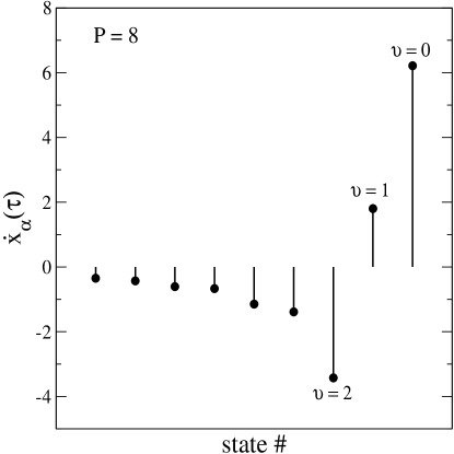
Figure 1: Level velocity spectrum associated with the states belonging to the polyad $P=8$ for the single $1:1$ resonant Hamiltonian.

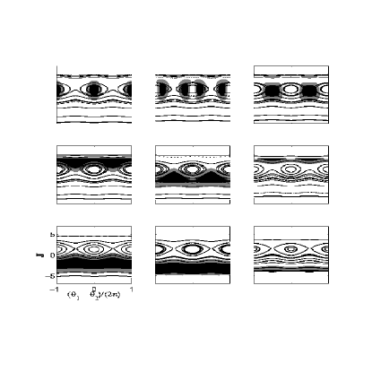
Figure 2: Husimi distributions associated with the states belonging to the polyad $P=8$ for the single $1:1$ resonant Hamiltonian. For comparison the Husimis are superimposed on the surface of sections. The top three panels show the resonant states with $\nu=0,1,2$.

In order to further check the correlation between level velocities and the phase space nature of the corresponding states the velocities and Husimis are computed for an integrable $2:1$ system $\widehat{H}=\widehat{H}_{0}+\tau\widehat{V}_{2:1}$ with the coupling strength $\tau=0.01$. The level velocities for the states belonging to the $2:1$ polyad $P=14$ are shown in Fig. (3). Again it is clear that the coupling is below the critical coupling and the level velocities show a characteristic pattern. The state $|14;0\rangle$ is expected to localize around the $2:1$ stable periodic orbit whereas the state $|14;3\rangle$ should be localized around the unstable periodic orbit. The husimis shown in Fig. (4) essentially confirm the expectations. In both the integrable cases, for coupling strengths near or above the critical value, the level velocities are large positive for the state in the center of the resonance island and equally large but negative for the seperatrix state. Thus the relative signs of the level velocities are crucial and provide information on the fixed points that dictate the phase space nature of the eigenstates. The absolute sign is clearly unimportant since a change in the sign of the coupling would interchange the signs of the velocities. In addition the state localized about the stable periodic orbit exhibits linear parametric motion and the velocity is closer to the classical value, computed using Eq. (27b), as compared to the state localized about the unstable periodic orbit.

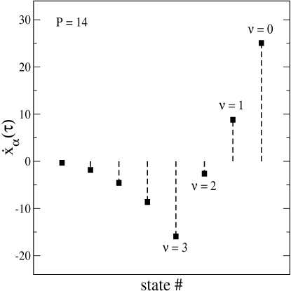
Figure 3: Level velocity spectrum associated with the states belonging to the polyad $P=14$ for the single $2:1$ resonant Hamiltonian.

The results of this section clearly indicate that the level velocities associated with the eigenstates are correlated to the structures in the classical phase space. In the following sections additional numerical examples are provided which highlight the correlation and the potential for using the level velocities to assign highly excited states of multiresonant Hamiltonians.

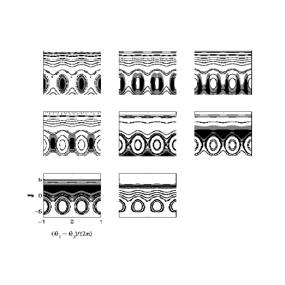
Figure 4: Husimi distributions associated with the states belonging to the polyad $P=14$ for the single $2:1$ resonant Hamiltonian. The top three and the middle left panels correspond to the resonant states with $\nu=0,1,2,3$ respectively.

III Application to nonintegrable systems

The states of single resonant Hamiltonians studied in the previous section can be assigned in various ways. Complications due to bifurcations can be sorted outkell ; annu with a detailed study of the classical-quantum correspondence for the system. However with the addition of another independent resonance the polyad constant of the motion is destroyed and assignments of the states becomes a nontrivial task. The underlying classical phase space can exhibit a rich variety of dynamics ranging from the near-integrable to the mixed to full chaos. An important observation that has emerged from the various studieswater ; ethy ; chbr ; dco ; annu ; jpc is that classical phase space structures can form the basis for a dynamical assignment of the various eigenstates of the system. The advantage of such a dynamical assignment is that it is based on invariant structures and directly reflects the relevant molecular motions in some energy range of interest. More importantly, such dynamical assignments are possible over the entire range of the phase space dynamics. For instance, a completely chaotic phase space at the outset seems to preclude any meaningful assignment of the states. Even for such hard chaotic systems it is wellknown that the eigenstates can be localized due to various quantum and classical effectsscar ; cantor1 ; cantor2 ; bsep ; diff . A prime example is the scarringscar of the eigenstates by the periodic orbits which has been studied in great detailscar2 over the years. In this case the relevant periodic orbits provide an avenue to dynamically assign the eigenstates.

From the perspective of studying IVR in isolated molecules a key observation is that the underlying phase space overwhelmingly belongs to the class of mixed dynamics. The fact that the effective spectroscopic Hamiltonians used to gain insights into IVR have the structure of a hierarchical local random matrixrev5 is largely responsible for the mixed nature of the phase space. Dynamical assignment of the highly excited eigenstates in such mixed phase space regimes is important and highly relevant. A significant bottleneck to such a classical-quantum correspondence based approach arises for systems with dimensionality greater than two. Any dynamical assignment of the eigenstates necessarily involves finding the important classical structures in the phase space and correlating them with the eigenstates or some phase space representation of the eigenstates. Already for a three degree of freedom system the Poincaré surface of sectionlicht is four dimensional and so is the computed Wigner or Husimi distribution of the eigenstates. This leads to diffculties in visually correlating the states with appropriate classical objects. One way to overcome this problem is to have algebraic measures and in this regard the results of the previous section suggest the level velocities as one possible candidate.

In order to assess the utility of the level velocities in providing a dynamical assignment of the eigenstates a model two resonance effective Hamiltonian $\widehat{H}=\widehat{H}_{0}+\tau_{11}\widehat{V}_{1:1}+\tau_{21}\widehat{V}_{2:1}$ is chosen. The parameters of the zeroth order Hamiltonian are as given in the previous section. The resonant coupling strengths are chosen to be $\tau_{11}=\tau_{21}=0.01$. The Hamiltonian is nonintegrable and the energy range $[8,9]$ is chosen as an example since the phase space exhibits mixed dynamics. The level velocities $\dot{x}_{\alpha}(\tau_{11})$ and $\dot{x}_{\alpha}(\tau_{21})$ are computed for some of the eigenstates in the selected energy range. Note that in the nonintegrable case the velocities can be expressed as:

$$\dot{x}_{\alpha}(\tau) = 2\sum_{P}\sum_{n_{1}=0}^{P}V_{nm}(n_{1};P)c^{*}_{n_{1}+m,\alpha}(\tau)c_{n_{1},\alpha}(\tau)$$ (15)

$$\equiv 2\sum_{P}\dot{x}_{\alpha}(\tau;P)$$ (16)

In this work the $\dot{x}_{\alpha}(\tau;P)$ will be called as the partial level velocities. The level velocities are scaled as

$$\widetilde{\dot{x}}_{\alpha}(\tau)=\frac{1}{\sigma_{E}}(\dot{x}_{\alpha}(\tau)-\langle\dot{x}_{\alpha}(\tau)\rangle)$$ (17)

where $\sigma_{E}$ is the variance of the velocities and $\langle\dot{x}_{\alpha}\rangle$ is the average of the level velocities. This is done since the velocities scale differently with the polyad $P$ and we would like to compare the two velocities for a given eigenstate. The scaled velocities are dimensionless, zero centered and have unit variance.

In Fig. (5) we show the scaled level velocity spectrum for selected eigenstates in the energy range $[8,9]$. In Table 1 the state energies, state IPRs in various basis, the scaled level velocities and the assignments are provided. The IPR of a state $|\alpha\rangle$ in a basis ${|b\rangle}$ can be obtained as

$$L_{b}(\alpha)=\sum_{b}|\langle b|\alpha\rangle|^{4}$$ (18)

In Table 1, $L_{0},L_{11}$, and $L_{21}$ denote the IPRs in the zeroth order number basis, the $1:1$ basis and the $2:1$ basis respectively. The standard interpretation of the IPR is that a low value signifies extensive mixing in the basis of choice whereas a high value indicates very little mixing of the basis states. The scaled velocity spectrum in Fig. (5) clearly shows different classes of states for which a brief description is provided below.

Table 1: Assignment of selected states for the nonintegrable system.

State	$E$	$L_{0}$	$L_{11}$	$L_{21}$	$\widetilde{\dot{x}}_{11}$	$\widetilde{\dot{x}}_{21}$	Assignment
68	8.038	0.35	0.39	0.89	-0.17	1.08	$P_{21}-1$
69	8.044	0.84	0.85	0.98	0.01	-0.79	$dl_{21}$
70	8.164	0.22	0.28	0.79	-0.30	-1.56	$u,P_{21}$
71	8.189	0.74	0.95	0.77	-0.65	-0.08	$dl_{11}$
72	8.203	0.99	1.00	0.99	-0.03	0.13	$l$
74	8.253	0.25	0.28	0.71	-0.53	-0.08	*
75	8.277	0.35	0.37	0.85	-0.05	2.58	$s,P_{21}-1$
77	8.313	0.21	0.75	0.26	-1.54	-0.38	$u,P_{11}$
79	8.338	0.94	0.99	0.95	-0.15	0.03	$l$
80	8.367	0.33	0.70	0.41	1.64	-0.46	$P_{11}$
82	8.423	0.99	1.00	0.99	-0.02	0.13	$l$
85	8.460	0.36	0.71	0.43	3.81	-0.38	$s,P_{11}$
86	8.473	0.21	0.23	0.81	0.11	1.07	$P_{21}$
88	8.514	0.38	0.39	0.93	0.08	-1.34	$u,P_{21}+1$
89	8.583	0.99	1.00	0.99	-0.01	0.13	$l$
91	8.650	0.83	0.97	0.85	-0.41	-0.08	$dl_{11}$
92	8.678	0.95	0.99	0.96	-0.11	0.03	$l$
93	8.682	0.22	0.25	0.76	-0.40	-0.27	*
94	8.683	0.99	1.00	0.99	-0.01	0.13	$l$
96	8.719	0.33	0.35	0.85	-0.05	2.89	$s,P_{21}$
98	8.763	0.48	0.47	0.96	-0.03	-1.33	$u,P_{21}+2$
99	8.848	0.24	0.58	0.27	-2.24	-0.38	$u,P_{11}+1$
100	8.869	0.18	0.20	0.27	-0.39	-0.17	*
101	8.898	0.18	0.19	0.53	0.35	0.84	*,$2:1$
102	8.958	0.96	0.99	0.97	-0.09	0.03	$l$
103	8.967	0.15	0.39	0.21	0.93	-0.83	*,$1:1,P_{11}+1$
104	8.972	0.37	0.40	0.51	0.24	-0.92	*,$2:1$

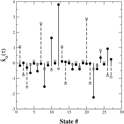
Figure 5: Scaled level velocity spectrum associated with the states in the energy range $[8,9]$ for the multiresonant Hamiltonian. The solid lines with filled circles correspond to the $1:1$ case and the dashed lines with open squares correspond to the $2:1$ case.

III.1 Local mode states

These states (72,79,82,89,92,94,102) are neither influenced by the $1:1$ perturbation nor the $2:1$ perturbation and hence nonresonant. The scaled velocities $\widetilde{\dot{x}}_{\alpha}(\tau_{11})$ and $\widetilde{\dot{x}}_{\alpha}(\tau_{21})$ are both very small indicating the local nature of these states. Note also that the IPRs are close to one in every basis for these set of states. As an example, the husimi of state 94 superimposed on the surface of section is shown in Fig. (6a). The zeroth order quantum numbers $(n_{1},n_{2})$ are good quantum numbers for the local mode states. In Table 1 such states are denoted by ’$l$’.

III.2 Distorted local mode states

As suggested by the name the distorted local mode states (69,71,91) are states that are lying close to either one of the resonance zones. Thus the husimi distribution of such states are distorted but topologically nonresonant. One such example is shown in Fig. (6b) for the state 71. The level velocities clearly indicate the particular resonance zone to which the states are in proximity. This is precisely the reason that the state 71 is labeled as ’$dl_{11}$’. The IPR values are also high and essentially agree with the assignments from the level velocity spectrum. The zeroth order quantum numbers are not so good a label for these distorted states. It is also possible to think of these states as a kind of ’borderline’ states and hence a slight increase in the appropriate resonance coupling strength will render them resonant.

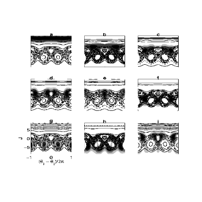
Figure 6: Husimis for selected states superimposed on the corresponding surface of sections. See the text for details.

III.3 Resonant states

The resonant states (68,70,75,77,80,85,86,88,96,98,99) show up in the velocity spectrum in Fig. (5) as states with large positive or negative velocities. In accordance with our discussions in the previous sections these states are localized in one or the other resonance zone. Moreover states with large positive velocity are expected to be localized about the corresponding stable periodic orbit. On the other hand states with large negative velocities are expected to be localized about the corresponding seperatrix region. For example state 85 has a large positive $\widetilde{\dot{x}}_{\alpha}(\tau_{11})$ and comparitively negligible $\widetilde{\dot{x}}_{\alpha}(\tau_{21})$. Consequently this state is anticipated to be localized exclusively in the $1:1$ resonance zone and the Husimi distribution to be localized about the $1:1$ resonance island in the underlying phase space. That this is indeed the case is confirmed in Fig. (6e). Thus state 85 is labeled by ’$s$’ indicating localization about the stable periodic orbit. In Table 1 we have also appended a label $P_{11}$ suggesting that the particular $1:1$ polyad $P_{11}$ is almost a good quantum number to assign the state. Similarly state 96 is localized about the $2:1$ island according to the level velocities and Fig. (6g) supports the assignment. An approximate polyad $P_{21}$ is also attached to this state.

In order to complete the assignment the approximate polyads $P_{11}$ and $P_{21}$ need to be determined. To this end it is useful to examine the partial level velocities $\dot{x}_{\alpha}(\tau;P)$ as a function of $P$ for the corresponding states. $P$ is chosen appropriately for the particular resonance. Thus, $P=n_{1}+n_{2}$ for the $1:1$ resonance and $P=2n_{1}+n_{2}$ for the $2:1$ resonance. It is important to note that this information is obtained enroute to computing the level velocity of a state and does not require a seperate computation. In Fig. (7e,g) the partial velocities are shown for states 85 and 96 respectively. It is clear from the figure that $P_{11}=10$ and $P_{21}=14$. A similar analysis can be done on all the states and as an example the partial velocities are shown in Fig. (7a) for the state 94. One can immediately assign this local mode state as $(n_{1},n_{2})=(0,15)$

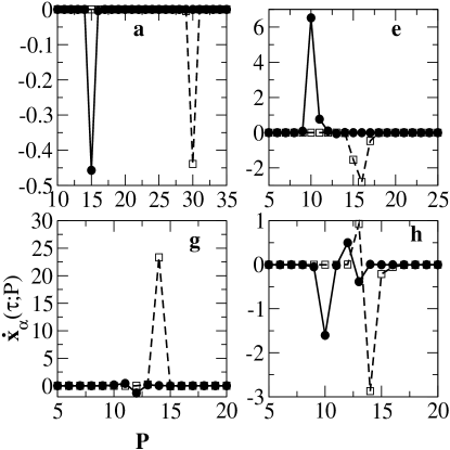
Figure 7: Unscaled partial level velocities for selected states as a function of the polyad. The labeling of the figures corresponds to that in Fig. (6). The solid lines with filled circles correspond to the $1:1$ case ($P=n_{1}+n_{2}$) and the dashed lines with open squares correspond to the $2:1$ case ($P=2n_{1}+n_{2}$).

Once the resonant states with large positive velocities have been assigned the rest of the resonant states can be easily assigned as shown in Table 1. Two important properties of the level velocities guide the assignments. The first property is that for positive coupling constants the states localized about the stable periodic orbits with some approximate polyad $P$ are energetically higher than the states localized about the unstable periodic orbits belonging to $P$. Exceptions can occur due to bifurcations and this is discussed in the following section. Secondly, velocity of states with some approximate $P$ scale differently with $P$ for the $1:1$ and the $2:1$ resonances. Thus states belonging to the $2:1$ resonance are seperated more as compared to the states belonging to the $1:1$ resonance. A Chirikovchiri like estimate is also an indicator of the number of states bound by the resonance. Moreover, studying the partial velocities helps in confirming the assignments. In Figs. (6c,f) we show the Husimi distributions for the states 77 and 70 respectively. The Husimis are localized in the chaotic regions corresponding to the integrable limit seperatricies and lend support to the assignments in Table 1 where the label ’$u$’ is used to denote such states.

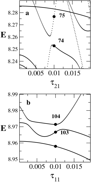
Figure 8: (a) Sharp avoided crossing between states 74 and 75 as a function of the $2:1$ coupling parameter $\tau_{21}$. (b) Broad avoided crossing between states 103 and 104 as a function of the $1:1$ coupling parameter $\tau_{11}$. States are analysed in this work for $\tau_{11}=\tau_{21}=0.01$.

III.4 Mixed states

There are a few states (74,93,100,103) which cannot be assigned in a straightforward fashion. As an example state 74 according to the IPR values should be predominantly a $2:1$ resonant state. However the level velocities show the opposite trend. In Fig. (6h) we show the Husimi for state 74 superimposed on the surface of section. It is clear that the state is delocalized over both the chaotic as well as the regular regions of the phase space as compared to the other states in Fig. (6). The Husimi, however, is peaked in the $2:1$ regions of the phase space in agreement with the IPR values. These observations are symptomatic of avoided crossings since at an avoided crossing regular and chaotic states can mix. Indeed on examining the variation of the eigenvalues with the $2:1$ coupling parameter $\tau_{21}$, shown in Fig. (8a), it is seen that the state 74 is involved in an avoided crossing with the regular state 75. The important observation is that the state 74 is located close to the center of the avoided crossing. This explains the low value for the velocity $\widetilde{\dot{x}}_{\alpha}(\tau_{21})$ and the apparent difficulty in the assignment of the state 74. The partial velocities for the state 74 shown in Fig. (7h) clearly demonstrate the delocalized nature of the state. The assignment of the state 93 is complicated due to similar reasons. The states 100 and 101 are also close to being involved in an avoided crossing. In this case the velocities can be used to provide a nominal assignment.

On the other hand states 103 and 104 are again close to being involved in an avoided crossing as shown in Fig. (8b). Note that the parameter being varied in Fig. (8b) is the $1:1$ coupling strength $\tau_{11}$. The husimi distribution for the state 103 is shown in Fig. (6i) and looks topologically very much like the case in Fig. (6d) except for the peak in the $2:1$ region. Again the level velocities can be used to nominally assign the state 103 as a $1:1$ state belonging to the polyad $P_{11}+1$. Thus the mixed states arising in this energy range are primarily due to two state avoided crossings.

IV Discussion and summary

The main focus of the present work is to come up with techniques which would allow a dynamical assignment of highly excited states of multiresonant, multidimensional ($>2$) Hamiltonians. It is well known that an intimate knowledge of the various classical phase space structures is the first important step towards such dynamical assignments. However obtaining a detailed picture, akin to the two dimensional systems, of the phase space structure for systems with three or larger degrees of freedom is diffcult. In this paper we have argued that the phase space nature of an eigenstate is encoded in the manner that it responds to variation of specific parameters of the Hamiltonian. In other words, the level velocity associated with an eigenstate is strongly correlated to the phase space nature of the eigenstate. Theoretical arguments for the observed correlation have been provided for single resonant systems. In a way the current work begins to provide a basis for understanding and utilizing the usual energy correlation diagrams. We have shown the utility of the level velocities in a dynamical assignment of the highly excited states of a 2-mode multiresonant Hamiltonian. It is important to point out here that our approach does not require explicit determination of the periodic orbits for the system. It is equally relevant to mention that the level velocity approach is independent of the dimensionality of the system and is manifestly basis invariant. Thus the current work is a first step in coming up with algebraic measures facilitating the study of the classical-quantum correspondence for multidimensional systems.

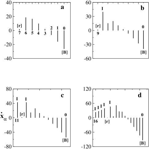
Figure 9: Level velocity spectra for the HCP molecule for the various CP stretch-bend polyads $P$. $[r]$ and $[B]$ are stable periodic orbits. (a) $P=14$ (b) $P=18$. Notice the perturbation of the positive part of the level velocities. $I$ labels the isomerization state. (c) $P=22$ (d) $P=32$.

The method proposed in this paper for the dynamical assignment of highly excited states, however, has a few weakpoints. Firstly, it is quite possible for the level velocity of a particular eigenstate to be close to zero. For example, for coupling strengths near the critical value, the $1:1$ state $|6;3\rangle$ will exhibit zero velocity. Assigning such states solely on the basis of level velocities will be problematic. Secondly, as demonstrated in the last section, states involved in an avoided crossing can pose problems for the assignment as well. This is not surprising since such states are difficult to assign by any of the existing methods. Nevertheless, taking linear combinations of the two states and assigning the demixed states is one possible solution. In both instances it is still possible to gain insights into the states by examining other measures like the IPRs in conjunction with the level velocities.

One of the important issues that we have not addressed has to do with the effect of the various bifurcationskell ; annu ; jpc on the level velocity spectrum. In this work we have explicitly shown the important role played by the fixed points in the classical phase space as far as the level velocities are concerned. Bifurcationslicht ; weyl are associated with creation or destruction of fixed points and hence signal qualitative change in the dynamics. Thus, it is clear that the level velocities would be quite sensitive to bifurcations. Work is in progress in our group to study the fingerprints of bifurcations on the level velocity spectrum in a sytematic fashion. However, we conclude this paper by showing some preliminary work on the HCP molecule in order to gauge the utility of the level velocities. We have chosen HCP as an example due to the fact that the system has been investigated experimentallyhcpexpt and thoroughly studied from the classical-quantum perspectiveannu ; jpc . The effective spectroscopic Hamiltonianhcp2000 for HCP involves a $1:2$ Fermi resonant coupling between the bend and the CP stretch. Thus there exists a polyadnote $P=v_{2}+2v_{3}$ with $v_{2}$ and $v_{3}$ refering to the bend and the CP stretch modes respectively. The states can be assigned in terms of the vibrational angular momentum, the number of quanta in the CH stretch $(v_{1})$, and the polyad $P$. Further for every given $P$ there are $P/2+1$ levels indexed by $i=0$ at the top of the polyad and $i=P/2$ at the bottom of the polyad. It has been establishedhcp2000 that for $v_{1}=0$ and up to $P=14$ the states evolve smoothly from being pure CP stretch at the bottom of the polyads to being approximately pure bend at the top of the polyads. However starting at $P=18$ a new family of states, called isomerization states, come into existence due to a saddle node bifurcation of the periodic orbits. Above $P=22$ the isomerization states are almost pure bend and closely follow the minimum energy path leading from HCP to CPHannu . Keeping this information in mind in Fig. (9) we show the unscaled level velocity spectrum corresponding to polyads $P=14,18,22$, and $32$ for the HCP molecule. It is crucial to note that for the effective spectroscopic Hamiltonian fit the Fermi resonant coupling is negativehcp2000 . We thus anticipate a large negative velocity for the state localized around the stable periodic orbit. It is also known that for low polyad values there are two stable periodic orbits denoted by $[r]$ and $[B]$. The velocity spectrum for $P=14$ shown in Fig. (9a) clearly indicates that the $i=0$ state is localized around the $[B]$ periodic orbit. From our theoretical analysis and the appendix we expect the state associated with the $[r]$ periodic orbit to have a very small velocity which is confirmed in Fig. (9a) for state $i=7$. The velocity spectrum suggests that most of the states are resonant and indeed the classical estimate $(-28.51)$ (cf. Eq. (27b)) for the velocity of the state $i=0$ is very close to the computed value $(-26.36)$. In Fig. (9b) the velocity spectrum is shown for $P=18$. For this case we clearly see a pertubation in the spectrum in the positive velocity region and the resulting isomerization state is labeled as $I$. The negative velocity region is unperturbed. The perturbation is quite prominent in Figs. (9c,d) corresponding to the $P=22$ and the $P=32$ cases. In every case the velocity of the $[B]$ state is close to the classical estimate. Given that the negative portion of the velocity spectrum is unperturbed we conclude that the bifurcation is creating a stable periodic orbit $(SN)$ and an unstable periodic orbit $(\overline{SN})$ at $\psi=\pi/2$ in the reduced phase space. Thus the isomerization states form a sequence from being localized about the $SN$ periodic orbit to the $\overline{SN}$ periodic orbit. In this instance as the saddle node bifurcation creates the stable/unstable pair at the same angle $\psi=\pi/2$ the level velocities for states localized about both the periodic orbits are expected to be large positive. The caricature of the phase space just described agrees well with the earlier studieshcp2000 ; jpc . It is clear that the level velocity spectrum is correlated with the phase space structure and capable of detecting nontrivial changes in the phase space due to the bifurcations.

This work is a first step towards developing tools suitable for studying classical-quantum correspondence in multidimensional systems. The systems studied in this paper are certainly encouraging and warrant further study of the level velocities and different measures based on the level velocities. One such sensitive measure has been proposed recentlykct which correlates the level velocities with the eigenstate resolved spectrum of the molecule in order to gain insights into the IVR process. Currently we are exploring the utility of the level velocities in assigning the states of three degree of freedom multiresonant Hamiltonians which are effectively two dimensional due to the existence of a superpolyad number. Spectroscopic Hamiltonians have been determined for many such effectively two dimensional systems like H₂Obagg , CHBrClFbeil , and DCOtemp . Preliminary studiesprelim on such systems indicate that the level velocity spectrum is well suited for the purpose of dynamical assignment of the eigenstates. Studies are also underway of true three degree of freedom systems in order to test the approach and for insights into the highly excited states of such systems from the classical- quantum correspondence perspectives.

V Acknowledgements

SK gratefully acknowledges the Department of Science and Technology and the Council for Scientific and Industrial Research, India for financial support.

Appendix: Classical insight into the level velocities

In this appendix we provide a classical argument for the scaling of the level velocities with the polyad $P$ for a general single resonance Hamiltonian.

The $n:m$ resonant Hamiltonian corresponding to the classical limit of the quantum Hamiltonian is:

$$H({\bf I},{\bm{\theta}})=H_{0}({\bf I})+2\tau I_{1}^{m/2}I_{2}^{n/2}\cos(m\theta_{1}-n\theta_{2})$$ (19)

The classical limit Hamiltonian can be reduced to an effective one dimensional one by using the following generating function

$$F_{2}=I\left(\theta_{1}-\frac{n}{m}\theta_{2}\right)+P_{c}\theta_{2}$$ (20)

The reduced Hamiltonian is obtained as

$$H(I,\phi;P_{c})=H_{0}(I;P_{c})+2\tau V(I;P_{c})\cos m\phi$$ (21)

with

$$V(I;P_{c})=I^{m/2}\left(P_{c}-\frac{n}{m}I\right)^{n/2}$$ (22)

The action $P_{c}$ is a constant of the motion since the Hamiltonian is ignorable in the angle conjugate to $P_{c}$. $P_{c}=n/mI_{1}+I_{2}$ is the classical analog of the polyad number.

The fixed points in the $(I,\phi)$ plane correspond to periodic orbits in the full phase space. Using $\dot{I}=0=\dot{\phi}$ we obtain the fixed points as $\bar{\phi}=0,\pm\pi/m$. The solution $\bar{I}=0$ is discarded since it is unphysical and the other root of $\bar{I}$ is of no interest here since that corresponds to all the excitation in the first mode. Using the value of the angle $\phi$ at the fixed points the corresponding actions are obtained by a solution to the algebraic equation:

$$\frac{\partial H_{0}}{\partial I}\pm 2\tau g(I;P_{c})=0$$ (23)

where

$$g(I;P_{c})=\frac{dV(I;P_{c})}{dI}$$ (24)

This nonlinear equation is solved numerically to obtain the periodic orbits of the system.

In this appendix, however, attention is focused on the analysis of the function

$$v(I,\phi;P_{c})=\frac{\partial H}{\partial\tau}=2V(I;P_{c})\cos m\phi$$ (25)

which occurs in the semiclassical approximation Eq. (14) for the quantum level velocities. Interest in this function arises from exploring the maximum and minimum values that this function can take at the fixed points in the $(I,\phi)$ space. Inspecting the $I$ and $\phi$ derivative of $v(I,\phi;P_{c})$

$$\frac{\partial}{\partial\phi}v(I,\phi;P_{c}) = -2mV(I;P_{c})\sin m\phi$$ (26a)

$$\frac{\partial}{\partial I}v(I,\phi;P_{c}) = 2g(I;P_{c})\cos m\phi$$ (26b)

it is clear that the critical points in the $\phi$ variable are identical with those of the fixed points. The critical points arising from the $I$ variable are $\bar{I}=0,(m/n)P_{c},m^{2}P_{c}/n(m+n)$. Note that demanding $g(I;P_{c})=0$ is tantamount to being on the center of the resonance line and hence the stable periodic orbit. The first two critical values give rise to zero velocities and correspond to the “edge” states in a given polyad multiplet. The third critical point gives rise to the velocities:

$$v(\bar{I}^{(3)},0;P_{c}) = -v(\bar{I}^{(3)},\pi/m;P_{c})$$ (27a)

$$= 2\left[\frac{\mu^{n-m}}{(1+\mu)^{n+m}}\right]^{1/2}P_{c}^{(m+n)/2}$$ (27b)

where, $\mu=n/m$. From the above one immediately sees that the classical object takes the same absolute value at the stable and unstable fixed points. Moreover, the classical analog exhibits the identical scaling with the polyad $P_{c}$ as seen in exact quantum studies done previously. In fact it is seen in the quantum studies that the resonant eigenstate $|P;\nu\rangle$ with $\nu=0$ i.e., state localized on the stable fixed point shows very good agreement with the above classical estimate.

References

- (1) C. E. Hamilton, J. L. Kinsey, and R. W. Field, Annu. Rev. Phys. Chem. 37, 493 (1986).
- (2) K. K. Lehmann, G. Scoles, and B. H. Pate, Annu. Rev. Phys. Chem. 45, 241 (1994).
- (3) D. J. Nesbitt and R. W. Field, J. Phys. Chem. 100, 12735 (1996).
- (4) G. S. Ezra, Adv. Class. Traj. Meth. 3, 35 (1998).
- (5) M. Gruebele, Adv. Chem. Phys. 114, 193 (2000).
- (6) J. C. Keske and B. H. Pate, Annu. Rev. Phys. Chem. 51, 323 (2000).
- (7) M. J. Davis, Int. Rev. Phys. Chem. 14, 15 (1995).
- (8) T. Uzer, Phys. Rep. 199, 73 (1991).
- (9) E. J. Heller, J. Phys. Chem. 99, 2625 (1995).
- (10) S. Keshavamurthy and G. S. Ezra, J. Chem. Phys. 107, 156 (1997).
- (11) Z. Lu and M. E. Kellman, J. Chem. Phys. 107, 1 (1997).
- (12) M. P. Jacobson, C. Jung, H. S. Taylor, and R. W. Field, J. Chem. Phys. 111, 600 (1999).
- (13) C. Jung, E. Ziemniak, and H. S. Taylor, J. Chem. Phys. 115, 2499 (2001).
- (14) C. Jung, H. S. Taylor, and E. Atilgan, J. Phys. Chem. A, to appear (2002).
- (15) H. Ishikawa, R. W. Field, S. C. Farantos, M. Joyeux, J. Koput, C. Beck, and R. Schinke, Annu. Rev. Phys. Chem. 50, 443 (1999).
- (16) M. Joyeux, S. C. Farantos, and R. Schinke, J. Phys. Chem. A, to appear (2002).
- (17) See M. E. Kellman, Annu. Rev. Phys. Chem. 46, 395 (1995) and references therein.
- (18) S. C. Farantos, Int. Rev. Phys. Chem. 15, 345 (1996).
- (19) V. I. Arnold, Dokl. Nauk. Akad. SSSR 156, 9 (1964).
- (20) See for example, M. Olle and D. Pfenniger in Hamiltonian Systems with Three or More Degrees of Freedom, Ed. C. Simó, NATO-ASI 533, 518 (1999).
- (21) K. Husimi, Proc. Phys. Math. Soc. Jpn. 22, 264 (1940).
- (22) E. P. Wigner, Phys. Rev. 40, 749 (1932).
- (23) Hamiltonian Systems with Three or More Degrees of Freedom, Ed. C. Simó, NATO-ASI 533, 1999.
- (24) A. J. Lichtenberg and M. A. Lieberman, Regular and Chaotic Dynamics, Springer-Verlag, Second edition, chapter 6, 1992.
- (25) C. C. Martens, J. Stat. Phys. 68, 207 (1992).
- (26) C. C. Martens, M. J. Davis, and G. S. Ezra, Chem. Phys. Lett. 142, 519 (1987).
- (27) J. Laskar, Physica D 67, 257 (1993).
- (28) D. J. Thouless, Phys. Rep. 13, 93 (1974).
- (29) K. M. Atkins and D. E. Logan, Phys. Lett. A 162, 255 (1992).
- (30) D. M. Leitner and P. G. Wolynes, Chem. Phys. Lett. 258, 18 (1996).
- (31) S. A. Schofield, R. E. Wyatt, and P. G. Wolynes, J. Chem. Phys. 105, 940 (1996).
- (32) M. P. Jacobson and R. W. Field, Chem. Phys. Lett. 320, 553 (2000).
- (33) E. J. Heller, E. B. Stechel, and M. J. Davis, J. Chem. Phys. 73, 4720 (1980).
- (34) J. Svitak, Z. Li, J. Rose, and M. E. Kellman, J. Chem. Phys. 102, 4340 (1995).
- (35) D. W. Noid, M. L. Koszykowski, M. Tabor, and R. A. Marcus, J. Chem. Phys. 72, 6168 (1980).
- (36) B. Ramachandran and K. G. Kay, J. Chem. Phys. 99, 3659 (1993).
- (37) S. Keshavamurthy, J. Phys. Chem. 105 A, 2668 (2001) and references therein.
- (38) P. Pechukas, Phys. Rev. Lett. 51, 943 (1983).
- (39) K. Nakamura and M. Lakshmanan, Phys. Rev. Lett. 57, 1661 (1986).
- (40) See F. Haake, Quantum Signatures of Chaos, Springer-Verlag, Second ed., 2000.
- (41) B. D. Simons and B. L. Altshuler, Phys. Rev. B 48, 5422 (1993).
- (42) P. Gaspard, S. A. Rice, H. J. Mikeska, and K. Nakamura, Phys. Rev. 42 A, 4015 (1990).
- (43) Y. V. Fyodorov and A. D. Mirlin, Phys. Rev. B 51, 13403 (1995).
- (44) T. Takami and H. Hasegawa, Phys. Rev. Lett. 68, 419 (1992).
- (45) N. R. Cerruti, A. Lakshminarayan, J. H. Lefebvre, and S. Tomsovic, Phys. Rev. E 63, 016208 (2001).
- (46) A. Lakshminarayan, N. R. Cerruti, and S. Tomsovic, Phys. Rev. E 63, 016209 (2001).
- (47) S. Keshavamurthy, N. R. Cerruti, and S. Tomsovic, J. Chem. Phys. (to appear, 2002).
- (48) L. E. Fried, G. S. Ezra, J. Chem. Phys. 86, 6270 (1987).
- (49) H. Dübal and M. Quack, J. Chem. Phys. 81, 3779 (1984).
- (50) Y. Weissman and J. Jortner, J. Chem. Phys. 77, 1486 (1982).
- (51) See for example, A. M. Ozorio de Almeida, Hamiltonian Systems: Chaos and Quantization, Cambridge University Press, Cambridge, 1988.
- (52) A. M. Ozorio de Almeida, Phys. Rep. 295, 265 (1998) and references therein.
- (53) R. G. Littlejohn, unpublished lecture notes.
- (54) M. V. Berry, Phil. Trans. Roy. Soc. Lon. 287, 237 (1977).
- (55) S. Keshavamurthy, unpublished notes.
- (56) J. B. Delos, R. L. Waterland, and M. L. Du, Phys. Rev. A 37, 1185 (1988).
- (57) K. Takahashi, J. Phys. Soc. Jpn. 55, 762 (1986).
- (58) E. J. Heller, Phys. Rev. Lett. 53, 1515 (1984).
- (59) See L. Kaplan and E. J. Heller, Ann. Phys. 264, 171 (1998) and references therein.
- (60) R. Ketzmerick, G. Petschel, and T. Geisel, Phys. Rev. Lett. 69, 695 (1992).
- (61) G. Radons, T. Geisel, and J. Rubner, Adv. Chem. Phys. LXXIII, 891 (1989).
- (62) O. Bohigas, S. Tomsovic, and D. Ullmo, Phys. Rep. 223, 43 (1993).
- (63) S. Fishman, D. R. Grempel, and R. E. Prange, Phys. Rev. A 36, 289 (1987).
- (64) B. V. Chirikov, Phys. Rep. 52, 263 (1979).
- (65) H. Ishikawa, C. Nagao, N. Mikami, and R. W. Field, J. Chem. Phys. 109, 492 (1998).
- (66) M. Joyeux, D. Sugny, V. Tyng, M. E. Kellman, H. Ishikawa, R. W. Field, C. Beck, and R. Schinke, J. Chem. Phys. 112, 4162 (2000).
- (67) In the interests of easy comparison with the earlier work on HCP we have used the same conventions and notations as in Ref. hcp2000, .
- (68) J. E. Baggot, Mol. Phys. 65, 739 (1988).
- (69) A. Beil, D. Luckhaus, and M. Quack, Ber. Bunsenges. Phys. Chem. 100, 1853 (1996).
- (70) A. Troellsch and F. Temps, Z. Phys. Chem. 215, 207 (2001).
- (71) A. Semparithi and S. Keshavamurthy, to be submitted.