Studies with Ultracold Metastable Hydrogen

Abstract

This thesis describes the first detailed studies of trapped metastable ($2S$-state) H. Recent apparatus enhancements in the MIT Ultracold Hydrogen group have enabled the production of clouds of at least $5\times 10^{7}$ magnetically trapped $2S$ atoms at densities exceeding $4\times 10^{10}$ cm^-3 and temperatures below 100 $\mu$K. At these densities and temperatures, two-body inelastic collisions between $2S$ atoms are evident. From decay measurements of the $2S$ clouds, experimental values for the total two-body loss rate $K_{2}$ are derived: $K_{2}=1.8^{+1.8}_{-0.7}\times 10^{-9}$ cm³/s at 87 $\mu$K, and $K_{2}=1.0^{+0.9}_{-0.5}\times 10^{-9}$ cm³/s at 230 $\mu$K. These values are in range of recent theoretical calculations for the total $2S$-$2S$ inelastic rate constant. Experimental upper limits for $K_{12}$, the rate constant for loss due to inelastic $1S$-$2S$ collisions, are also determined. As part of the discussion and analysis, results from numerical simulations to elucidate $2S$ spatial distributions, evolution of the $2S$ cloud shape, and fluorescence behavior in the magnetic trap are presented. This work serves as a bridge to future spectroscopy of trapped metastable H with the potential to test quantum electrodynamics (QED) and improve fundamental constants.

To my mom and dad

Chapter 0 Introduction

The $2S$ state of hydrogen is metastable because it decays by two-photon spontaneous emission. It has a natural lifetime of 122 ms. This is not the only sense in which this species is long-lived, however. It has enjoyed a long and fruitful life in atomic physics research. From the explanation of the Balmer series of spectral lines, to the groundbreaking first calculation of a two-photon decay rate, on through numerous rf and optical measurements of the Lamb shift, metastable hydrogen has played a key role. The studies described in this thesis are part of a new chapter in this unfolding history, one which will likely lead to further insight into fundamental physics.

Traditionally, metastable H has been studied in discharge cells or in atomic H beams which have been excited by a laser or by electron bombardment. In the MIT Ultracold Hydrogen Group, the application of a high-power, narrow-linewidth UV laser system to magnetically trapped $1S$-state hydrogen has produced clouds of metastables at temperatures ranging from 300 mK down to 20 $\mu$K. Recent improvements to the apparatus at MIT have allowed generation of clouds of more than $10^{7}$ $2S$ atoms at densities greater than $10^{10}$ cm^-3 and lifetimes of nearly 100 ms. These trapped metastable clouds are promising new samples for collisional physics and precision spectroscopy.

In the first section of this introduction, the impetus for studying cold, trapped metastable H is futher discussed. This is followed by a brief overview of concepts relevant to magnetic trapping and $1S$-$2S$ excitation.

1 Motivations

1 Metastable H Collisions

A cold gas of metastable H is an interesting laboratory for collisional physics. One reason for this is that a $2S$ atom carries more than 10 eV of internal energy, enough to cause ionization in many targets and to drive chemical reactions. When metastables collide with one another, the possible outcomes include Penning ionization, the formation of molecular ions, excitation transfer to short-lived $2P$ states, and transitions between hyperfine states. If the $2S$ atoms are excited from a background $1S$ gas, then several $1S$-$2S$ collision processes can occur as well. Various aspects of cold, elastic $1S$-$2S$ interactions have already been investigated by our group [1, 2] and by several theory collaborations [3, 4, 5].

Collisions between metastables have previously been studied at high effective temperatures ($T>48$ K) [6], where the total inelastic rate constant is several orders of magnitude larger than at $T=0$ [7, 8]. At high temperatures, the rate constant for excitation transfer or “collisional quenching” has been predicted to limit the lifetime of a metastable gas to about 40 $\mu$s at a density of 10¹⁰ cm^-3[9]. With cold, magnetically trapped clouds of $2S$ atoms, the lifetime at this density is found to be tens of milliseconds. By observing the decay behavior of a metastable cloud, we can learn about $2S$-$2S$ and $1S$-$2S$ inelastic collisions. This thesis presents the first measurements of the total $2S$-$2S$ inelastic collision rate at low temperatures. These measurements extend into the theoretically predicted “ultracold” regime, where both elastic and inelastic collisions are parametrized by a single constant, the complex scattering length [7, 10].

2 Spectroscopy of Metastable H

Although the collisional physics of metastables is worth studying for its own sake, a deeper understanding of these interactions also helps set the stage for ultraprecise spectroscopy of metastable H. The absolute frequencies of transitions from the $2S$ to higher-lying states of H can be combined with the $1S$-$2S$ interval, currently the most accurately known of all optical transition frequencies, to simultaneously determine the $1S$ Lamb shift and the Rydberg constant [11, 12]. The former quantity is predominantly comprised of quantum electrodynamics (QED) corrections to the Dirac solution for the hydrogen atom, and it has been called the most sensitive test of QED in an atom. The Rydberg constant, $R_{\infty}=m_{e}c\alpha^{2}/2h$, is already the most accurately known of all fundamental constants. It provides a link between the electron mass, the speed of light, the fine structure constant, and Planck’s constant. Thus, spectroscopy of metastable H provides a way to not only test the state-of-the-art of QED theory but also improve the accuracy of fundamental constants [12, 13, 14].

Several $2S$-$nS/D$ frequency intervals, where $n>3$, have been measured with impressive accuracy by F. Biraben and collaborators using Doppler-free two-photon spectroscopy [15, 16, 17, 12]. Currently, the best experimental values for both the Lamb shift and Rydberg constant are limited by uncertainty in $2S$-$nS/D$ frequencies [12]. The Biraben experiments were conducted with atomic beams in which the interaction time of metastables with a laser was limited to a few hundred microseconds. To achieve an efficient excitation rate required laser intensities of several kilowatts per square centimeter. The resulting AC Stark shifts were the primary source of uncertainty in the measurement. With a cold, trapped sample of metastable H, the interaction times between the excitation laser and the atoms can be much larger, and laser intensities can be much lower. Another source of systematic error in the beam experiments was the quadratic DC Stark shift of higher-lying $D$ states. Since excitation rates can be much higher in a trapped sample, one can afford to concentrate on weaker $2S$-$nS$ transitions, which are less sensitive to stray electric fields.

Once an excitation laser is tuned to a two-photon $2S$-$nS$ resonance, its absolute frequency can be calibrated directly against the primary cesium standard or against the $1S$-$2S$ frequency, which is now a de facto optical frequency standard [13]. The frequency metrology can be accomplished with a mode-locked femtosecond laser which produces a broad, coherent frequency comb [18, 19, 20]. Frequency measurements made in this way using ultracold hydrogen will potentially allow an order of magnitude improvement in both the Lamb shift and Rydberg constant [21].

Since many transitions originating in the $2S$ state are accessible with diodes and other readily available lasers, trapped metastable H as a spectroscopic sample opens the door to other interesting studies as well. These include photoassociation experiments and measurements of cold collision parameters involving higher-lying states of H.

3 Quantum Atom Optics

Due to its large internal energy, cold metastable H is interesting for “quantum atom optics” experiments involving single-atom detection. The possibilities include measurements to probe atom-atom correlations [22], atom interferometry, and atom holography [23]. A metastable H atom is readily detected in an ionizing collision on an electron-multiplying detector. Alternatively, one can detect the Lyman-$\alpha$ photon emitted after quenching at a surface or by a localized electric field. To detect individual metastables generated from ultracold hydrogen, they must be coupled out of the magnetic trap. This can be accomplished by inducing an appropriate rf or optical transition to an untrapped atomic state or by simply turning off the magnetic trap. Several single-atom detection experiments involving cold, metastable noble gases have already been demonstrated [22, 23] or are in progress [24]. It may also be possible to generate a highly directional metastable H beam from an ultracold sample using photon recoil in a Raman transition [25] or in the initial $1S$-$2S$ excitation (see Sec. 3). A bright beam of cold metastables may be ideal for atom lithography [26, 27].

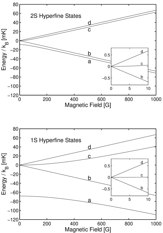
Figure 1: Comparison of hyperfine-Zeeman diagrams for the $1S$ and $2S$ manifolds of H. For each case, energy is referenced to the $F=1$ vertex, where the $b$, $c$, and $d$ states are degenerate. The larger plots show all four hyperfine states over the magnetic field range relevant during forced evaporation of magnetically trapped H. In the inset plots, the $b$, $c$, and $d$ states are shown for the 0-10 G range of magnetic fields typically experienced by samples at 100 $\mu$K.

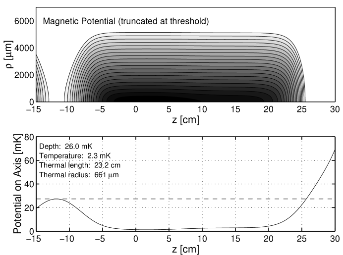
Figure 2: Magnetic potential as a function of cylindrical coordinates $\rho$ and $z$ for a standard trap configuration (Trap Z of Ch. 3). The potential has been calculated numerically from the known magnet geometry and currents. In the upper half of the figure, the region of magnetic potential below the trap threshold is depicted by a shaded contour plot; the shading is darkest at the trap minimum. The lower half of the figure shows the magnetic profile along the trap axis. The magnetic saddlepoint, which defines the trap threshold (dashed line), is located near $z=-12$ cm. Dimensions are given for the $1S$ cloud at the temperature experimentally achieved in this trap. Similar figures will be used in this thesis to describe the shape and characteristics of other samples. The coordinate system origin follows a convention of the MIT Ultracold Hydrogen Group.

2 Hyperfine States and Magnetic Trapping

The hyperfine state energies for both the $1S$ and $2S$ levels of H are plotted as a function of magnetic field in Fig. 1. The hyperfine interaction energy, which scales as $1/n^{3}$ for $S$ states, is only $1/8$ as large for metastable hydrogen as for the ground state. Except for this hyperfine energy scaling, the $2S$ manifold is basically identical to the $1S$ manifold.

In both levels, the hyperfine states are conventionally labeled $a$, $b$, $c$, and $d$, in order of increasing energy. At low magnetic field, these states correspond to the total angular momentum states $(F=0,m_{F}=0)$, $(F=1,m_{F}=-1)$, $(F=1,m_{F}=0)$, and $(F=1,m_{F}=1)$, respectively. In an inhomogeneous magnetic field, the “low-field seeking” $c$ and $d$ states can be trapped around a minimum of the magnetic field [28, 29]. Since $c$-state atoms rapidly undergo spin-exchange collisions and transition to other hyperfine states, the sample which collects in a magnetic trap ultimately contains only $d$-state atoms. The trap loading process for $1S$ atoms will be discussed extensively in Sec. 4.

Trapped metastable hydrogen is produced by two-photon excitation of trapped $(1S,d)$ atoms [30]. The two-photon selection rules are $\Delta F=0$ and $\Delta m_{F}=0$; thus, only trapped $(2S,d)$ atoms are excited. Furthermore, since the magnetic potential energy of both $(1S,d)$ and $(2S,d)$ atoms is to an excellent approximation

$$U=\mu_{B}B,$$ (1)

where $\mu_{B}$ is the Bohr magneton and $B$ the local magnetic field strength, the trapping potentials experienced by both species is the same.

The trap in our apparatus is of the Ioffe-Pritchard variety [32]. To a good approximation, the magnetic field has cylindrical symmetry about an axis known as the “trap axis.” With an aspect ratio typically between 150:1 and 400:1, the axial dimension of the trap is much longer than the radial dimension. A typical field geometry is depicted in Fig. 2. The depth of the trap is determined by a saddlepoint in the magnetic field located on the axis at one end of the trap. Our methods for evaporatively cooling the atoms are described in Ch. 1.

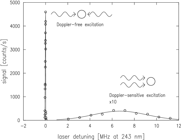
Figure 3: Composite $1S$-$2S$ spectrum of a thermal trapped hydrogen sample, showing both Doppler-free and Doppler-sensitive contributions. In the Doppler-free excitation mode, a hydrogen atom is promoted to the $2S$ state by absorbing counter-propagating 243 nm photons. Since there is no first-order Doppler-broadening, the corresponding spectral feature is narrow and intense. In the Doppler-sensitive excitation mode, where two co-propagating photons are absorbed, the spectrum is both recoil-shifted and Doppler-broadened.

3 Two-Photon $1S$-$2S$ Excitation

Excitation of the $1S$-$2S$ transition is accomplished using two 243 nm photons from a UV laser. The hydrogen $1S$-$2S$ spectrum has both Doppler-free and Doppler-sensitive resonances, separated by a recoil shift (see Fig. 3). Although the natural linewidth of the $1S$-$2S$ transition is only 0.65 Hz at 243 nm, the experimental Doppler-free linewidth is at least a few kilohertz due to a combination of transit-time broadening [30], finite laser linewidth, and the cold-collision frequency shift [2]. By comparison, the Doppler-sensitive line has a width of $\sim 4$ MHz at the coldest experimental temperatures, and the width grows with increasing temperature. To excite large numbers of metastables, the laser is tuned to the narrow, intense Doppler-free spectral feature.

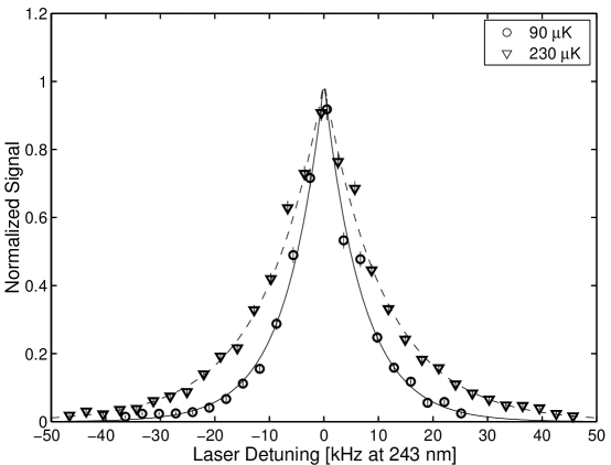
Figure 4: Examples of Doppler-free $1S$-$2S$ lineshapes for low-density $(\sim 10^{13}$cm${}^{-3})$ $1S$ samples at two different temperatures. At these densities, the width of the spectrum is dominated by transit-time broadening, and the lineshape is double-exponential, characteristic of Doppler-free two-photon excitation by a Gaussian laser beam.

The hallmark of the Doppler-free resonance is the cusp-like lineshape which arises in a thermal gas due to transit-time broadening. For the case of a perfectly collimated, Gaussian laser beam and a homogeneous gas density, it can be shown [33] that the Doppler-free line of the gas has a spectrum proportional to $e^{-|\Delta\nu_{L}|/\gamma_{o}(T)}$ where $\Delta\nu_{L}$ is the laser detuning from resonance and $\gamma_{o}(T)\propto\sqrt{T}$ is the $1/e$ half-width of the line. This lineshape is called “double-exponential” because it consists of two exponential functions meeting at a cusp. For temperatures at which the above criteria for gas density and laser collimation are approximately satisfied, the relative width of the Doppler line is a useful measure of relative sample temperature (Fig. 4) [30, 1]. Low sample densities must be employed to resolve these double-exponential lineshapes. At high $1S$ densities ($>10^{13}$ cm^-3), the $1S$-$2S$ cold-collision shift flattens the cusp and significantly broadens the line [2].

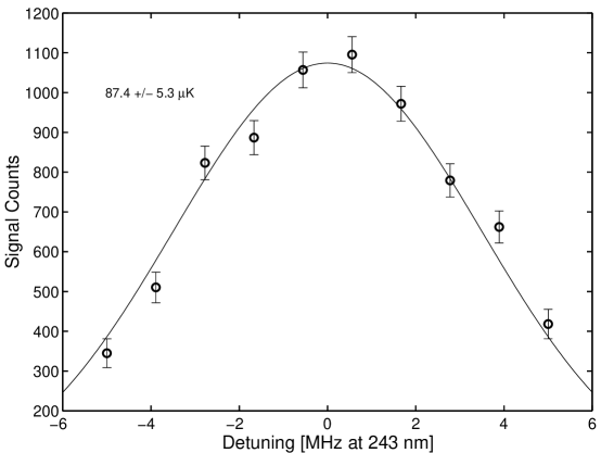
Figure 5: Temperature determination from a Gaussian fit to the Doppler-sensitive component of the H $1S$-$2S$ spectrum. In this example, spectroscopic data from six consecutive trap cycles are summed together.

The Doppler-sensitive spectrum (Fig. 5) is proportional to the momentum distribution of the sample along the direction of the excitation laser [34]. As long as the sample is not close to quantum degeneracy, the distribution is Maxwell-Boltzmann, and the lineshape is Gaussian; this is always the case for samples in this thesis. Like the Doppler-free double-exponential, the Doppler-sensitive width scales as $\sqrt{T}$. Unlike the Doppler-free case, the width is simply related to the absolute temperature and is independent of the laser and trap geometry. A Gaussian fit to the Doppler-sensitive spectrum provides the most direct way of calibrating the temperature of a trapped hydrogen sample. Unfortunately, at temperatures above $\sim 100$ $\mu$K the line is so broad and weak that, in our current apparatus, many trap cycles are required to accumulate enough statistics for a temperature measurement.

For more thorough and formal descriptions of $1S$-$2S$ excitation in hydrogen, see Refs. [35, 36, 37, 1].

4 Overview of the Thesis

The next chapter will begin by describing the experimental sequence applied to produce a cloud of trapped $2S$ atoms. The later sections of Ch. 1 focus on apparatus and techniques which have not yet been detailed in other theses and publications; these include the method for metastable decay measurements. Chapter 2 delves into several aspects of the physics of metastable H in a magnetic trap, mostly from a theoretical standpoint. Chapter 3 describes the magnetic trap configurations used in decay measurements and introduces data suggesting the presence of two-body loss in our metastable clouds. The analysis of decay data to calculate a $2S$-$2S$ loss rate constant and place limits on inelastic $1S$-$2S$ collision rates is presented in Ch. 4. In the concluding chapter, some suggestions are made for further experiments using the current apparatus and also for a new apparatus optimized for spectroscopy of metastable H.

Throughout this thesis, the term “$2S$” is used interchangeably with the term “metastable”; the same applies for “$1S$” and “ground state.”

Chapter 1 Apparatus and Experimental Techniques

The apparatus used for experiments described in this thesis was developed with two principal goals in mind: (1) observation of Bose-Einstein condensation in atomic hydrogen and (2) high resolution spectroscopy of ultracold hydrogen on the $1S$-$2S$ transition. These goals required the parallel development of a sophisticated cryogenic apparatus and a highly frequency-stable UV laser system. Many of the important developments have been described in other PhD theses from the MIT Ultracold Hydrogen Group [29, 36, 38, 39, 1]. This chapter will recapitulate the methods used to generate and probe ultracold hydrogen with emphasis on recent refinements. The first section provides an overview of the trap cycle used for measurements in this thesis, while the following sections discuss details of our techniques which, for the most part, have not been recorded elsewhere.

1 A Typical Trap Cycle

Samples of atomic hydrogen are generated, trapped, cooled, and probed in a cycle lasting typically 5–15 minutes depending on the desired final sample temperature and type of measurement. At the beginning of each cycle, pulses of rf power are supplied to a copper coil in a cylindrical resonator [1] which is thermally anchored (Fig. 1) to the mixing chamber of a dilution refrigerator. The resulting rf discharge vaporizes and dissociates frozen molecular hydrogen from surfaces in the resonator. Atoms in all four $1S$ hyperfine states are injected into a trapping cell. The two high field seeking states ($a$ and $b$) are drawn back to the 4 T magnetic field in the discharge region, while the low field seekers ($c$ and $d$) are attracted to the 0.6 K deep Ioffe-Pritchard magnetic trap [32] in the trapping cell (see Figs. 4 and 5).

In order for trapping to be successful, a sufficiently thick film of superfluid He must coat the walls of the cell. The low field seekers are cooled initially by interaction with the cell walls. While the discharge operates, the cell is held at a temperature of 320 mK, which is warm enough for the residence time of H atoms on the He film to be shorter than the time it takes for atoms to spin-flip on the walls, and cold enough for a sizeable fraction of H atoms to settle into the trap after exchanging energy in elastic collisions [29]. The $c$-state atoms disappear in a few seconds due to spin-exchange collisions, and a pure $d$-state ($F=1$, $m_{F}=1$) gas remains in the trap. After the loading period is finished, the cell is rapidly cooled to below 100 mK by the dilution refrigerator. At this temperature, atoms with enough energy to reach the walls are permanently lost from the trapped sample. Evaporative cooling begins, and the sample becomes thermally disconnected from the cell. Once thermal disconnect is complete, the atom cloud equilibrates at a temperature of typically 40 mK.

The threshold energy of the magnetic trap is determined by a saddlepoint of the magnetic field at one end of the trap. Atoms with energy above threshold can escape over the saddlepoint, leading to evaporative cooling of the sample. By progressively lowering the saddlepoint field, evaporation is forced. In this way, the sample can be cooled to temperatures as low as $\sim 200$ $\mu$K in 4-5 minutes.

In order to reach sample temperatures down to $\sim 20$ $\mu$K, rf evaporation is employed. For a given rf frequency $\nu_{\rm rf}$, there is a three-dimensional “surface of death” consisting of all points having a magnetic field such that the $d$-$c$ and $c$-$b$ hyperfine transitions of the atoms are resonant. Atoms with energy greater than $h\nu_{\rm rf}$ can cross the surface of death several times per millisecond and quickly transition to an untrapped state. Thus, $\nu_{\rm rf}$ sets an efficient threshold for the trap. The coldest temperatures in the MIT hydrogen experiment are achieved by ramping $\nu_{\rm rf}$ from 35 MHz (significantly above the magnetic trap threshold) to the desired final threshold value, usually between 5 and 20 MHz (240 and 960 $\mu$K).

The dramatic cooling of the sample by several orders of magnitude in temperature is accomplished at the expense of atom number. The magnetic trap, initially loaded with $\sim 10^{14}$ atoms, contains only $\sim 10^{11}$ atoms at the 200 $\mu$K limit of magnetic saddlepoint evaporation and fewer than $10^{10}$ atoms at the lowest temperatures accessible by rf evaporation.

Atoms are lost during the trap cycle not only to evaporation but also to two-body “dipolar” decay collisions [40]. These are $d+d$ collisions in which the magnetic dipole interaction causes at least one of the two atoms to change spin state. They occur preferentially in the highest density region of the sample, where the average energy of an atom is less than $kT$. Thus dipolar decay leads to heating of the sample. To maintain a favorable ratio of elastic to inelastic collisions, the radially confining fields are reduced simultaneously with the saddlepoint field to prevent the atom density from growing significantly as the temperature drops. During rf evaporation, however, the peak density grows rapidly, and dipolar losses set a limit on the temperature which can be reached.

For experiments with metastable hydrogen, the last phase of the trap cycle involves repeated two-photon excitation of the ground state sample with a 243 nm UV laser nearly resonant with the Doppler-free $1S$-$2S$ transition. A typical excitation pulse lasts $1\sim 3$ ms. The resulting $2S$ atoms are quenched by an electric field pulse after a wait time of up to 100 ms; these quenched atoms are mostly lost from the trap [36]. However, the quenching process also results in Lyman-$\alpha$ fluorescence photons, some of which are detected on a microchannel plate (MCP) detector. The number of signal counts recorded is proportional to the number of metastables present at the time of quenching. Typically, $\sim 10^{8}$ or fewer $2S$ atoms are excited per laser pulse. Thus, metastable clouds can be generated hundreds of times with different wait times and laser frequencies before depleting the ground state sample.

For measurements on the ground state atoms, two methods of probing are available. First, there is conventional $1S$-$2S$ excitation spectroscopy [30, 1], already introduced in Ch. Studies with Ultracold Metastable Hydrogen. In this mode of taking data, the laser is typically chopped at 100 Hz with a 10% duty cycle, and a quenching electric field pulse is applied at a fixed time of $\sim 6$ ms after excitation. The laser frequency is stepped back and forth across a specified range, each sweep of the range lasting less than 1 s. This provides a series of snapshots in time of some portion of the $1S$-$2S$ spectrum. The spectroscopic data provides crucial information about the sample (see Ch. Studies with Ultracold Metastable Hydrogen). At higher sample densities, the broadening of the Doppler-free line due to the cold-collision shift provides information about the density distribution of the sample. At low densities, the Doppler-free width is proportional to the square root of the temperature. At low temperatures, the width of the Doppler-sensitive line is an excellent measure of absolute temperature.

The second and older method of probing the ground state sample involves “dumping” the atoms from the trap and detecting the recombination heat on a bolometer [29]. This method involves rapidly lowering the saddlepoint magnetic barrier, allowing the atoms to escape to a zero field region and/or forming a zero field region in the trap. The atoms quickly spin-flip and recombine. The integral of the resulting bolometer signal is proportional to the number of atoms in the trap. An important application of this technique is the determination of initial sample density from the decay in $1S$ number due to dipolar loss (Sec. 3).

Throughout the trap cycle a dedicated computer controls the necessary power supplies, frequency sources, relays, heaters, and data acquisition electronics.

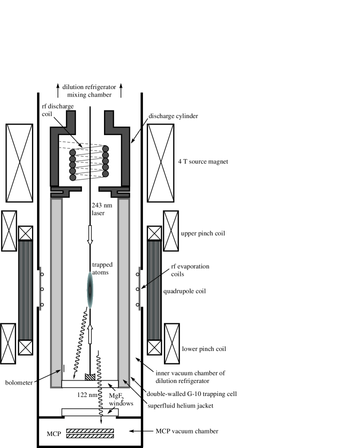
Figure 1: Cartoon of cryogenic apparatus, not to scale: the ratio of the length of the trapping cell ($\sim 65$ cm) to its inner diameter (4 cm) is much larger than depicted here. During the loading phase, atoms accumulate in a Ioffe-Pritchard trap with radial confinement provided by an elongated set of quadrupole coils and axial confinement by two “pinch” coils. As the sample is evaporatively cooled, the fields of other smaller, fine-control magnets come into play. All the magnets are immersed in liquid helium and are superconducting.

2 Enhancements to the Cryogenic Apparatus

In 1998, our group successfully demonstrated rf evaporation in a cryogenic trapping apparatus. The enabling technology was a new nonmetallic trapping cell consisting of two concentric G-10 tubes [39]. By eliminating metal parts from the cell, sufficient rf power for evaporation could be delivered to coils wrapped directly on the inner G-10 tube without placing an excessive heat load on the dilution refrigerator. In the nonmetallic design, heat transport to the mixing chamber was provided by filling the volume between the tubes with superfluid helium.

The cryogenic trapping cell used for experiments described in this thesis represents a second-generation nonmetallic design. A major problem of the first-generation G-10 cell was the presence of relatively large stray electric fields ($\sim 500$ mV/cm) which limited metastable lifetimes to between a few hundred microseconds and a few milliseconds. Worse yet, the stray fields sometimes changed unpredictably on a time scale of minutes. Many spectroscopy runs were rendered almost useless by these fields. Furthermore, since short $2S$ lifetimes did not afford the opportunity to wait for laser-induced background fluorescence to die away after excitation, the stray fields limited the signal-to-noise ratio in $1S$-$2S$ spectroscopy. The problem of stray fields was solved in the second-generation G-10 cell by adding a thin copper film to the inside cell wall. This film was thin enough to avoid significant absorption of rf power, yet thick enough to suppress stray fields to the 40 mV/cm level. With the copper film, $2S$ lifetimes in excess of 80 ms have been observed, and the stability of stray fields is much improved. Since the film is divided into several externally controllable electrodes, partial compensation of the residual stray fields is possible (Sec. 5).

Another change in the second-generation design was the relocation of rf evaporation coils to the inner vacuum chamber (IVC) “tailpiece,” which separates the surrounding magnets and liquid helium bath at 4 K from the vacuum space containing the trapping cell. In the first-generation G-10 cell, the heat load on the dilution refrigerator due to the evaporation coil leads placed a limit on the allowable rf drive power. Furthermore, intolerable heating of the cell occurred at absorptive resonances above 25 MHz. By thermally anchoring the coils to the 4 K bath instead of the dilution refrigerator, heating of the rf leads was no longer a limitation. The absorptive resonances were also shifted such that rf evaporation could occur in a continuous downward sweep from 35 MHz. This permits more efficient rf evaporation and may also enable better shielding of the sample from a high-energy atom “Oort cloud” which forms during magnetic saddlepoint evaporation [41, 42]. To accomplish relocation of the coils, the middle portion of the brass IVC tailpiece was replaced by a G-10 section of slightly smaller diameter. The nonmetallic section was necessary to allow propagation of the rf from the coils to the atoms.

In the second-generation design, minor changes were made to the geometry of the detection end of the trapping cell, slightly increasing the solid angle of detection. Further details on the construction of the current cryogenic apparatus are given by Moss [43].

The introduction of a nonmetallic trapping cell allowing rf evaporation in a cryogenic environment was not only necessary for the achievement of BEC, but also enabled us to generate higher densities of metastables than ever before. These higher densities, together with the addition of electrical shielding to the “plastic” G-10 tube, were crucial prerequisites for the observation of two-body metastable loss described in Chapters 3 and 4.

3 The Bolometer

1 Construction

The current bolometer design is a refinement of those described in the theses of Yu [44] and Doyle [29]. Following a suggestion of D. G. Fried, the area of the electrodes was reduced to ameliorate rf pickup. A new construction method was developed after thermal cycling tests with different glues and wire-bonding methods, and it has proven to be highly robust against thermal stress and mechanical shock. For the benefit of those wishing to construct such a bolometer themselves, a detailed description of this important diagnostic device is presented here.

The ideal bolometer has a very small heat capacity, good internal thermal conductivity, and good thermal and electrical isolation from its surroundings. Quartz was chosen as the substrate because its heat capacity at millikelvin temperatures is tiny, it has sufficient thermal conductivity, and it is commercially available in very thin plates. The current bolometer substrate is a chemically polished plate (1 cm $\times$ 1 cm $\times$ 50 $\mu$m) [45]. The heat capacity of the substrate is probably only a few percent of the total bolometer heat capacity (roughly $\sim 10^{-8}$ J/K at 350 mK), which is likely dominated by amorphous graphite patches (Fig. 2(a)) and the superfluid film which is ubiquitous in the trapping cell. The time resolution of the bolometer is limited ultimately by the time it takes for heat deposited at one point on its surface to spread throughout its bulk. An upper limit on the time constant for this spreading, $\tau_{s}$, is obtained by dividing the heat capacity by the thermal conductivity between two edges of the quartz plate. At a typical operating temperature of 350 mK, the result is $\tau_{s}<40$ $\mu$s. A detection bandwidth of several kilohertz has been demonstrated with the bolometer described here. For most measurements, however, a low-pass filter is used to suppress 60 Hz and other noise pickup in the sensitive bolometer circuit.

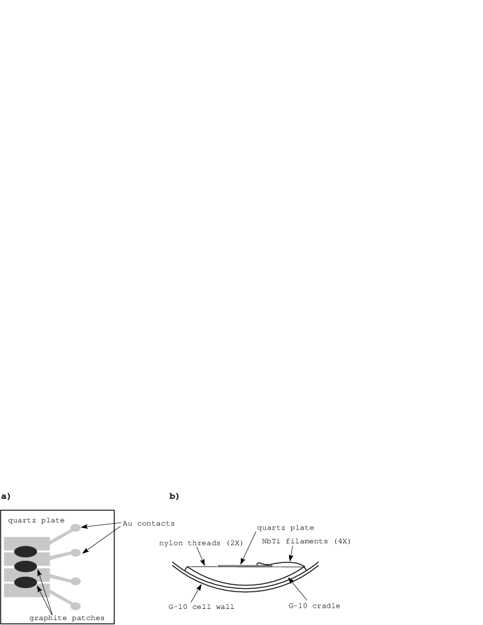
Figure 2: (a) Face view of quartz bolometer. The NbTi filament leads, which are bonded to the circular ends of the Au contact pads, are omitted. (b) Edge view showing bolometer suspended from its cradle and a filament lead.

A physical mask was made for the electrode pattern by cutting an aperture in a thin metal plate and soldering three $\sim 38$ $\mu$m diameter wires across the aperture. An evaporator was used to deposit 5 nm of chromium followed by 100 nm of gold onto the quartz. The resulting pattern is shown in Fig. 2(a). Electrical leads were bonded to the gold pads using silver epoxy to establish good electrical contact, while droplets of Stycast 1266 epoxy [46] near the edge of the plate provided a strong mechanical bond between the leads and the quartz (see Fig. 2(b)). To avoid adding unnecessary heat capacity to the bolometer in the form of excess epoxy, the droplets were applied with the end of a fine wire. To minimize the thermal link between bolometer and cell, 30 $\mu$m diameter superconducting NbTi filaments were used as electrical leads. These filaments were obtained by dissolving the copper matrix of a multi-filament magnet wire in nitric acid.

Across the gaps between gold pads, amorphous graphite resistors were deposited by repeated applications of Aerodag [47]. The graphite patches have resistances of $1$-$2$ k$\Omega$ at room temperature, but increase to several tens of k$\Omega$ below 300 mK. In practice, only two electrical connections and one resistor is used at a time; the others provide redundancy in case of a failure. As explained below, the resistor serves as both temperature sensor and heater.

The quartz plate was laid across two nylon threads, about 10 $\mu$m in diameter, which were stretched taut across a G-10 cradle piece having the same radius of curvature as the inside of the cell. Small drops of Stycast 1266 were allowed to wick along the threads, providing a large-surface-area bond between the threads and quartz plate. The G-10 cradle was then mounted by epoxy on the cell wall so that the bolometer sits vertically below the magnetic trap.

2 Operation

In typical operation, the bolometer is held at a temperature between 200 mK and 350 mK, considerably above the cell wall temperature in the later stages of the trap cycle. The bolometer acts as a “thermistor” in a resistance bridge feedback circuit; its temperature setpoint is determined by a variable resistor outside of the cryostat. A signal is derived by amplifying the changes in feedback voltage required to hold the bolometer at constant temperature. This feedback mode of operation allows for much higher linearity and bandwidth than simply monitoring changes in the bolometer resistance. Different temperature setpoints are selected depending on the type of bolometric measurement; the bolometer is more sensitive at lower temperatures because heat capacity is lower, and the temperature coefficient of its resistance is larger.

The primary purpose of the bolometer in our apparatus is to detect the recombination heat released when atoms from the trap are allowed to reach the cell wall or spin-flip at a zero of the magnetic field. The resulting H₂ molecules retain much of the 4.6 eV recombination energy in their rovibrational degrees of freedom [48]. Since the molecules are insensitive to the magnetic field, they bounce freely around the cell, transferring some of their energy in collisions with surfaces. In this way, a small fraction of the recombination energy reaches the bolometer. Doyle estimated this fraction to be $4\times 10^{-4}$ for a similar bolometer [29]. Operating at a temperature of $\sim 200\mu$K, the current bolometer is sensitive enough to detect a flux of $\sim 10^{9}$ atoms/s. If Doyle’s fraction is still appropriate, this flux corresponds to a power of $\sim 10^{-13}$ W at the bolometer.

3 Density Measurements

As mentioned in Sec. 2, the relative number of atoms in the trap can be determined by dumping the atoms from the trap and integrating the bolometer signal. Since the atom number after loading and evaporation processes is reproducible to a few percent in successive trap cycles, it is possible to map out the decay curve of an equilibrium sample by waiting different lengths of time before dumping. From the local equation for dipolar density decay,

$$\frac{dn_{1S}}{dt}=-gn_{1S}^{2},$$ (1)

it is possible to derive the following equation involving atom number $N_{1S}$ as a function of time:

$$\frac{N_{1S}(0)}{N_{1S}(t)}=1+(1+\xi f)\frac{Q_{1S}(T)}{V_{1S}(T)}gn_{1S,o}(0)t.$$ (2)

Here, $n_{1S,o}$ is the peak density in the trap, and $g=1.2\times 10^{-15}$ cm²/s is the theoretical rate coefficient for dipolar decay of $d$-state atoms[40]. The quantity $V_{1S}$ is known as the effective volume and is defined as the ratio $N_{1S}/n_{1S,o}$. It can also be expressed in terms of the normalized spatial distribution function $f_{1S}({\bf r})=n_{1S}({\bf r})/n_{1S,o}$: $V_{1S}=\int f_{1S}({\bf r})d^{3}{\bf r}$. The quantity $Q_{1S}=\int f^{2}_{1S}({\bf r})d^{3}{\bf r}$ can be considered the effective volume for two-body loss. Both $V_{1S}$ and $Q_{1S}$ depend on the temperature $T$. The factor $(1+\xi f)$ is a correction factor accounting for the fact that some evaporation must occur simultaneously with dipolar decay if the sample is in equilibrium. More specifically, $\xi$ represents the ratio of elastic collisions to inelastic collisions, and $f$ is the fraction of elastic collisions which result in an atom leaving the trap.

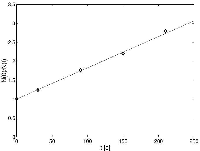
Figure 3: Inverse of integrated bolometer signal, normalized to its value at $t=0$, when dumping atoms after different wait times $t$. The example shown here is for a sample in Trap Y of Ch. 3. The initial peak density derived from the linear fit is $2.4\times 10^{13}$ cm^-3.

Equation 2 describes the time-dependence of the inverse normalized atom number, $N_{1S}(0)/N_{1S}(t)$. This can be determined from integrated bolometer signals without knowing the bolometer detection efficiency. As shown in Fig. 3, the inverse atom number has a linear time dependence, characteristic of two-body decay. The slope of $N_{1S}(0)/N_{1S}(t)$ can be used to determine the initial density $n_{1S,o}$ assuming the other quantities are well known. The theoretical value of $g$ is believed accurate to better than 10% [49]. Furthermore, the ratio $Q_{1S}/V_{1S}$ can be calculated numerically from the known geometry of the magnets to about 10%. The uncertainty stems from both imperfect knowledge of the trapping field and uncertainty in the sample temperature.

From thermodynamic considerations, it can be shown that the evaporation correction factor is given by [50]

$$(1+\xi f)=\frac{\eta+\beta-3/2-\delta/2}{\eta+\beta-3/2-\delta}.$$ (3)

In this equation, $\eta$ is the ratio of trap depth to temperature ($8<\eta<11$ for samples analyzed in this thesis); $\beta$ is the average fraction of thermal energy $kT$ carried away by an evaporated atom in excess of the the threshold energy $\eta kT$. Numerical calculations by the MIT group as well as theoretical calculations by the Amsterdam group [51] have shown that $\beta\simeq 0.8$ for the range of $\eta$ found in our experiment, assuming a cylindrical quadrupole trap. The constant $\delta$, defined by $dV_{1S}\propto U^{\delta-1}dU$, where $U$ is potential energy, is equal to 2 for a cylindrical quadrupole trap, 1 for a cylindrical harmonic trap, and 3 for a spherical quadrupole trap. For the traps relevant here, it is a good approximation to take $\delta=2$, and Eq. 3 simplifies to

$$(1+\xi f)\simeq\frac{\eta-1.7}{\eta-2.7}.$$ (4)

This expression is believed accurate to a few percent for all but the coldest samples in the MIT hydrogen experiment. (An alternative approach to calculating the correction factor is outlined in [51, 39]). Depending on $\eta$, which generally decreases as the sample temperature decreases, the evaporation correction amounts to a 10-20% reduction in the apparent density.

The uncertainties in $g$, the evaporation correction factor, and the effective volumes are the dominant contributions to the error in ground state density measurements. By adding these contributions in quadrature, the total uncertainty is estimated to be about 20%.

4 Loading the Magnetic Trap

Over the past several years, a number of studies have been undertaken to better understand what is arguably the most physically complex stage of the trapping cycle: the loading phase. The goal of these studies has been to understand what limits the number of atoms which can be accumulated in our trap. This section summarizes the current state of knowledge about the physics of hydrogen trap loading, highlighting our recent investigations.

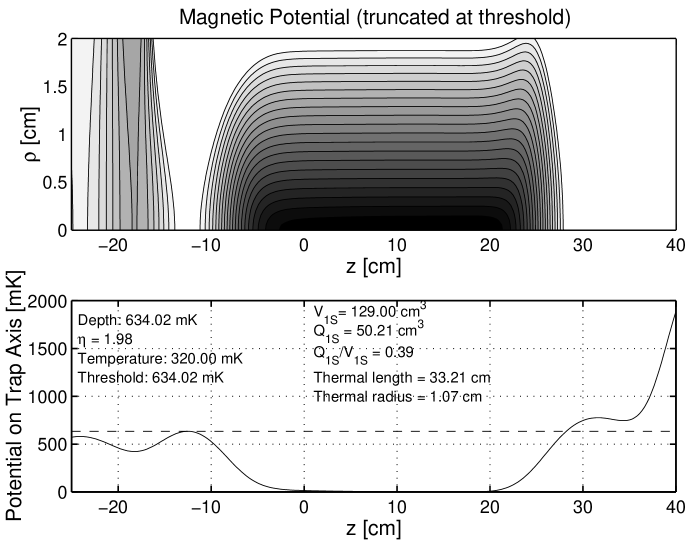
Figure 4: Trap shape during accumulation; the sample temperature is determined by the 320 mK cell wall temperature. The trap volumes are calculated assuming a truncated Maxwell-Boltzmann distribution. The leftmost edge of the plots correspond to the MgF₂ window at the bottom of the trapping cell (see Fig. 1), and the cell wall is at $\rho=1.9$ cm. Local maxima of the field on axis near $z=-24,-12,+32$ cm result from contributions by the loading, lower pinch, and upper pinch magnets, respectively. See also Fig. 5.

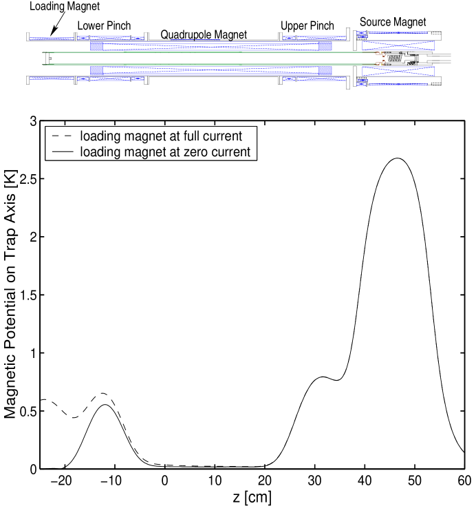
Figure 5: Magnetic field profile along the trap axis showing the 4 T (2.7 K) source field in the discharge resonator. Atoms in all four $1S$ hyperfine states are generated in the high source field and stream into the lower field regions. After thermalizing with the cell walls, $d$-state atoms settle into the trap between $z=-10$ and $z=25$ cm. Once accumulation is complete, the loading magnet current is ramped to zero. At top and aligned with the magnetic field profile is a CAD drawing of the principal magnets and trapping cell.

The loading phase can be divided into two parts: accumulation and thermal disconnect. In preparation for accumulation, the largest of the computer-controlled magnets are ramped to maximum current, generating a 0.6 K deep Ioffe-Pritchard trap. At this time, a “loading magnet” is energized to prevent the existence of a zero field region near the lower end of the trapping cell (Figs. 4 and 5). In the next few seconds, the cell is heated above 300 mK by heaters inside the superfluid helium jacket, making the cell walls less “sticky.” At this temperature, atoms are adsorbed on the helium film for less than 1 $\mu$s before returning to the gas [29]. (The binding energy for hydrogen atoms on superfluid helium is about 1 K [52]). Once the cell is sufficiently warm, discharge pulses begin puffing atoms into the trapping cell, at a typical pulse rate of 50 Hz. The atoms thermalize with the walls and explore the entire cell volume. The population of $d$-state atoms in the magnetic trap region grows to a saturation value. While the discharge pulses feed this population, a number of loss processes can occur, including dipolar decay and other two-body inelastic collisions in the gas, one-body spin-flips on the cell walls, and two-body recombination on the walls. As will be explained below, however, most of these processes can be ruled out as the limiting factor in determining how many atoms are trapped.

When accumulation is complete, the cell heater is switched off, and the cell temperature drops below 150 mK in about 2 s. After about 10 s, the temperature reaches 100 mK. During the rapid cooldown, the flux of atoms to the wall from the magnetic trap minimum decreases. However, the residence time of atoms on the walls dramatically increases, and the relatively slow wall loss processes begin to remove atoms with enough energy to reach the wall. When the cell passes through a temperature of roughly 150 mK, the magnetically trapped sample thermally disconnects from the walls; the probability of atoms returning from the walls goes to zero. Meanwhile, the sample continues to cool by evaporation of atoms to the walls, and its temperature drops below the wall temperature. In a typical trap cycle, the loading magnet is ramped down simultaneously with thermal disconnect, and evaporation over the magnetic saddlepoint begins. About $1\times 10^{14}$ atoms equilibrate at a temperature of 40 mK and a peak density of $2\times 10^{13}$ cm^-3.

The primary means for studying the loading process is to introduce variations in the sequence and observe the effect on atom number. The atoms can be dumped directly from the initial deep magnetic trap and detected on the bolometer.

1 Pulsed Discharge

The 300 MHz discharge resonator currently in use is described by Killian [1]. Several studies were performed to optimize the duty cycle, pulse length, and rf power parameters of the discharge. These studies show that all of these parameters can be varied over a wide range without changing the saturation atom number by more than a few percent. The time constant for reaching saturation, however, depends on the average power supplied to the discharge.

For constant rf power, it was found that larger duty cycles result in more atoms trapped per unit energy supplied to the discharge. An energy efficient discharge is desirable since it requires less heat to be removed from the copper resonator by the dilution refrigerator. As will be explained in Sec. 4, maximum cooling power is desired during thermal disconnect. Very short $(<100$ $\mu$s) discharge pulses are inefficient because it takes 15-25 $\mu$s for the discharge to start firing after the beginning of each rf pulse. The energy deposited in the resonator during this time heats the fridge but does not produce atoms. The reason for this “dead time” may be that sufficient helium vapor pressure must develop in the resonator before discharge activity can begin.

Some effort was expended to optimize the shape of the rf pulses. An rf switching scheme was used to apply two different power levels, a lower level during the dead time (25 $\mu$s) and a 5-9 dB higher level during the firing time (100 $\mu$s-10 ms) of each pulse. Typical peak powers at the amplifier output driving the discharge were 50-100 W, applied at duty cycles of 0.5-5%. The bolometer was used to record atom pulses as the discharge was firing. Also, studies were made of the trapped atom number as a function of accumulation time. A number of different pulse lengths and power levels were tried. Although the size of the atom pulses scaled linearly with the product of RF power and firing time, it was found that almost regardless of pulse characteristics the trapped atom number after thermal disconnect saturated at nearly the same value. A couple conclusions were drawn from these studies. First, the trapped atom number is not limited by the number of atoms produced in a single discharge pulse. Second, since we were unable to trap more atoms using attenuated rf power during the dead time of each pulse, it seems that overheating of the resonator is not the number-limiting factor. The power switching scheme provided no clear advantage.

Even though the saturation atom number is not better, a high average flux from the discharge is desirable because it shortens the accumulation time. This means less total heat is required to hold the cell at its relatively high accumulation temperature; after the loading phase the cell can more quickly reach a cold temperature advantageous for sensitive bolometric detection. For the experiments described in the remainder of this thesis, discharge parameters were chosen which loaded the trap 3-4 times faster than in the initial nonmetallic cell experiments. Typically, the discharge operates with 1 ms pulses repeated at 50 Hz for a total of 8 s. The peak power of the (square) rf pulses at the amplifier output is $\sim 90$ W.

A sufficient helium film thickness is important for efficient loading of the trap from the discharge. If the the film is too thin, bare spots can form in the cell and resonator while the discharge fires. The bare spots serve as sticky sites where atoms spin-flip and recombine. The discharge itself can become erratic with a very thin film, probably due to low vapor pressure in the resonator.

2 The Accumulating Sample

The discharge injects a flux of both high field and low field seekers into the trapping cell. The average flux (counting only $d$ states) is more than 10¹³ atoms/s, and a single 1 ms pulse may inject nearly 10¹² atoms. The high field seeking $a$ and $b$ states are eventually pulled back toward the 2.7 K source field (Fig. 5), though this can take some time if they reach the trap region and equilibrate with the wall. In the trap region, the gradient in $z$ is low, and high field seekers bounce randomly on the cell wall until reaching the high gradient in $z$. From the ratio of the cell wall area in this region to the cell cross-section, we can estimate that the the atoms must bounce 25 times before leaving the low-gradient region. At 300 mK, the average time between bounces is about 1 ms, implying a time constant of $\tau_{\rm hf}\sim 25$ ms for high field seekers to return to the source. High field seekers reaching the relatively high field at the opposite end of the trap may linger there and take even longer to return. In the meantime, the high field seekers can undergo hyperfine-changing collisions with $d$ atoms, potentially causing trap loss.

The other low field seekers, $c$-state atoms, disappear due to spin exchange collisions on a time scale of seconds. As a result, the sample becomes purely $d$-state within seconds after the end of accumulation.

Some insight was gained from studies in which the bolometer was deliberately made bare of helium film for a time during or after accumulation. This was accomplished by applying several hundred microamps to the bolometer. When the bolometer was bare throughout accumulation, the number of atoms loaded into the trap was reduced by nearly two orders of magnitude. What is more, the number remaining depended on the magnetic potential $E_{\rm bolo}$ at the bolometer, which sits at approximately $z=-23$ cm in the coordinate system of the Figures. We varied $E_{\rm bolo}$ using the loading magnet current. Under the assumption that the bare bolometer surface was the dominant loss mechanism during loading, the dependence of the atom number on $E_{\rm bolo}$ was found roughly consistent with a thermally distributed sample at the cell temperature. Furthermore, it was found that the sample could be depleted by baring the bolometer at a time long after the discharge stopped firing as long as the cell temperature was maintained. If the bolometer was not bared, then the sample could be held at the cell temperature for 30 s or more after accumulation without significant depletion. Finally, if the cell was allowed to cool after accumulation, a subsequent baring of the bolometer had no effect on the atom number. This was interpreted as a signature of thermal disconnect.

These observations provided evidence that the assumption of the accumulating sample being in equilibrium at the cell temperature is a good one. In addition, we found evidence that the peak trap density reaches a saturation value during accumulation which is too low for significant loss due to dipolar decay. Since the evaporation process during thermal disconnect is believed to be well understood (Sec. 4), measurements of atom number following thermal disconnect allow an order of magnitude estimate of the sample density before thermal disconnect. These measurements led to the conclusion that the peak loading density is $(\sim 10^{12}$ cm^-3$)$, at which the decay time due to dipolar decay is many minutes. The fact that the atom number after thermal disconnect does not change appreciably when the atoms are held for many seconds at the loading temperature following accumulation also suggests a low density at the end of accumulation. This would mean that the key limiting process during loading occurs in the accumulation phase. However, in the absence of more direct measurements of the density before thermal disconnect, we admit the possibility that an unknown process during thermal disconnect may cap the atom number at a definite maximum.

If indeed the sample can be held in thermal contact with the walls for many seconds without loss, an implication is that surface loss processes at the cell loading temperature are not important for a $d$-state sample. In other words, one-body spin flip and surface recombination are not limiting processes during accumulation.

Since the bolometer is the most poorly thermally anchored part of the trapping cell, there was some concern that the bolometer was heating enough to become bare while the discharge was firing even under normal circumstances. This possibility was ruled out by the bare bolometer studies.

One unexpected observation was that the time to reach saturation number in the trap was unaffected by the bare bolometer. This implies that there is another loss mechanism other than the bare bolometer which was determining the saturation atom number in the above studies.

3 Phenomenological Model

We will assume for the moment that the most important loss mechanism occurs during accumulation. The fact that the saturation atom number is independent of discharge pulse parameters suggests a phenomenological model for trap loading which involves a loss rate proportional to the discharge flux. Consider the simple model

$$\frac{dN_{d}}{dt}=F_{d}-\beta F_{d}N_{d},$$ (5)

where $N_{d}$ is the number of $d$ atoms in the trap, $F_{d}$ is the average flux of $d$ atoms from the discharge, including $d$ atoms resulting from hyperfine-changing collisions, and $\beta$ is a proportionality constant for the dominant loss mechanism. The solution to Eq. 5 is

$$N_{d}(t)=\frac{1}{\beta}(1-e^{-\beta F_{d}t}).$$ (6)

The saturation time constant $\tau_{\rm sat}=(\beta F_{d})^{-1}$ depends inversely on the average flux, consistent with data from discharge parameter studies. In addition, the saturation value depends only on $\beta$ and not the flux. The question remains: what physical process gives rise to $\beta$?

One candidate is the inelastic collisions between $d$ atoms and high field seekers in the thermal gas during the time $\tau_{\rm hf}$ after a discharge pulse (Sec. 2). According to theoretical calculations [40], there are several $b+d$ inelastic processes with large cross sections. The channels $b+d\rightarrow a+a$ and $b+d\rightarrow c+c$, for example, both have rate coefficients of approximately $4\times 10^{-13}$ cm³/s at 300 mK and zero field. Rate coefficients for $a+d$ processes have not been calculated at finite temperature, but in the zero temperature limit, the rate coefficients of the most likely $a+d$ channels are several orders of magnitude below the $b+d$ channels at all magnetic fields. Taking $b+d$ collisions to be the dominant source of loss, the local rate of $d$-state density change due to collisions with high field seekers can be expressed

$$\left.\frac{dn_{d}}{dt}\right|_{\rm loss}=-g_{bd}n_{b}n_{d},$$ (7)

where $g_{bd}$ is the local total loss rate constant for $b+d$ collisions, and $n_{d}$ and $n_{b}$ are the $d$ and $b$ atom densities, respectively. The rate constant is a function of position because it depends on the magnetic field. Using equilibrium distributions for the atoms, the rate of change of $d$-state number during accumulation is

$$\frac{dN_{d}}{dt}=F_{d}-\frac{N_{b}}{V_{d}V_{b}}\left(\int g_{bd}({\bf r})d^{3}{\bf r}\right)N_{d},$$ (8)

where $N_{b}$ is the total number of $b$ atoms in the trapping cell which are not already accelerating in a high gradient region back to the source; $V_{d}=\int{\rm exp}(-U({\bf r})/kT)d^{3}{\bf r}$ and $V_{b}=\int{\rm exp}(+U({\bf r})/kT)d^{3}{\bf r}$ are effective volumes for low field and high field seekers, respectively. The integration is to be taken over the cell volume occupied by the quasi-static $b$-state population $N_{b}$. From comparison of Eq. 8 with Eq. 5, we have

$$\tau_{\rm sat}=(\beta F_{d})^{-1}=\frac{V_{d}V_{b}}{N_{b}(\int g_{bd}({\bf r})d^{3}{\bf r})}.$$ (9)

To test the plausibility of this physical model, we plug some numbers into Eq. 9 and compare it with an observed time constant for saturation of $N_{d}$. Since this is an order of magnitude calculation, we arbitrarily take the integration volume to be the entire cell volume excluding the region of large gradient at $z>36$ cm. At 320 mK, numerical integration yields $V_{d}\simeq 150$ cm³ and $V_{b}\simeq 4000$ cm³. For the currently preferred discharge parameters, $\tau_{\rm sat}$ is observed to be $\sim 4$ s. Since there are about $1\times 10^{14}$ atoms accumulated in the trap, $\beta\simeq 1\times 10^{-14}$, implying $F_{d}\simeq 3\times 10^{13}$ s^-1. The discharge fires at 50 Hz, so each pulse brings about $6\times 10^{11}$ $d$ atoms into the cell. The discharge pulses are separated by a time comparable to $\tau_{\rm hf}$. If the number of $b$ atoms per pulse is not too different from the number of $d$ atoms, then $N_{b}$ is $\sim 10^{11}$. If we further assume that $g_{bd}$ averaged over the cell is $~{}10^{-12}$ cm³/s, the result is $(\beta F_{d})^{-1}\sim 10^{4}$ s, which is 3-4 orders of magnitude too long. It seems unlikely that either $g_{bd}$ or $N_{b}$ have been grossly underestimated here. In other words, $b+d$ collisions in the gas probably do not cause the observed saturation of $N_{d}$.

Inelastic $c+d$ collisions are another possibility. However, the rate coefficients for $c+d$ channels are probably far smaller than the $c+c$ channels which remove $c$ atoms from the trap. At zero temperature, the sum of theoretical $c+d$ rate coefficients is comparable to the sum of rate coefficients for $d+d$ processes, which are known not to cause significant loss during loading.

Not only the gas densities but also the surface densities of the four hyperfine states should be proportional to the discharge flux. For state $i$, the equilibrium surface density $\sigma_{i}$ is given by

$$\sigma_{i}=n_{i,{\rm w}}\lambda_{\rm dB}e^{E_{b}/kT},$$ (10)

where $n_{i,{\rm w}}$ is the gas density of species $i$ near the wall, $\lambda_{\rm dB}$ is the thermal deBroglie wavelength, and $E_{b}$ is the binding energy on the film. Can inelastic processes on the helium surface give rise to the loss term in the phenomenological model? Loading studies with different film thicknesses have shown that as long as the helium film is not too thin, the saturation atom number is about the same. Since changing the film thickness changes the binding energy of the hydrogen atoms on the surface, the rate of surface collisions should be affected by changing the film thickness. Thus, it also seems unlikely that inelastic surface collisions limit the atom number.

Another idea for a loss mechanism proportional to discharge flux is that high energy particles from the discharge knock $d$ atoms out of the trap. The discharge likely produces many other species besides the $1S$ hyperfine states of H. These could include metastable H, excited states of He, molecular states of H, and various ions. As these other species stream through the trapping region, they could cause loss of $d$ states.

To see if direct flux from the discharge causes loss, in one experimental run a series of baffles was installed in the opening between the discharge resonator and cell volume. The baffles were made of copper and were thermally anchored to the copper resonator. They were constructed such that any particles leaving the discharge would have to bounce several times on a cold, helium-covered surface before entering the cell. Most of the species mentioned above would not be able to bounce because of their relatively large surface binding energies. Furthermore, any particles streaming into the cell would have energies determined by the cold baffles rather than the discharge. The trap loading behavior was found, however, to be very similar to loading without the baffles. The maximum number of atoms loaded was again the same. We concluded that energetic particles from the discharge were not limiting the atom number.

Since the baffles were located in a high field gradient, the baffle studies also provided experimental evidence that high field seekers do not cause significant loss during loading. The baffles should have prevented most high field seekers from reaching the trap, and yet the saturation behavior of loading was unchanged.

4 Thermal Disconnect

Some light was shed on the physics of thermal disconnect by holding the cell at various temperatures following accumulation and observing the effect on atom number. The typical hold time was 30 s. A dip in the atom number was consistently observed at hold temperatures between 100 and 200 mK (See Fig. 6). This dip was interpreted as the crossover between the residence time on the surface, which varies as $e^{E_{b}/kT_{\rm wall}}$ and the flux of atoms to the wall, which varies as $n_{1S,o}T^{1/2}e^{-U_{\rm wall}/kT_{\rm atoms}}$. Since the temperature of the atoms tracks with the temperature of the cell before thermal disconnect, there is a temperature range where significant numbers of atoms can be depleted by surface loss processes since the wall is sticky and the flux to the wall from the sample is significant. At higher temperatures, the residence times on the wall are shorter, and the wall is less lossy. At lower temperatures, the wall is so sticky that efficient evaporation is initiated, and $T_{\rm atoms}$ quickly falls below $T_{\rm wall}$, resulting in thermal disconnect. Thus, the dips in Fig. 6 are believed to be closely associated with the temperature at which thermal disconnect occurs.

The binding energy $E_{b}$ of H on a helium film is a function of the film thickness. For a very thin film, $E_{b}$ can be much larger than 1 K because H atoms on the surface can interact with the substrate. For a thin film and larger $E_{b}$, the wall becomes sticky at a higher temperature, and the dip should occur at a higher temperature. Furthermore, for a given hold time, it is reasonable to expect the fractional depletion of the sample to be larger since a larger fraction of atoms have energies large enough to reach the wall. These qualitative trends can be observed in Fig. 6. In principle, it should be possible to derive quantitative information about $E_{b}$ from such data, but this has not been attempted.

One conclusion drawn from the temperature setpoint studies is that to maximize atom number, it is crucial to cool the cell as quickly as possible through the temperature range where significant depletion occurs. This underscores the importance of reducing the heat deposited during accumulation to a manageable level. For this reason also, it is important to have a dilution refrigerator with ample cooling power.

For the sake of completeness, it should also be mentioned that a number of loading studies were performed with about 1 part ³He to 3 parts ⁴He in the cell. The presence of ³He reduces the binding energy of the film [53], and, for a given temperature, increases the vapor pressure in the cell. Accumulation was optimized at a lower cell temperature than before, presumably because of the higher vapor pressure. Bolometric detection was impaired, however, and it was only possible to determine that the maximum number of atoms loaded was the same as without ³He to within a factor of 2.

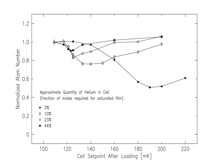
Figure 6: Relative number of atoms trapped as a function of the cell setpoint temperature following accumulation with different helium film thicknesses. For the warmer points, the setpoint was reached within a few seconds and maintained until 30 s after the end of accumulation. For the coldest points, the setpoint was not reached until the latter part of the 30 s post-accumulation period. Since the bolometer sensitivity was different for each film thickness, each curve has been normalized to the lowest temperature point.

5 Trap Loading: Conclusion

The constancy of the number of atoms loaded is probably the most remarkable feature of the trap loading process. The saturation number does not change for wide variations in the film thickness, discharge parameters, cell temperature, and the nature of the conduit between discharge and magnetic trap. Our studies have enabled us to rule out a number of possible loss mechanisms as the limiting factor in loading. A phenomenological model involving a loss term proportional to discharge flux is consistent with our observations, but a physical model remains elusive. Although several aspects of loading are now better understood, we still do not know what process causes the atom number to saturate. To trap more atoms, it may be necessary to increase the effective trap volume, which will require a new magnet system design.

5 UV Laser System

Excitation on the $1S$-$2S$ transition in H requires a powerful, frequency-stable source of 243 nm radiation. In order to achieve the high excitation rates necessary to observe two-body metastable H effects, UV power on the order of 10 mW is required. To sufficiently resolve the Doppler-free spectrum at typical sample temperatures and densities, the UV laser linewidth must be no more than a few kilohertz. With currently available laser technology, these requirements are best satisfied by frequency doubling the output of a 486 nm dye laser which is locked to a stable frequency reference. Following the design of Hänsch and co-workers [54], Sandberg [36] and Cesar [38] developed such a system at MIT; further improvements were introduced by Killian [1]. The remainder of this section describes the UV laser system of the Ultracold Hydrogen Group as used for measurements in this thesis.

1 System Overview

Stable, narrowband light originates in a 486 nm dye laser (Fig. 7), which is a modified Coherent 699 system [55]. The dye solution is circulated at a pressure of 8 bar by a high pressure circulation system purchased from Radiant Dyes [56]. A dye jet of 200 $\mu$m thickness is produced using a polished stainless steel nozzle from the same manufacturer. An intracavity EOM allows for high-bandwidth locking of the laser frequency. When fresh dye solution is pumped by 4 W of violet from a Krypton ion laser, around 650 mW of single-frequency output power is obtained. This power is more than 3 times the specification for an unmodified commercial system.

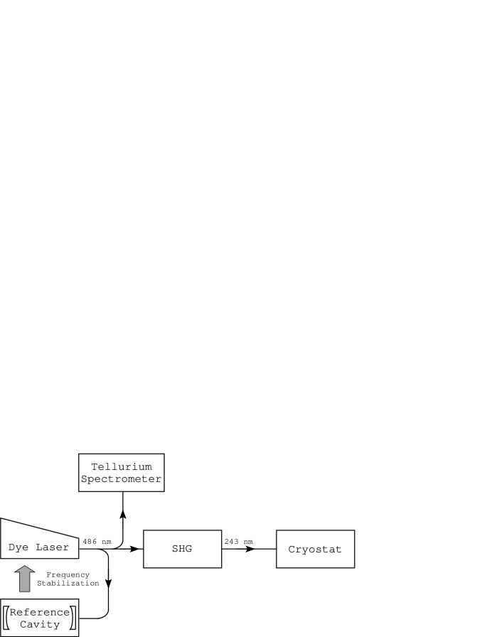
Figure 7: Block diagram of UV laser system.

Frequency stability is achieved by locking the dye laser to a Fabry-Perot reference cavity by the Pound-Drever-Hall phase modulation technique [57]. The cavity, which has a spacer made of zerodur glass, is enclosed in a temperature-stabilized vacuum chamber. It has a free spectral range of 598 MHz and a linewidth of about 600 kHz. When locked to the reference cavity, the laser has a linewidth of about 1 kHz at 486 nm. The reference cavity has a long term drift rate of less than 1 MHz per week.

For finding the cavity resonance closest to the H $1S$-$2S$ frequency, the absorption spectrum of a temperature-stablized Te₂ gas cell serves as an absolute frequency reference. Precise tuning of the laser frequency is achieved by locking the first order diffraction beam from an AOM to the cavity. The AOM drive frequency, which is the offset frequency between laser and cavity, is determined by a high resolution frequency synthesizer. By saturated absorption spectroscopy of a specific Te₂ line [58, 36, 1], the dye laser can be tuned to within several hundred kilohertz of the $1S$-$2S$ frequency.

Most of the 486 nm laser power is coupled into a bow-tie enhancement cavity where the blue light is frequency doubled in a 10 mm long Brewster-cut BBO crystal [36]. The Hänsch-Couillaud [59] scheme is used to lock the cavity in resonance with the incoming blue light. An enhancement factor of $~{}100$ is achieved, resulting in circulating powers as high as 50 W. More than 40 mW of 243 nm light can be generated by this doubling cavity. Due to the large walk-off angle of BBO, the UV is generated in a highly astigmatic transverse mode.

2 UV Beam Transport and Alignment

After passing through astigmatism compensation optics [36], the beam is widened in a telescope for low-divergence propagation to the cryostat, which is 30 m away in a different laboratory. As shown in Fig. 8, the beam passes through another telescope near the cryostat before propagating into the dilution refrigerator. A lens on top of the discharge resonator brings the beam to a focus near the magnetic trap minimum. A concave retromirror glued to the MgF₂ window at the bottom of the trapping cell reflects the beam onto itself, producing the standing wave configuration necessary for Doppler-free two-photon excitation of the $1S$-$2S$ transition.

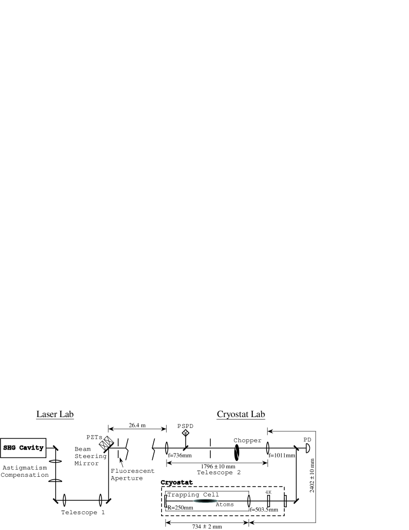
Figure 8: Layout of UV optics in the laser lab, where the UV is generated, and in the cryostat lab, where the atoms are trapped. Several folding mirrors have been omitted, and the drawing is not to scale. The dimensions in the cryostat lab indicate optical path lengths; estimates of thermal contraction have been included in the cryogenic path lengths. A pair of servo circuits tilts the PZT-driven beam steering mirror in the laser lab to fix the beam on a position sensing photodiode (PSPD) in the cryostat lab. A photodiode (PD) monitors the weak beam transmitted from a folding mirror between Telescope 2 and the cryostat. Amplified pulses from this photodiode trigger a timing generator in the data acquisition electronics. In the cryostat, a window thermally anchored at 4 K blocks most of the blackbody radiation from the room-temperature entrance window.

Since the cryostat is located in a different lab, an active beam steering system is required to maintain a steady pointing of the beam into Telescope 2 (see Fig. 8). The beam steering system, which consists of a position sensing photodiode, a servo circuit, and a mirror mounted on piezoelectric transducers (PZT’s), is necessary to compensate for relative motion of the laser table and cryostat and for UV pointing variations due to dye laser pointing instability. The PZT-mounted mirror is 12.7 mm in diameter and 6.4 mm thick. It was mounted using a 5-minute epoxy on a fulcrum and two low voltage PZT stacks [60]; the PZT’s cause deflection in orthogonal directions. We have found this construction to be mechanically robust. In previous incarnations, much thinner (1-2 mm) and lighter mirrors were used to maximize PZT bandwidth. However, the stress on these thin mirrors caused significant distortion of the UV beam at the cryostat. Furthermore, the distortion changed constantly as the PZT voltages required to maintain lock drifted on a time scale of minutes. These problems were eliminated by going to a thicker mirror. The low voltage PZT’s currently in use have very high resonance frequencies. In spite of the relatively large mass of the mirror, a servo bandwidth of several kilohertz is achieved.

To ensure a good overlap of incoming and return beams at the atoms, the position of the return beam is monitored on a fluorescent aperture near the beam steering mirror. The aperture is just large enough to allow the incoming beam to pass through without diffraction effects. While spectroscopy is in progress, the return beam alignment on the aperture is monitored from the cryostat lab via video camera. If the return beam is not centered on the aperture, corrections are made by micromotor translation of one of the Telescope 2 lenses.

The UV beam immediately following the astigmatism compensation optics is nearly square in shape. After propagating nearly 30 m to Telescope 2, the transverse mode consists of a bright central lobe flanked by a series of weaker lobes. The outer lobes are cut off by an iris aperture in Telescope 2. The remaining transverse mode structure is a slightly astigmatic Gaussian beam. By adjusting the length of Telescope 1, more than 60% of the power after Telescope 1 remains after the aperture in Telescope 2. The UV power reaching the atoms is typically 10-20 mW.

In previous spectroscopic experiments with our apparatus, the beam waist near the atoms had a radius of $\sim 50$ $\mu$m. For BEC experiments, it was desirable to employ a tighter focus, since the excitation rate for nearly motionless condensate atoms should scale with the square of laser intensity. It was also desirable to change the size of the waist to study the effects of laser geometry on the $1S$-$2S$ lineshape. For these reasons, the length of Telescope 2 was reduced, resulting in a waist radius of about 21 $\mu$m and a Rayleigh range of 6 mm. These values are calculated by using previously determined Gaussian beam parameters for the input to Telescope 2 and adjusting the length of the telescope for perfect overlap of incoming and return beam modes. In the case of perfect overlap, the position of the waist in the cell is fixed by the radius of curvature of the retromirror. If there is a small mismatch between incoming and return modes, then the incoming and return waists are slightly separated on the trap axis, with the midpoint between waists located at the waist position of ideal overlap. To optimize overlap, the spot sizes of the incoming and return beams are viewed on a folding mirror in Telescope 2, and the length of the telescope is adjusted until they are the same.

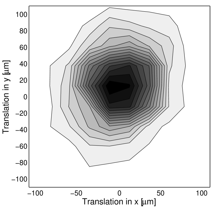
Figure 9: “Lateral scan” image of a trapped hydrogen gas. The number of fluorescence counts is recorded while translating the atoms in a raster pattern with respect to the laser beam. The laser frequency is detuned to the red such that atoms from the central, densest part of the sample (where the cold-collision shift is largest) are excited preferentially. In this example, the sample is slightly offset from the center of the scan range.

Good alignment of the laser beam with the center of the atom cloud is essential for high signal rates and reproducible results. An effective method was developed for achieving this alignment. In our magnet system, there are four “racetrack” quadrupole coils which give rise to the radial confining field of the trap. By adding a small trim current to one coil in each pair of opposing quadrupole coils, it is possible to precisely displace the trap minimum in both directions perpendicular to the trap axis. By placing the trim current in both coils under computer control, it is possible to move the atom cloud rapidly in a lateral raster pattern while exciting the atoms at a constant laser frequency. The resulting plot of excitation signal as a function of trim currents is a kind of spatial image of the atom cloud (Fig. 9). From such a “lateral scan” image, the trim currents can be chosen which center the atom cloud on the laser beam. In addition, if the laser beam axis intersects the trap axis at a significant angle, a highly elliptical distribution results; the lateral scan is a useful diagnostic for overlapping the laser and trap axes.

6 Data Acquisition

1 Lyman-$\alpha$ Detection

The metastables excited in our trap are detected by applying an electric field of about 10 V/cm, which quenches them within a few microseconds. The detection efficiency for the resulting Lyman-$\alpha$ photons is small, however. Due to the closed geometry of the magnet system, the MCP detector sits beyond the lower end of the trapping cell, about 30 cm from the center of the atom cloud. The detection solid angle is only $1.1\times 10^{-2}$ sr. Lyman-$\alpha$ photons must pass through not only the MgF₂ window at the end of the cell but also a second window on the MCP vacuum chamber. Each window transmits at most 40% at 122 nm. The best case quantum efficiency for the MCP itself is about 25%. An upper limit for metastable detection efficiency $\epsilon$ is thus $5\times 10^{-5}$. From measurements described in Ch. 4, $\epsilon$ appears to be about $2\times 10^{-6}$. Most of the additional losses are likely due to absorption on window surfaces and sub-optimal MCP quantum efficiency. Futhermore, at typical $1S$ densities up to 30% of the Lyman-$\alpha$ fluorescence in the detection solid angle is scattered into other directions before it can escape the sample. A discussion of this radiation trapping effect will be presented in Sec. 6.

2 Microchannel Plate Detector

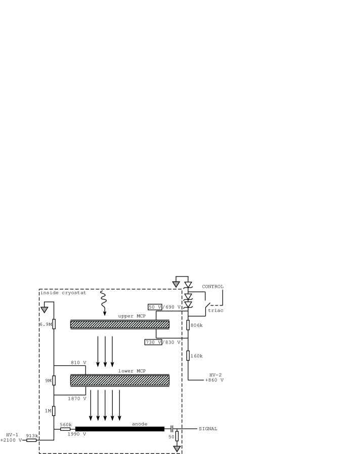
Figure 10: Schematic of MCP switching and biasing circuits. A Lyman-$\alpha$ photon incident on the upper MCP gives rise to a shower of electrons which is further amplified by the lower MCP. The boxed (unboxed) voltage values on the upper MCP correspond to the on (off) state of the detector, controlled by a high voltage triac switch. Room temperature values are given for the resistances and voltages; these may differ by a few percent at low temperature. With HV-1 at 2100 V, significant heating of the MCP occurs on a time scale of minutes. To minimize blackbody heating of the trapping cell, HV-1 is turned on just before the laser excitation phase of the trap cycle and turned off afterwards.

The microchannel plates in the current detector are similar to those described by Killian [1]. In previous work, a Lyman-$\alpha$ filter was used to prevent the detector from being saturated by scatter from the 243 nm laser. The transmission of the filter at 122 nm was only 10%, however. To increase the signal detection efficiency by a factor of 4, the Lyman-$\alpha$ filter was replaced by a MgF₂ window, and a switching scheme was developed which turns on the gain of the upper MCP plate only long enough to detect the Lyman-$\alpha$ fluorescence at each quench pulse.

The relevant circuit diagrams are given in Fig. 10. A triac switch, whose state is governed by a digital signal, allows the voltage across the upper plate to be switched between 140 V and 680 V in a few microseconds. At 140 V the detector is blind to incoming radiation. At 680 V on the upper plate and with the detector biased as shown in Fig. 10, the detector gain is $\sim 10^{6}$. In the present scheme, the channels of the upper plate have a 40:1 length to diameter ratio and the lower plate a 60:1 ratio.

3 Data Acquisition Electronics

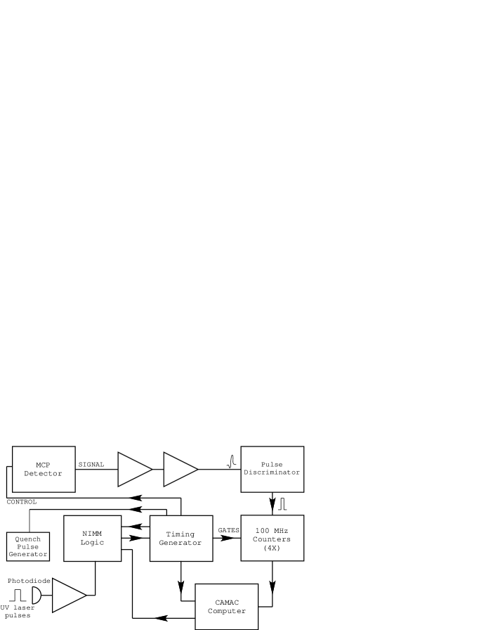
Figure 11: Block diagram of data acquisition electronics used during the laser excitation phase of the trap cycle. Not shown are the rf frequency synthesizers used to tune the laser, drive the rf evaporation coils, and drive the discharge. The synthesizers are controlled by the CAMAC computer via GPIB. The same CAMAC computer also controls an array of A/D and D/A converters for control and monitoring of magnet currents, rf switches, the MCP HV-1 supply, cell temperature, and other diagnostics.

An overview of the data acquisition system is given in Fig. 11. The sequence of events during a trap cycle is determined by a program running on a CAMAC crate computer. When the laser excitation phase begins, a mechanical shutter near the cryostat entrance window opens, and laser pulses are allowed to trigger a timing generator with 8 output channels and sub-microsecond resolution. The timing generator allows precise timing control of the MCP switch and quench (electric field) pulses with respect to the excitation pulses. It also gates four counters to count MCP pulses when signal is present. When the timing generator sequence is finished, the CAMAC computer reads out the counters, the counters are reset, and the timing generator waits to be triggered by the next laser pulse.

4 Metastable Decay Measurements

Figure 12 shows the timing sequence used for the decay measurements described in Ch. 3. The sequence determines wait times for quench pulses following four consecutive laser pulses. Each quench pulse lasts for 90 $\mu$s, and a counter is gated on for the first 40 $\mu$s of each. The MCP is switched on 1.4 ms before each quench in order to fully charge the plates. To obtain more time points in a single decay measurement, a delay generator is enabled before every other trigger, introducing an additional delay between the laser pulse and the start of the timing sequence. For example, the sequence shown in Fig. 12 contains wait times of 2, 11, 38, and 74 ms (not in this order) after the end of a laser pulse; with an additional delay of 18 ms before every other trigger, eight consecutive laser pulses are associated with wait times of 2, 11, 20, 29, 38, 56, 74, and 92 ms. The accuracy of these delay times is limited by phase jitter in the mechanical chopper used to pulse the laser. In the worst case, this jitter leads to a 0.4 ms wait time inaccuracy.

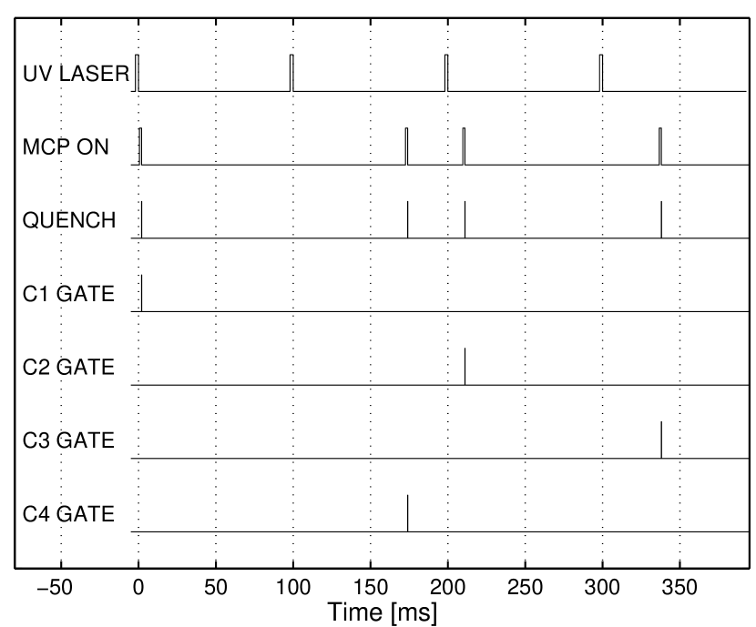
Figure 12: Example timing sequence for a single trigger of the timing generator. C1-C4 indicate counters 1-4. The time axis is referenced to the end of the laser pulse. In this example, triggering occurs with the rise of the first laser pulse at -2 ms. As explained in the text, an additional delay is introduced before every other trigger, resulting in eight different wait times for eight consecutive laser pulses.

Results from a single eight-point decay measurement are shown in Fig. 13. The laser detuning is constant to assure the same metastable density at the beginning of each decay, and the ground state density does not change appreciably during the 800 ms required to make the measurement. The nonstatistical scatter, which arises from fluctuations in laser alignment and power, is typical for a single measurement. To reduce this scatter, many decay curves made at similar laser detuning and $1S$ density are averaged together. As will be explained further in Chapters 3 and 4, the decay curves are analyzed by fitting them with either a simple exponential or a model including both one-body and two-body decay terms.

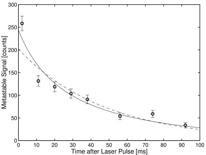
Figure 13: A single metastable decay measurement from a $\sim 100$ $\mu$K sample, recorded with eight laser pulses over 800 ms. The solid line results from fitting with a model including two-body decay, while the dashed line is the best fitting simple exponential.

In the example of Fig. 13, the raw data has been corrected for laser-induced background fluorescence, which has its own characteristic decay behavior (Fig. 14). Although the MCP is $10^{4}$ times less sensitive to 243 nm than to Lyman-$\alpha$, fluorescence photons at 243 nm and longer wavelengths are so numerous after each laser pulse that a few give rise to MCP pulses. The background fluorescence decay is measured at the end of each trap cycle by detuning the laser far off resonance and recording decay curves in the manner described above. The fluorescence decay can be fit to the sum of a fast exponential component and a very long-lived component well approximated by a constant over 100 ms. This fit is used to subtract the background contribution from individual decay curves. For most data, however, the background correction results in only small changes to the metastable decay curves.

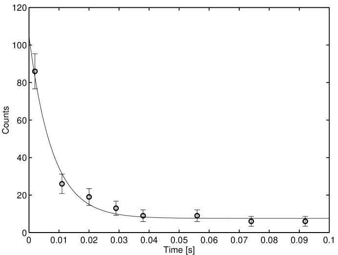
Figure 14: Decay of background fluoresence after a laser pulse. The data here is the sum of 50 decay curves taken with the laser off resonance. The decay is adequately described by the sum of an exponential decay and a constant.

5 Stray Field Compensation

In the presence of an electric field of strength $E$, metastable H quenches at a rate

$$\gamma_{s}=2800E^{2}({\rm cm}^{2}/{\rm V}^{2}){\rm s}^{-1}$$ (11)

due to Stark-mixing with the $2P$ state [61]. To minimize the stray field in our apparatus, we apply a compensation dc offset voltage across the copper film electrodes used for detection quench pulses (Fig. 15(a)). The total electric field ${\bf E}_{\rm tot}$ experienced by the atoms is the sum of applied and stray fields:

$${\bf E}_{\rm tot}={\bf E}_{a}+{\bf E}_{s}.$$ (12)

At any given point in space, the rate $\gamma_{s}$ is proportional to

$$E_{\rm tot}^{2}=(E_{a}+E_{\|})^{2}+E_{\bot}^{2},$$ (13)

where $E_{\|}$ and $E_{\bot}$ are, respectively, the stray field components perpendicular and parallel to the applied field. If both the applied field and the stray field are nearly uniform over the atom cloud, then the optimal compensation voltage is the one which gives $E_{a}=-E_{\|}$. In a situation where only one-body loss mechanisms are important, the total decay rate is the sum of $\gamma_{s}$, the natural decay rate of 8.2 s^-1, and any other one-body rates which may be present. One-body loss dominates in metastable clouds excited from warm, low-density samples. In this case, Eqs. 11 and 13 imply a parabolic dependence of the total decay rate on $E_{a}$, as shown in Fig. 15(b). The best compensation voltage is determined by fitting a parabola to the one-body decay rates measured at several dc voltages. The minimum of the parabola has been found to be stable over several hours.

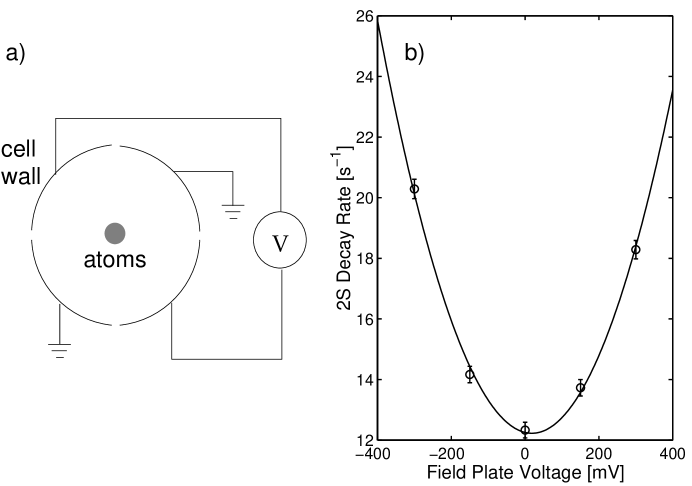
Figure 15: (a) Schematic of trapping cell in cross section, showing electrical connections for the copper film electrodes used for both quench pulses and stray field compensation. (b) Decay rate measurements for different dc electric fields in a single trapped sample. The expected parabolic dependence is observed.

In the current apparatus, two of the electrodes are hard-wired to the electrical ground of the cryostat. This means that stray field compensation is only possible along one direction, and there is a residual stray field with magnitude $E_{\bot}$. An upper limit for the decay rate due to $E_{\bot}$ is 4 s^-1, obtained by subtracting the natural decay rate from the rate at the parabola minimum. This implies that the residual stray field is less than 40 mV/cm.

In future experiments, it should be possible to float all four electrodes, allowing compensation in two dimensions. The stray field component in the third dimension, along the cell axis, is probably very small.

Chapter 2 Trapped Metastable Hydrogen

The physics of metastable hydrogen excited in a magnetic trap is potentially very rich. Metastable H can participate in several types of inelastic collisions, including ones that result in energetic ions. Diffusion is also important. Due to the presence of the $1S$ background gas, a metastable cloud does not immediately fill the volume of the ground state sample, but instead diffuses slowly outward from a region defined by the focus of the excitation laser. In addition, the intense UV radiation can subsequently photoionize many of the metastables.

This chapter summarizes some of the microscopic and macroscopic physics relevant to metastable H in a trap. An understanding of this physics is important for both the interpretation of metastable decay measurements described in Ch. 4 as well as the preparation for future high resolution spectroscopy measurements.

1 Collisions between Metastables

Stimulated by our experimental work, theoretical investigations of $2S$-$2S$ collisions were begun recently. Jonsell et al. have calculated the complex interaction potentials between two metastable hydrogen atoms [62]. Forrey et al. used the potentials to compute elastic, double excitation transfer, and total ionization cross sections [9]. The initial calculations neglected the Lamb shift and fine structure, and the results were considered valid for thermal energies large compared to the splittings between $2S_{1/2}$, $2P_{1/2}$, and $2P_{3/2}$ states (that is, for $T\gg 1$ K). In the past year, Forrey, Jonsell, and collaborators have included the Lamb shift and fine structure in their potentials, allowing the first calculations of elastic and inelastic $2S$-$2S$ rate constants down to $T=0$ [7]. The effect of the hyperfine interaction has not yet been included, but the rate calculations which neglect hyperfine structure are expected to be accurate to within an order of magnitude [63].

As described in Ch. Studies with Ultracold Metastable Hydrogen, the trapped metastables are in the $d$ state $(F=1,m_{F}=1)$ of the $2S$ manifold. Just as with the $1S$ $d$-state atoms, dipolar decay collisions can change the hyperfine state of the metastables, causing them to be lost from the trap. The rate constants for the inelastic $d+d$ channels of the $2S$ manifold have not been calculated. However, the approach of Stoof, et al. for $1S$ dipolar decay collisions [40] is applicable to the $2S$ case as well. The rate for $2S$ dipolar decay is governed by weak magnetic dipole interactions between atoms. These interactions in the $2S$-$2S$ case are similar in strength to the $1S$-$1S$ case, and the corresponding inelastic rates are not expected to differ by more than an order of magnitude [49]. At the metastable densities achieved in the experiments described in Ch. 4, $2S$ dipolar decay should be undetectable.

Several $2S$-$2S$ collision processes which may occur in the trap are outlined below in more detail. Unless denoted otherwise, the label “$2S$” refers to the magnetically trapped $d$ state of the $2S$ manifold.

1 Summary of $2S$-$2S$ Collision Processes

Elastic Collisions.

$$H(2S)+H(2S)\longrightarrow H(2S)+H(2S).$$ (1)

According to recent theoretical calculations [7], these collisions occur more frequently than $2S$-$2S$ inelastic collisions at all temperatures accessible in our trap. However, due to the fact that the metastable density is several orders of magnitude smaller than the ground state density, elastic $2S$-$2S$ collisions are much less frequent than elastic $1S$-$2S$ collisions. They contribute insignificantly to the dynamics of the metastable cloud, and they are not detectable in current experiments.

Excitation Transfer. During a collision between metastables, either one or both of the atoms may undergo a transition to the $2P$ state. The processes are formally known as single excitation transfer,

$$H(2S)+H(2S)\longrightarrow H(2P)+H(2S),$$ (2)

and double excitation transfer,

$$H(2S)+H(2S)\longrightarrow H(2P)+H(2P).$$ (3)

These collisions are, in principle, directly detectable because the $2P$ products radiate Lyman-$\alpha$ after a lifetime of 1.6 ns. At high temperatures, where the $2S$ and $2P$ levels can be considered degenerate, the allowed molecular symmetries for a pair of metastables do not permit single excitation transfer [9]. Single excitation transfer may be allowed at low temperatures, but it would require coupling between the orbital angular momentum of the nuclei and the electronic angular momentum. The calculations of Forrey, et al. to date have assumed that this coupling is zero. Forthcoming theoretical work will determine whether this assumption is justified for spin-polarized metastables [63].

The rate constant for excitation transfer collisions is predicted to be larger than the rate constant for ionizing collisions at all temperatures.

Ionization. Two types of ionization can occur when metastables collide. One type is Penning ionization,

$$H(2S)+H(2S)\longrightarrow H(1S)+H^{+}+e^{-},$$ (4)

which liberates 6.8 eV ($7.9\times 10^{4}$ K) of energy. Most of the energy is imparted to the electron, which leaves the trap instantly. A fraction of the energy approximately equal to $m_{e}/m_{p}$, the electron-to-proton mass ratio, becomes the kinetic energy associated with the center of mass of the H ion (proton) and ground state atom. This small fraction still amounts to more than 40 K, and the proton and atom will generally leave the trapped sample within a couple microseconds. The magnetic field at the center of the trap is far too weak to hold the proton in a cyclotron orbit; the proton will quickly move away from the trap axis and towards the cell wall, guided by the radially-pointing magnetic field of the quadrupole magnets.

The second type of ionization is associative,

$$H(2S)+H(2S)\longrightarrow H_{2}^{+}+e^{-}.$$ (5)

Between 6.8 eV and 9.45 eV of translational energy is liberated, depending on the rovibrational state of the molecular ion. By arguments similar to those of the preceding paragraph, both the ion and electron products leave the trap quickly.

The cross section for associative ionization has been measured in beam experiments for collision energies down to 4.1 meV (48 K) [6]. At this energy, the measured cross section for associative ionization is 100 times smaller than the theoretical total ionization cross section [9], indicating that Penning ionization is far more prevalent than associative ionization. The experiments showed that the associative cross section varied as $E^{-1}$ at high temperatures, while theory predicts the total ionization cross section to vary as $E^{-2/3}$. It has not yet been established whether Penning ionization also dominates at low temperatures.

Dipolar Decay. Due to the electron-electron and electron-proton magnetic dipole interactions between two $2S$ atoms, inelastic collisions can occur in which the sum of magnetic quantum numbers $m_{F}$ of the two atoms is not conserved. The hyperfine state of one or both atoms can change from $d$ to another hyperfine state which is weakly-trapped or anti-trapped. Under typical trap conditions, enough kinetic energy is liberated in the transition to eject even the weakly-trapped products from the trap. Very generally, these dipolar decay transitions can be written

$$H(2S,d)+H(2S,d)\longrightarrow H(2S,\mu)+H(2S,\nu),$$ (6)

where at least one of $\mu$ and $\nu$ is not $d$. These magnetic interactions are weak compared to the central forces responsible for other inelastic processes. For ground state H, the sum of rate constants for dipolar decay of $d$ states was determined to be $\sim 10^{-15}$ cm³/s across the range of temperatures and magnetic fields relevant to hydrogen trapping [40, 64]. The same order of magnitude is expected for the sum of rates corresponding to Eq. 6.

2 Theoretical Rate Constants

The rate constants for double excitation transfer and ionizing $2S$-$2S$ collisions have recently been calculated down to $T=0$ and are summarized in Fig. 1. The methods of calculation are outlined in [9] and a forthcoming paper [7]. For each collision channel $i$, the corresponding rate constant $R_{i}$ is defined such that $R_{i}n_{2S}^{2}$, where $n_{2S}$ is the local density of metastables, is the local rate of collision events of type $i$. If we assume that double excitation transfer and ionization are much more prevalent than other inelastic collisions, the total two-body loss constant $K_{2}$ can be expressed

$$K_{2}=2(R_{\rm et}+R_{\rm ion}),$$ (7)

where $R_{\rm et}$ and $R_{\rm ion}$ are the rates for double excitation transfer and ionization. The factor of 2 appears since two metastable atoms are lost from the trap in each collision event. Chapter 4 describes how $K_{2}$ was determined experimentally.

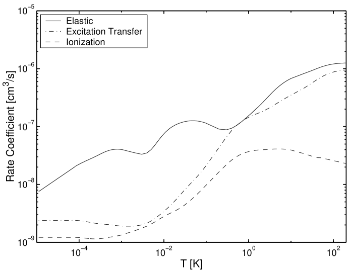
Figure 1: Theoretical rate constants for $2S$-$2S$ collisions as a function of temperature, courtesy of Forrey, et al. 

As can be seen from Fig. 1, below $10^{-4}$ K the elastic collision rate varies as $T^{1/2}$, and the inelastic rates are nearly independent of temperature. In this regime, only $s$-wave collisions are important, and both the elastic and inelastic collisional behavior of metastable H are characterized by a single quantity, the complex scattering length $a_{2S-2S}$. In general, for a complex $s$-wave scattering length $a=\alpha-i\beta$ involving identical bosons, the elastic cross section is given by

$$\sigma_{\rm el}=8\pi(\alpha^{2}+\beta^{2}),$$ (8)

and the inelastic cross section by

$$\sigma_{\rm inel}=8\pi\beta/k,$$ (9)

where k is the relative wave vector of the colliding atoms [10]. The elastic cross section at collision energy $kT$ is thus independent of $T$ while the inelastic cross section has a $1/k\sim T^{-1/2}$ dependence. This $1/k$ dependence of $\sigma_{\rm inel}$ is an example of the Wigner threshold law [65, 66]. To find the rate constants for a thermal sample, the average over a Maxwell-Boltzmann distribution is taken: $R_{i}=\langle\sigma_{i}v\rangle$. The resulting elastic rate goes as $T^{1/2}$, and the inelastic rate is given by $R_{\rm inel}=8\pi\hbar\beta/\mu$, where $\mu$ is the two-body reduced mass. The results of Forrey and co-workers [7] imply that in the zero temperature limit

$$a_{2S-2S}=\alpha-i(\beta_{\rm et}+\beta_{\rm ion}),$$ (10)

where $\alpha=20.4$ nm, $\beta_{\rm et}=0.75$ nm, and $\beta_{\rm ion}=0.38$ nm.

Since metastable hydrogen can be excited at temperatures below 100 $\mu$K, our experiments are able to probe the theoretically predicted Wigner threshold regime. It should be noted, however, that even up to temperatures as high as 10 mK, the theoretical inelastic collision rates do not change by more than a factor of 2.

The accuracy of the theoretical rates is difficult to estimate. Hyperfine structure has not yet been included in the calculations, nor an allowance for coupling between electronic angular momentum and nuclear orbital angular momentum. In addition, the effects of the trapping magnetic field on the collision rates have not been examined. For the magnetic fields of a few gauss experienced by colder samples, the rate constants are predicted to be accurate to within an order of magnitude.

2 Collisions between Metastable and Ground State Atoms

In our experiments, the peak metastable densities are typically three or more orders of magnitude smaller than the peak ground state density. Although the $1S$-$2S$ cross sections are smaller than the $2S$-$2S$ cross sections, the metastables still collide with ground state atoms much more frequently than with each other. Most of the $1S$-$2S$ collisions are elastic, and most of what has been learned theoretically and experimentally about $1S$-$2S$ interactions so far pertains to elastic collisions.

1 Elastic $1S$-$2S$ Collisions

With the advent of ab initio calculations for the short range $1S$-$2S$ molecular potentials, it became possible in the last decade for theorists to predict $a_{1S-2S}$, the $s$-wave elastic scattering length. Since $1S$-$2S$ collisions are predominantly $s$-wave at the temperatures of magnetically trapped hydrogen, this single parameter is sufficient to describe the elastic collisions. The elastic cross section, $\sigma_{1S-2S}=4\pi a_{1S-2S}^{2}$, is independent of collision energy.

Calculations of $a_{1S-2S}$ depend sensitively on the molecular potential. A first calculation of $a_{1S-2S}$ was made by Jamieson, et al. [3] using the best available ab initio potential of the time, which extended only to 20 bohr. The result was $a_{1S-2S}=-2.3$ nm. The accuracy of this calculation was limited by (1) the mismatch between the short range potential and the asymptotic long range potential and (2) uncertainty in the very short range part of the ab initio potential. More recently, Orlikowski and collaborators recalculated the entire short range potential, extending it to 44 bohr and realizing a much better match to the long range potential [4]. From their improved potential, they found $a_{1S-2S}=-3.0$ nm. Although the uncertainty is difficult to estimate [67], this is believed the most accurate calculation of $a_{1S-2S}$ to date.

As mentioned in Ch. Studies with Ultracold Metastable Hydrogen, there is a density-dependent cold-collision shift of the $1S$-$2S$ transition frequency due to the difference in $1S$-$2S$ and $1S$-$1S$ interactions. Since the $1S$-$1S$ scattering length is theoretically known to be $a_{1S-1S}=0.0648$ nm with a relatively small uncertainty [68], the cold-collision shift parameter $\chi=\Delta E_{1S-2S}/hn_{1S}$ can be used to measure $a_{1S-2S}$ provided that the relationship between the shift and scattering lengths is well understood. According to the arguments given by Killian [1], the energy shift of the $1S$-$2S$ transition for homogeneous weak excitation in a homogeneous ground state gas of density $n_{1S}$ is

$$\Delta E_{1S-2S}=\frac{8\pi\hbar^{2}n_{1S}}{m}(a_{1S-2S}-a_{1S-1S}),$$ (11)

where $m$ is the atomic mass. The fact that the two scattering lengths in this formula are multiplied by the same factor follows from assuming uniform coherent excitation of the many-body wave function of the ground state gas. The bosonic bunching correlations which enhance the $1S$-$1S$ interactions are maintained as each $1S$ atom in the many-body wave function gains $2S$ character. Eq. 11 has been derived by Stoof and Pethick using a microscopic approach [5], and a more general sum rule extension of Eq. 11 to inhomogeneous cases has recently been posited by Oktel and collaborators [69]. If instead we consider the case where a $2S$ atom is introduced into a homogeneous $1S$ gas by means other than coherent excitation, then Hartree-Fock theory predicts that the energy of the $2S$ state will be shifted only half as much; this is because $1S$ and $2S$ atoms are distinguishable particles and, in this case, they are spatially uncorrelated. The energy difference between the two states would then be

$$\Delta E_{1S-2S}=\frac{4\pi\hbar^{2}n_{1S}}{m}(a_{1S-2S}-2a_{1S-1S}).$$ (12)

Both Eq. 11 and Eq. 12 assume that the contributions of inelastic processes to the energy shifts are negligible.

The MIT Ultracold Hydrogen Group used Eq. 11 to determine $a_{1S-2S}=-1.4\pm 0.3$ nm from the experimental cold-collision shift [2], which is a factor of two smaller than the value of Orlikowski, et al.  Interestingly, if Eq. 12 is used, $a_{1S-2S}=-2.9\pm 0.6$ nm is obtained, in good agreement with the theoretical value. This suggests that Eq. 12 is closer to the correct description of the cold-collision shift in our experiment. Further support for this conclusion is provided by recent time-resolved spectroscopic measurements of hydrogen BEC’s performed in our group [43, 70]. A possible reason why Eq. 12 may be favored over Eq. 11 is that $1S$-$2S$ collisions occurring during the excitation may destroy the spatial correlations of the ground state gas. Furthermore, it remains an open question how to correctly describe the cold-collision shift in terms of scattering lengths for the experimentally realistic case of an inhomogeneous thermal gas and an inhomogeneous laser field.

In the remainder of this thesis, the theoretical value of $a_{1S-2S}$ will be assumed correct. This implies an elastic scattering cross section $\sigma_{1S-2S}=1.1\times 10^{-12}$ cm². The magnitude of $\sigma_{1S-2S}$ is important for determining the rate at which metastables can diffuse through the ground state sample.

2 Inelastic $1S$-$2S$ Collisions

At least two types of inelastic collisions are possible between metastables and ground state H in the trap. First, there is the analog of dipolar decay,

$$H(1S,d)+H(2S,d)\longrightarrow H(1S,\mu)+H(2S,\nu),$$ (13)

where at least one of the products is not a $d$-state. As mentioned in Sec. 1, these processes are mediated by weak magnetic dipole forces, and their rates should be small compared to the important $2S$-$2S$ inelastic channels. Second, excitation transfer can occur as follows:

$$H(1S)+H(2S)\longrightarrow H(1S)+H(2P).$$ (14)

To our knowledge, no theoretical work has been done to date on inelastic $1S$-$2S$ collisions. If they occur at significant rates in the hydrogen trap, then they should be observable as one-body metastable decay processes; the decay component would be a simple exponential since the ground state density does not change appreciably during the metastable lifetime. An upper limit for these rates based on decay measurements is presented in Ch. 4.

3 Photoionization

The 243 nm UV photons which create metastable H can also ionize the metastables (Fig. 2). By cubic interpolation of the tabulated values from Burgess [71], the cross section for photoionization is found to be $\sigma_{\rm pi}=6.2\times 10^{-18}$ cm² at 243 nm. If we express the single-atom photoionization rate due to incident laser intensity $I$ as $\alpha_{\rm pi}I$, the proportionality constant is $\alpha_{\rm pi}=7.6\times 10^{-3}$ (mW/cm²)^-1s^-1.

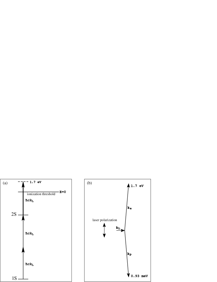
Figure 2: (a) Energy level diagram for excitation and photoionization of metastable hydrogen with a 243 nm laser. The energy $\hbar ck_{L}$ of each photon is 5.1 eV. (b) Momentum diagram in the lab frame for photoionization of a trapped metastable H atom. In the center-of-mass frame of the atom, the most probable direction of electron emission is along the laser polarization. The size of ${\bf k}_{L}$ in proportion to the electron wavevector ${\bf k}_{e}$ and proton wavevector ${\bf k}_{p}$ has been exaggerated in this diagram.

At warmer sample temperatures ($>1$ mK), the volume of the metastable cloud which forms during the laser pulse is much larger than the laser beam, and the fraction of atoms experiencing high laser intensity at any given time is small. As a consequence, only a small fraction of the metastables are photoionized. In colder samples, however, a significant fraction of the metastables are in the laser field. For samples below 100 $\mu$K, photoionization may be the most important metastable loss process during the excitation pulse.

For a given trap shape, temperature, sample density, and laser intensity distribution, we can numerically calculate the fraction of metastables $\mathcal{F}_{\rm pi}$ which are lost to photoionization during an excitation pulse. This calculation is straightforward assuming that the time required to establish a quasi-static metastable spatial distribution $f_{2S}({\bf r})=f_{2S}(\rho,z)$ is short compared to the length of the excitation pulse. Since the collision time and radial transit time are both typically 10 times or more shorter than the pulse length at $\sim 100$ $\mu$K, this is a good assumption for colder samples (see Sec. 4).

To find $\mathcal{F}_{\rm pi}$, we consider the number of atoms $N_{z,2S}(z,t)$ in a slice perpendicular to the trap axis at $z$ with thickness $dz$. In each slice,

$$\dot{N}_{z,2S}(z,t)=R_{12}(z)-\Phi(z)N_{z,2S}(z,t),$$ (15)

where $R_{12}(z)$ is the total rate of metastable generation due to laser excitation, and $\Phi(z)$ is the fraction of metastables which are photoionized per unit time. The distribution $R_{12}(z)$ can be calculated using the Monte Carlo simulation of excitation described in Sec. 3. If $t=0$ corresponds to the beginning of the excitation pulse, the solution to Eq. 15 for times up to the end of the pulse can be written

$$N_{z,2S}(z,t)=R_{12}(z)C(z,t)t,$$ (16)

where $C(z,t)$ is a correction factor which expresses the effect of photoionization on the otherwise linear growth of the metastable population at $z$. The time-dependent correction factor is given by

$$C(z,t)=\frac{1}{\Phi(z)t}\left(1-e^{-\Phi(z)t}\right).$$ (17)

The fraction photoionized at $z$ per unit time is found by evaluating

$$\Phi(z)=\frac{\alpha_{\rm pi}\int d\rho\ \rho f_{2S}(\rho,z)I_{\rm tot}(\rho,z)}{\int d\rho\ \rho f_{2S}(\rho,z)},$$ (18)

where $I_{\rm tot}$ is the sum of incoming and return laser beam intensities. The fraction of metastables photoionized in a pulse of length $t$ is the spatial average of $C(z,t)$:

$$\mathcal{F}_{\rm pi}(t)=\frac{\int f_{2S}({\bf r})C(z,t)\,d^{3}{\bf r}}{\int f_{2S}({\bf r})\,d^{3}{\bf r}}.$$ (19)

As an example, for perfectly overlapped UV beams in the 87 $\mu$K sample of Trap W in Ch. 3, the fraction of $2S$ atoms lost to photoionization during a 2 ms excitation pulse is found to be $\mathcal{F}_{\rm pi}=0.28$ at 12 mW of UV power and $\mathcal{F}_{\rm pi}=0.38$ at 18 mW. The fraction photionized has a weak dependence on the beam radius, the laser detuning, and the location of the laser focus along the trap axis.

At $T\sim 100~{}\mu$K the rate of metastable production in the trap should begin to saturate due to photoionization after a few milliseconds. This expectation was confirmed in a preliminary experiment which recorded signal rates in consecutive trap cycles using different pulse lengths (see Fig. 2).

A natural question to ask is whether any of the charged particles generated by photoionization remain in the trap long enough to affect the metastable cloud. If enough space charge lingers after a laser pulse, the metastables could quench in the resulting electric field. To investigate this, we consider the energy and momentum of the resulting proton-electron pair (see Fig. 2). Almost all of the of energy above threshold, 1.7 eV ($2.0\times 10^{4}$ K), goes to the electron, causing the electron to leave the trap instantaneously. The proton recoils with a fraction $m_{e}/m_{p}$ of the electron energy, about 0.93 meV (11 K). In the center-of-mass frame, this recoil is opposite to the direction of electron emission. For an $S$-orbital electron, the angular distribution of photoelectric emission is peaked around the laser polarization axis (see [72], for example). The lab frame does not look much different from the center-of-mass frame, since the initial momenta of the photon and atom are small compared to the photoionization momentum. In our experiments, the excitation laser is linearly polarized in a direction perpendicular to the trap axis; this means that the protons will recoil in a radial direction, exiting the atom cloud in less than 1 $\mu$s. Similar to the case of ion collision products described in Sec. 1, the protons quickly move into the quadrupole field, where the magnetic field is parallel to the direction of motion. In this way, the protons leave the trap without causing much loss in the sample.

4 Dynamics of the Metastable Cloud

The dynamics of the $2S$ cloud are more complex than the dynamics of the quasi-equilibrium $1S$ cloud. This is because the metastables are excited at the focus of the laser and spread along the trap axis by diffusion. At the densities typical of experiments described in this thesis, the lifetime of the metastables is much shorter than the time required to establish equilibrium along the axis.

Since Doppler-free excitation imparts no momentum to an atom, each metastable atom initally possesses the velocity of the ground state atom from which it was excited. Different velocity classes in the ground state gas have different probabilities for excitation, however, and it is because $2S$ atoms collide frequently with $1S$ atoms that a Maxwell-Boltzmann velocity distribution is quickly established in the metastable cloud. The $1S$-$2S$ collision time is between 100 $\mu$s and 1 ms for typical sample densities, and an equilibrium velocity distribution is established within a few collision times [73]. Since the mean free path of the $2S$ atoms $l=(\sqrt{2}n_{1S}\sigma_{1S-2S})^{-1}$ is typically comparable to the thermal radius of the $1S$ cloud (0.7 mm at 2.5 mK, 0.18 mm at 100 $\mu$K), an equilibrium radial spatial distribution is achieved on a short time scale. In other words, the radial extent of the metastable cloud quickly matches the radial extent of the ground state cloud.

Much more time is required for the metastable cloud to spread out to its equilibrium extent in the axial direction, however. The metastable cloud is excited in a region along the trap axis which is defined by the depth of focus of the laser. Initially, the length of the $2S$ cloud between its 1/e density points is $\sim 2$ cm, while the length of the ground state cloud varies between 4 cm and 24 cm. The distance which $2S$ atoms must travel along $z$ to fill up the equilibrium trap volume is more than 100 times longer than a mean free path. Thus, to approach equilibrium, the metastables must diffuse along the trap axis. The time required is typically much longer than the lifetime of the $2S$ state.

If we neglect for the moment $2S$-$2S$ inelastic collisions, a metastable cloud excited from a ground state sample with peak density of at least a few times 10¹³ cm^-3 will have a quasi-static spatial distribution. This is because (1) the metastable cloud is axially confined by $1S$-$2S$ collisions and (2) radial equilibrium is maintained over the lifetime of the metastable cloud. To examine the transport of the cloud more generally, we must consider the diffusion of $2S$ atoms in a $1S$ background gas.

To accurately describe the time evolution of the metastable distribution, the density-dependent losses due to $2S$-$2S$ inelastic collisions must also be considered. The effects of diffusion and two-body losses on the metastable cloud shape have been studied using a dynamic simulation described in Sec. 3. One of the inputs to this simulation is a parameter describing the rate of diffusion along the trap axis; the remainder of this section summarizes an approach for determining the diffusion parameter.

1 Diffusion Constant

From the results of a hard-sphere kinetic theory, the diffusion constant for a dilute gas of one species in a background gas of another species with the same atomic mass is

$$D=\frac{4}{3\sigma n}\sqrt{\frac{kT}{\pi m}},$$ (20)

where $n$ is the background gas density, $\sigma$ is the cross section for collisions between the two species, and $m$ is the atomic mass [74]. The dilute gas atoms are here assumed to collide much more frequently with the background gas atoms than with each other. For the case of $2S$ atoms in a $1S$ gas, Eq. 20 becomes

$$D=6.1\times 10^{15}\frac{T^{1/2}}{n_{1S}}~{}{\rm cm}^{-1}{\rm s}^{-1}{\rm K}^{-1/2},$$ (21)

where the theoretical value of $\sigma_{1S-2S}$ has been used.

If the length scales for variations in $n_{1S}$ were much larger than the $2S$ mean free path in all directions, then a three-dimensional diffusion equation

$$\frac{\partial n_{2S}}{\partial t}=D\nabla^{2}n_{2S}$$ (22)

would describe the transport of the metastables. However, as mentioned above, an equilibrium distribution is rapidly established in the radial direction. Futhermore, the $2S$ atoms oscillate through the radial density distribution at a frequency comparable to the $1S$-$2S$ collision frequency. A better approach is to find the effective diffusion constant along the trap axis as a function of the peak ground state density. In this way, metastable transport in the trap can be described as a one-dimensional diffusion process.

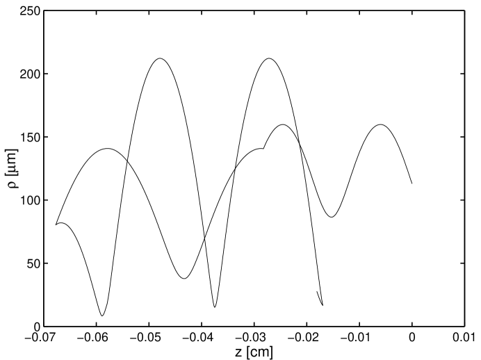
Figure 3: Trajectory of a metastable atom in the $z$-$\rho$ plane over a 2 ms period, generated by Monte Carlo simulation. The trajectory begins at $z=0$, and kinks are evident at the points where momentum-changing collisions with ground state atoms occur. The regular oscillations in $\rho$ are due to quasi-elliptical orbits about the trap axis occurring at a frequency of $\sim 3$ kHz.

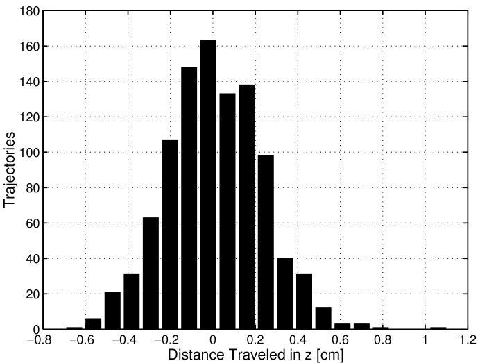
Figure 4: Histogram of net distance traveled in $z$ for 1000 metastable atom trajectories followed over 20 ms. The temperature is 87 $\mu$K, and peak $1S$ density is $5.7\times 10^{13}$ cm^-3. These are close to the peak density conditions of Trap W in Ch. 4.

2 Monte Carlo Diffusion Simulation

The rate of diffusion in $z$ has been studied by Monte Carlo simulation of metastable atom trajectories. The computer simulation uses a normally-distributed random number generator to select the components of an initial $2S$ atom velocity ${\bf v}$ from the Maxwell-Boltzmann distribution. The equations of motion for the atom are integrated in a trap potential $U$ whose shape is specified by the sum of an axial bias field and a radial field gradient. To simplify the coding, the variation of the trapping field in $z$ is neglected. Collisions are simulated by taking time steps $dt$ much shorter than the average collision time and using random numbers to test for a collision in each time step. The collision probability per step is $n_{1S}\sigma_{1S-2S}v~{}dt$, where $n_{1S}=n_{1S,o}e^{-U/kT}$. After each collision, a new random velocity is selected.

Fig. 3 shows an example trajectory calculated in this way. In a typical simulation, 1000 such trajectories are generated, each covering a period of tens of milliseconds. Statistics are collected for the trajectories, including the distribution of distances traveled in $z$ (Fig. 4). The rms width of the distribution, $\sigma_{z}$, serves as a measure of the characteristic diffusion length for the given trap conditions. At a peak $1S$ density $n_{1S,o}=6\times 10^{13}$ cm^-3and $T=90~{}\mu$K (Trap W of Ch. 4), $\sigma_{z}$ is 2.3 mm after a period $t=20$ ms. The $1S$-$2S$ collision rate is found to be about half that expected in a uniform sample at the peak density of the trap.

It was verified that $\sigma_{z}$ is proportional to $t^{1/2}$ and inversely proportional to $n_{1S,o}^{1/2}$, as expected for a diffusion process. The distribution of distances traveled did not depend on the choice of initial $\rho$.

5 Fluorescence in a Quenching Field

For the measurements in this thesis, metastables were detected by applying a quenching electric field and observing the Lyman-$\alpha$ fluorescence. The recoil energy associated with this photon is 670 $\mu$K. Whether or not the recoiling atom leaves the trap depends on the depth of the trap and the ground hyperfine state into which the atom decays. The relevant traps in Ch. 4 are all deeper than the recoil energy for the $\left|1S_{d}\right\rangle$ state, but not for the weakly-trapped $\left|1S_{c}\right\rangle$ state. Generally speaking, atoms returning to the $\left|1S_{d}\right\rangle$ state in these relatively deep traps remain trapped, but atoms returning to other hyperfine states will leave the sample.

To calculate the branching ratios of trapped metastable H in a quenching electric field, it is necessary to know the eigenstate $\left|2S^{\prime}_{d}\right\rangle$ in the presence of simultaneous electric and magnetic fields. Numerical diagonalization of a Hamiltonian including interactions with weak fields E and B reveals that the state is

$$\left|2S^{\prime}_{d}\right\rangle=\left|2S\uparrow\mbox{$\uparrow\!\!\!\!\!\!\!\!\>\>-$}\right\rangle-10^{-3}E\Bigl{[}({\rm cos}\,\gamma)\Bigl{(}1.82\left|\uparrow\>\downarrow\mbox{$\uparrow\!\!\!\!\!\!\!\!\>\>-$}\right\rangle-0.90\left|\rightarrow\>\uparrow\mbox{$\uparrow\!\!\!\!\!\!\!\!\>\>-$}\right\rangle\Bigr{)}+$$

$${}+({\rm sin}\,\gamma)\Bigl{(}1.26\left|\rightarrow\>\downarrow\mbox{$\uparrow\!\!\!\!\!\!\!\!\>\>-$}\right\rangle-1.51\left|\downarrow\>\uparrow\mbox{$\uparrow\!\!\!\!\!\!\!\!\>\>-$}\right\rangle\Bigr{)}\Bigr{]},$$ (23)

where $E$ has units of V/cm, and $\gamma$ is the angle between E and B [36]. The first label in each ket on the right-hand-side of Eq. 23 indicates the orbital state, while the second and third labels indicate the electron and proton spin states, respectively. A shorthand notation has been used for the $2P$ components: $\uparrow$, $\rightarrow$, and $\downarrow$ as a first label denote the orbital states $\left|2\>1\>1\right\rangle$, $\left|2\>1\>0\right\rangle$, and $\left|2\>1\>-\!\!1\right\rangle$ of the $\left|n\>L\>m_{L}\right\rangle$ basis, respectively. The expression is valid provided both the Stark shift and Zeeman shift are small compared to the Lamb shift separating $2S$ and $2P$; the experimental situation is well within this regime. The relative probability of decaying to each of the ground hyperfine states, which in the relevant magnetic field regime are

$$\left|1S_{a}\right\rangle = \frac{1}{\sqrt{2}}\left[\left|1S\downarrow\mbox{$\uparrow\!\!\!\!\!\!\!\!\>\>-$}\right\rangle-\left|1S\uparrow\mbox{$\downarrow\!\!\!\!\!\!\!\!\>\>-$}\right\rangle\right]$$ (24)

$$\left|1S_{b}\right\rangle = \left|1S\downarrow\mbox{$\downarrow\!\!\!\!\!\!\!\!\>\>-$}\right\rangle$$ (25)

$$\left|1S_{c}\right\rangle = \frac{1}{\sqrt{2}}\left[\left|1S\uparrow\mbox{$\downarrow\!\!\!\!\!\!\!\!\>\>-$}\right\rangle+\left|1S\downarrow\mbox{$\uparrow\!\!\!\!\!\!\!\!\>\>-$}\right\rangle\right]$$ (26)

$$\left|1S_{d}\right\rangle = \left|1S\uparrow\mbox{$\uparrow\!\!\!\!\!\!\!\!\>\>-$}\right\rangle,$$ (27)

is obtained from the squares of the dipole matrix elements between these states and $\left|2S^{\prime}_{d}\right\rangle$. For a fixed position in the trap, the fraction of atoms $F_{d}$ returning to $\left|1S_{d}\right\rangle$ is

$$F_{d}=\frac{0.81+2.28\,{\rm tan}^{2}\gamma}{4.12+3.87\,{\rm tan}^{2}\gamma}.$$ (28)

This ratio ranges from 20% when E and B are parallel to 59% when the fields are perpendicular. To find the branching ratio for the sample as a whole, $F_{d}$ must be averaged over the metastable distribution. One way to calculate this average is by a Monte Carlo simulation, described in Sec. 6. It turns out that nearly 50% of the metastables in a typical trap return to $\left|1S_{d}\right\rangle$, subsequently thermalizing with the ground state cloud.

Polarization	Contributing Matrix Elements	Total Probability
	$\left\langle 1S_{d}\left|z\right|2S^{\prime}_{d}\right\rangle$
$\pi$	$\left\langle 1S_{c}\left|z\right|2S^{\prime}_{d}\right\rangle$	$(0.78\,{\rm sin}^{2}\gamma+0.81)/{\mathcal{N}}$
	$\left\langle 1S_{a}\left|z\right|2S^{\prime}_{d}\right\rangle$
$\sigma^{-}$	$\left\langle 1S_{d}\left|x-iy\right|2S^{\prime}_{d}\right\rangle$	$2.28\,{\rm sin}^{2}\gamma/{\mathcal{N}}$
$\sigma^{+}$	$\left\langle 1S_{a}\left|x+iy\right|2S^{\prime}_{d}\right\rangle$	$3.31\,{\rm sin}^{2}\gamma/{\mathcal{N}}$
	$\left\langle 1S_{c}\left|x+iy\right|2S^{\prime}_{d}\right\rangle$

Table 1: Probability of a Lyman-$\alpha$ fluorescence photon having each of the three possible polarizations as a function of $\gamma$, the angle between B and the quenching electric field E at the location of the emitting atom. The probabilities are calculated by summing the squares of the contributing dipole matrix elements. The normalization factor is ${\mathcal{N}}=0.25\,{\rm cos}^{2}\gamma+3.87$.

When examining the effect of sample geometry on the detection efficiency for metastables, it is necessary to consider the polarization of the emitted Lyman-$\alpha$ photons. The polarization of a photon emitted in a transition between specific $2P$ and $1S$ hyperfine states is determined by the change in $m_{L}$ represented in the contributing dipole matrix element. The relative probabilities of obtaining $\pi$, $\sigma^{+}$, and $\sigma^{-}$ polarization as a function of $\gamma$ are summarized in Table 1. The dipole radiation patterns with respect to the orientation of B depend on the polarization (Table 2) [77]. For a quenched metastable, taking into account the probability of emitting into each polarization, the angular probability distribution of fluorescence is shown in Fig. 5 for the limiting cases of $\gamma=\pi/2$ and $\gamma=0$. In the lab frame, the far-field angular distribution can be obtained by taking a spatial average over the local emission patterns in the metastable cloud.

Polarization	Angular Distribution
$\pi$	$\frac{3}{8\pi}\,{\rm sin}^{2}\beta$
$\sigma^{-},\>\sigma^{+}$	$\frac{3}{16\pi}(1+{\rm cos}^{2}\beta)$

Table 2: Angular distribution of fluorescence as a function of $\beta$, the angle between B and the direction of photon emission, for each of the three possible polarizations. The distributions are normalized so that integration over all solid angles results in unity.

Figure 5: Normalized angular distributions of Lyman-$\alpha$ fluorescence for the cases of ${\bf E}\perp{\bf B}$ (dashed) and ${\bf E}\parallel{\bf B}$ (dot-dashed). The solid curve connecting the intersection of the distributions is a circle with radius $1/4\pi$, representing the case of isotropic fluorescence. The angles are in degrees with respect to the direction of the magnetic field. All photons emitted at 0 and 180 degrees have a circular polarization, while all photons emitted at 90 and 270 degrees have a linear polarization.

6 Radiation Trapping

The fluorescence photons which result from metastable quenching have a frequency very nearly equal to the $1S$-$2S$ transition frequency. Since this frequency is only detuned by $1.1$ GHz (about 11 natural linewidths of the Lyman-$\alpha$ line) from the strong $1S$-$2P_{1/2}$ transitions, the photons have a non-negligible probability of absorption as they move through a dense $1S$ sample. This phenomenon is known as radiation trapping, and it has consequences for the detection efficiency of metastable atoms when using Lyman-$\alpha$ fluorescence as the means of detection. In particular, the detection efficiency can potentially vary with the $1S$ density, the trap shape, and also with the geometry of the $2S$ cloud. This section, which extends the work of [36], describes calculations relevant to predicting the effects of radiation trapping in realistic experimental geometries.

1 Cross Sections for Lyman-$\alpha$ Absorption

In the absence of fine or hyperfine structure, the absorption cross-section $\sigma$ for incident photons detuned by $\delta$ from the resonant $1S$-$2P$ transition is given by

$$\sigma=6\pi\left(\frac{\lambda}{2\pi}\right)^{2}{\mathcal{L}}(\delta),$$ (29)

where $\lambda$ is the transition wavelength, and ${\mathcal{L}}$ is a Lorentzian function centered at $\delta=0$ with ${\mathcal{L}}(0)=1$ and a FWHM of 100 MHz. To simplify matters, we can neglect all transitions to the $2P_{3/2}$ level. These transitions are detuned 10 times further away from the fluorescence than the $2P_{1/2}$ level, and the total cross section for $1S$-$2P_{3/2}$ absorption is about 2 orders of magnitude smaller.

Equation 29 can be scaled to find the cross section for a particular pair of hyperfine states and a particular polarization. The procedure is to multiply Eq. 29 by the square of the appropriate matrix element of r between hyperfine states, normalizing by

$$|M_{1S-2P}|^{2}=|\left\langle 1S\left|z\right|2P\right\rangle|^{2}=|\left\langle 1S\left|x\pm iy\right|2P\right\rangle|^{2},$$ (30)

the square of the spinless matrix element. We can also take into account the variation in ${\mathcal{L}}(\delta)$. In the low magnetic field limit, the two possible detunings are $\delta_{F=0}=1.12$ GHz and $\delta_{F=1}=1.06$ GHz, for transitions from $\left|1S_{d}\right\rangle$ into $F=0$ and $F=1$ states, respectively, of the $2P_{1/2}$ level. These detunings account for the Lamb shift, the $2S$ and $2P_{1/2}$ hyperfine splittings, and the recoil shift.

At magnetic fields smaller than the hyperfine decoupling field of the $2P_{1/2}$ level (about 40 G), the composition of the $2P_{1/2}$ hyperfine states is roughly independent of the magnetic field. This is a good approximation for most of the samples in this thesis. In terms of the $2P$ magnetic quantum number basis, the $2P_{1/2}$ hyperfine states are

$$\left|2P;F=0,m_{F}=0\right\rangle = \frac{1}{\sqrt{3}}\left|\uparrow\>\downarrow\mbox{$\downarrow\!\!\!\!\!\!\!\!\>\>-$}\right\rangle-\frac{1}{\sqrt{6}}\left|\rightarrow\>\uparrow\mbox{$\downarrow\!\!\!\!\!\!\!\!\>\>-$}\right\rangle-\frac{1}{\sqrt{6}}\left|\rightarrow\>\downarrow\mbox{$\uparrow\!\!\!\!\!\!\!\!\>\>-$}\right\rangle+\frac{1}{\sqrt{3}}\left|\downarrow\>\uparrow\mbox{$\uparrow\!\!\!\!\!\!\!\!\>\>-$}\right\rangle$$

$$\left|2P;F=1,m_{F}=-1\right\rangle = \sqrt{\frac{1}{3}}\left|\rightarrow\>\downarrow\mbox{$\downarrow\!\!\!\!\!\!\!\!\>\>-$}\right\rangle-\sqrt{\frac{2}{3}}\left|\downarrow\>\uparrow\mbox{$\downarrow\!\!\!\!\!\!\!\!\>\>-$}\right\rangle$$

$$\left|2P;F=1,m_{F}=0\right\rangle = \frac{1}{\sqrt{3}}\left|\uparrow\>\downarrow\mbox{$\downarrow\!\!\!\!\!\!\!\!\>\>-$}\right\rangle-\frac{1}{\sqrt{6}}\left|\rightarrow\>\uparrow\mbox{$\downarrow\!\!\!\!\!\!\!\!\>\>-$}\right\rangle+\frac{1}{\sqrt{6}}\left|\rightarrow\>\downarrow\mbox{$\uparrow\!\!\!\!\!\!\!\!\>\>-$}\right\rangle-\frac{1}{\sqrt{3}}\left|\downarrow\>\uparrow\mbox{$\uparrow\!\!\!\!\!\!\!\!\>\>-$}\right\rangle$$

$$\left|2P;F=1,m_{F}=1\right\rangle = \sqrt{\frac{2}{3}}\left|\uparrow\>\downarrow\mbox{$\uparrow\!\!\!\!\!\!\!\!\>\>-$}\right\rangle-\sqrt{\frac{1}{3}}\left|\rightarrow\>\uparrow\mbox{$\uparrow\!\!\!\!\!\!\!\!\>\>-$}\right\rangle$$ (31)

There is only one possible transition between the $1S$ and $2P_{1/2}$ manifolds with a $\pi$-polarized photon. The square of its matrix element is

$$|\left\langle 1S_{d}\left|z\right|2P;F=1,m_{F}=1\right\rangle|^{2}=\frac{1}{3}|M_{1S-2P}|^{2},$$ (32)

and the cross section $\sigma_{\pi}$ for absorption of this polarization is

$$\sigma_{\pi}=\frac{1}{3}\left[6\pi\left(\frac{\lambda}{2\pi}\right)^{2}\right]{\mathcal{L}}(\delta_{F=1})=4.7\times 10^{-14}\ {\rm cm}^{2}.$$ (33)

Two matrix elements contribute to $\sigma^{-}$ absorption:

$$|\left\langle 1S_{d}\left|x-iy\right|2P;F=0,m_{F}=0\right\rangle|^{2} = \frac{1}{3}|M_{1S-2P}|^{2}$$ (34)

$$|\left\langle 1S_{d}\left|x-iy\right|2P;F=1,m_{F}=0\right\rangle|^{2} = \frac{1}{3}|M_{1S-2P}|^{2}$$ (35)

It follows that the cross section for absorption of fluorescence photons with $\sigma^{-}$ polarization is

$$\sigma_{\sigma^{-}}=\frac{1}{3}\left[6\pi\left(\frac{\lambda}{2\pi}\right)^{2}\right]\left[{\mathcal{L}}(\delta_{F=0})+{\mathcal{L}}(\delta_{F=1})\right]=9.9\times 10^{-14}\ {\rm cm}^{2}.$$ (36)

Due to the absence of $\left|\uparrow\>\uparrow\mbox{$\uparrow\!\!\!\!\!\!\!\!\>\>-$}\right\rangle$ components in the $2P_{1/2}$ level, there are no matrix elements corresponding to absorption of $\sigma^{+}$ photons. This polarization can only excite transitions to the far-detuned $2P_{3/2}$ level, and thus we neglect $\sigma_{\sigma^{+}}$ in comparison to $\sigma_{\pi}$ and $\sigma_{\sigma^{-}}$.

2 Monte Carlo Simulation of Radiation Trapping

In order to accurately predict the effects of radiation trapping under various experimental conditions, a Monte Carlo simulation of the process was developed. The simulation takes as inputs the shape of the magnetic trap, calculated numerically from magnet currents, and the distribution of metastables along $z$. The $2S$ distribution is calculated using a simulation of the $1S$-$2S$ excitation process described in Sec. 3. It has a sensitive dependence on the geometry of the excitation laser field. The radiation trapping simulation assumes that the $2S$ cloud is distributed radially according to the Maxwell-Boltzmann distribution at a specified temperature $T$. Meanwhile, the $1S$ cloud is assumed to have a Maxwell-Boltzmann density distribution throughout the trap.

One Lyman-$\alpha$ photon is simulated at a time. For each photon, its trajectory is computed by selecting the location of the emitting atom at random from the $2S$ cloud and then randomly choosing a propagation direction. Typically, the propagation direction is restricted to be within the detection solid angle. The quenching electric field is assumed to be uniform and perpendicular to the trap axis, and the photon polarization is randomly selected according to the expressions in Table 1. To account for the different angular distributions of circularly and linearly polarized fluorescence, each photon is assigned a statistical weight in the simulation according to Table 2. Next, the photon is propagated through the $1S$ cloud in steps which are small compared to the local absorption length $1/n_{1S}\sigma$, where $\sigma$ is the absorption cross section corresponding to the photon polarization. Random numbers are used to determine at each step whether the photon has been absorbed. Once a photon is absorbed, the simulation assumes that, since the detection solid angle is only $\sim 1\times 10^{-2}$ sr, the photon scattered into a new direction will not be detected.

To a good approximation, the weighted fraction of photons absorbed in the detection solid angle equals the attenuation of metastable signal due to radiation trapping. At low $1S$ densities ($<1\times 10^{13}$ cm^-3), the fraction absorbed is proportional to the density. For a sample with peak density $6.5\times 10^{13}$ cm^-3 and $T=87~{}\mu$K (Trap W of Ch. 4), simulations predict that radiation trapping reduces the signal by 24-28%, with the uncertainty coming predominantly from the shape of the metastable cloud.

Most photons are not initially emitted into the detection solid angle. One might imagine that enough of these are scattered into the detection solid angle to significantly increase the detection efficiency. However, due to the fact that the detector is located on the long axis of the trap, the scattering effect is small. Most photons are initially emitted in directions where the sample is optically thin, and they have little chance to be scattered. A modified version of the radiation trapping simulation, in which photons are allowed to radiate into all $4\pi$ steradians, predicts that less than 3% of the total fluorescence is scattered in the coldest and densest of the relevant samples. Furthermore, the average probability of a scattered photon reaching the detector is less than that of an unscattered photon, since scattering happens preferentially in the densest part of the sample, where a second absorption event is more probable. For these reasons, we neglect the effects of Lyman-$\alpha$ scattering.

The simulation of fluorescence into all directions uses the matrix elements of Table 1 to additionally calculate $F_{d}$, the fraction of metastables returning to the trapped $\left|1S_{d}\right\rangle$ ground state. The branching ratio is found to be nearly 50% for a typical cold, dense sample. Knowledge of $F_{d}$ is required for a detection efficiency determination described in Ch. 4. Results from the radiation trapping simulations are applied to the analysis of metastable decay data in the following chapters.

Chapter 3 Metastable Decay Measurements: Evidence for Two-Body Loss

The decay behavior of metastable clouds was studied in hydrogen samples spanning a wide range of densities, temperatures, and magnetic trap shapes. Measurement techniques were improved over several experimental runs, culminating in the data which is the focus of this chapter and the next. Most of the data presented here was taken over a three week period during which apparatus conditions were relatively constant. To improve the signal-to-noise ratio, the same measurements were repeated multiple times in a few standard magnetic trap configurations at specific points along an evaporation pathway. These traps are described in the first section below.

A main motivation for the metastable decay studies is to measure the loss rate due to $2S$-$2S$ inelastic collisions. For such measurements to be possible, there must be a discernible density dependence of the metastable decay. A simple first-pass analysis of the data in Sec. 2 provides evidence that, in cold, dense samples, the decay rate of the metastable cloud depends strongly on the metastable density. Furthermore, at high metastable densities, the early part of a decay curve can be fit much better by a model with a free two-body loss parameter and a fixed one-body parameter than by a simple exponential decay model. In Ch. 4 the model incorporating two-body loss is applied to extract a two-body loss rate constant for metastable H.

1 Summary of Traps

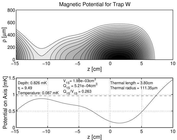
Figure 1: Potential and characteristics of the $1S$ sample in Trap W. The trap threshold is set by a 20 MHz rf field. Although calculations indicate that the magnetic trap threshold is below the rf threshold, the probability of an atom escaping over the magnetic saddlepoint is small compared to the probability of rf ejection, and the rf frequency effectively determines the threshold energy.

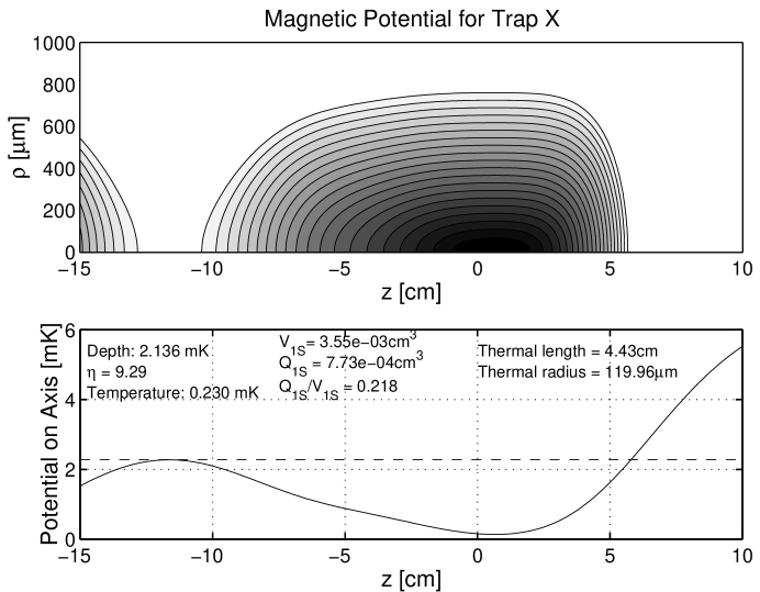
Figure 2: Potential and characteristics of the $1S$ sample in Trap X.

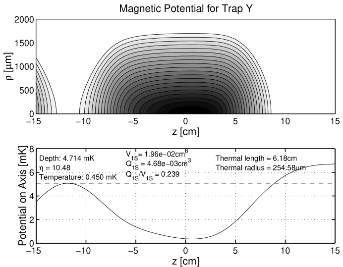
Figure 3: Potential and characteristics of the $1S$ sample in Trap Y.

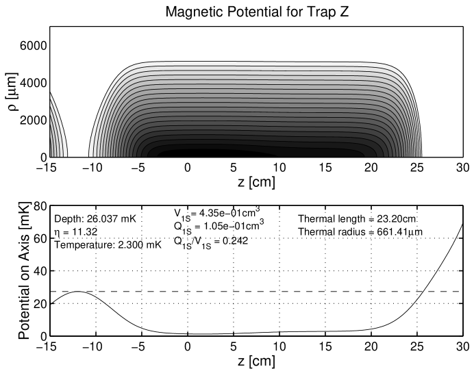
Figure 4: Potential and characteristics of the $1S$ sample in Trap Z.

The four magnetic traps chosen for detailed studies are known as Traps W, X, Y, and Z. In each trap, a ground state sample was prepared according to a consistent procedure, and metastable clouds were excited in this sample. The label “Trap W” will sometimes be used below to mean “the sample in Trap W.” The trap shapes and some parameters of the $1S$ cloud are shown in Figs. 1, 2, 3, and 4.

In order to determine collisional rate constants from the metastable decay, it is important to know the $1S$ density and temperature for each sample. Both parameters are needed to calculate the spatial distribution of the metastable cloud; these calculations will be detailed in Ch. 4. To determine the metastable density, it is also necessary to know the detection efficiency for metastables. The calibration of the detection efficiency presented in Sec. 4 requires knowledge of $N_{1S}$, the initial number of atoms in the sample. To find $N_{1S}$, the peak density $n_{1S}$ can be multiplied by the numerically calculated effective volume $V_{1S}$. The measured temperature and $1S$ density, together with $V_{1S}$ and $N_{1S}$, are summarized for the four traps in Table 1.

Trap	$T$ (mK)	$n_{o,1S}\ (\times 10^{13}$ cm-3)	$V_{1S}\ ($cm${}^{3})$	$N_{1S}\ (\times 10^{12})$
W	0.087	6.5	0.0020	0.13
X	0.23	4.1	0.0036	0.15
Y	0.45	2.5	0.020	0.49
Z	2.3	1.3	0.44	10

Table 1: Temperature, initial peak $1S$ density, effective $1S$ volume, and initial $1S$ atom number for the samples in which metastable decay behavior was studied in detail. The accuracy of the values in this table is discussed in the text.

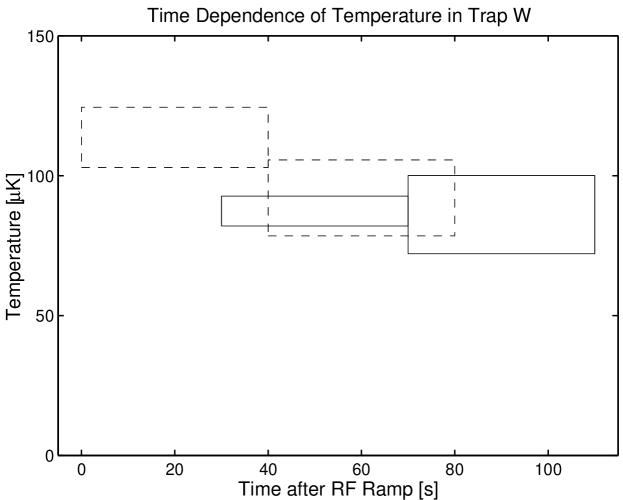
Figure 5: Temperature determined from Doppler-sensitive scans in Trap W for a sample probed immediately after the rf reached its final value (dashed) and for a sample probed after the rf was already at its final value for 30 s (solid). The horizontal extents of the rectangles indicate the boundaries of the 40 s time bin used for each temperature determination, and the vertical extents indicate the error bars. Considerable cooling occurs in the first 30 s after the rf ramp.

When measuring the temperature or density of a sample, it is important to ensure that the temperature has reached an equilibrium value which is maintained during the measurement. After the end of an evaporation sequence in which the trap depth is ramped downward, the sample will continue to cool for a time up to tens of seconds as the temperature asymptotically approaches an equilibrium value. This cooling has been observed directly in Trap W by scanning the excitation laser frequency repeatedly across the Doppler-sensitive line for about 1 minute after the evaporation ramp (Fig. 5). The average temperature during a given time interval was found by fitting the lineshape accumulated during the interval to a Gaussian, as in Fig. 5. In the case of Traps W, X, and Y, the standard practice was to hold the sample for 30 s after the evaporation ramp to allow equilibrium to be reached. At higher temperatures, evaporation proceeds more efficiently, and the sample is expected to be near equilibrium throughout the evaporation sequence. For this reason, no hold time was employed for Trap Z.

The temperatures of the equilibrated samples were determined by a combination of methods. For Trap W, which involved the coldest sample, the temperature was determined with an uncertainty of 5% from a Gaussian fit to the Doppler-sensitive $1S$-$2S$ line (Fig. 5). In the case of Trap X, the temperature was found by comparing the width of the Doppler-free $1S$-$2S$ lines for low density samples in it and Trap W (Fig. 4). The temperature extracted in this way agrees well with the trap depth divided by the equilibrium value of $\eta$, determined self-consistently from numerical simulations of a cylindrical quadrupole trap uniform in $z$ [29]. For higher temperature samples, the most reliable way to determine temperature at present is to obtain $\eta$ from simulations and use $kT=U_{t}/\eta$, where $U_{t}$ is the trap depth. This was done for Traps Y and Z. The estimated uncertainty in the temperatures for Traps X, Y, and Z is 10%.

Once the temperature of a sample is known, the $1S$ density can be determined by the bolometric method described in Sec. 3. The densities in Table 1 were determined this way. They have an estimated total uncertainty of 20%. Some of this uncertainty stems from systematic uncertainty in the dipolar decay constant and affects all of the density measurements in the same way; the measured densities should be accurate to 10% relative to each other.

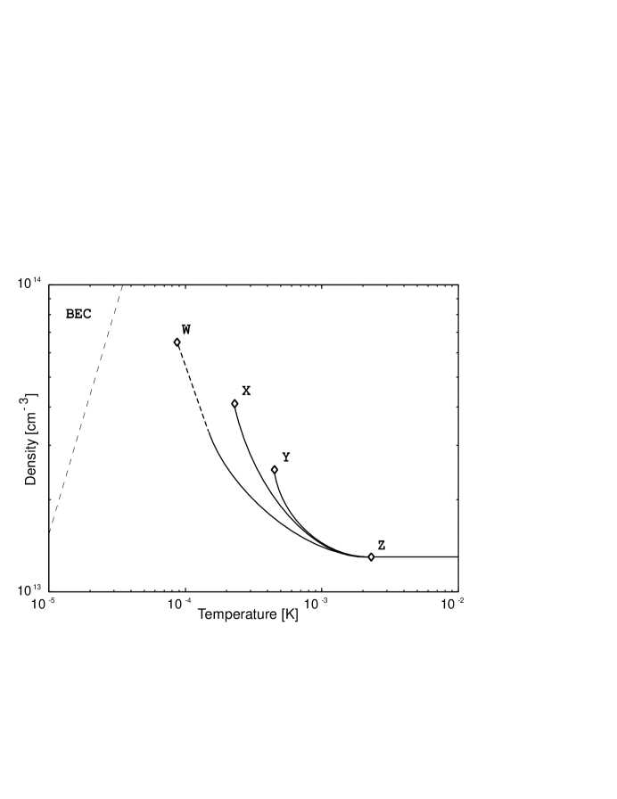
Figure 6: Location of ground state samples in phase space. The solid lines roughly indicate the trajectory of the samples during magnetic saddlepoint evaporation, originating from higher temperatures at right. A dashed line denotes the approximate rf evaporation trajectory of Trap W. A longer dashed line marks the boundary between the BEC and normal phases of the gas.

Values for the effective volume of the $1S$ cloud were obtained by numerical evaluation of $V_{1S}=\int$exp$(-U({\bf r})/kT)$ over the trap region. Since the gravity gradient (12 $\mu$K/cm) is not strong enough to significantly distort the trapping potentials at these temperatures, it was neglected in the calculations. The uncertainty in $V_{1S}$ is dominated by the temperature uncertainty. For small changes in $T$, numerical calculations show that $V_{1S}\sim T^{2}$ in all of the traps. Thus, $V_{1S}$ is accurate to about 10% for Trap W and 20% for the other traps. The number of atoms $N_{1S}$ in each trap was obtained by multiplying $n_{o,1S}$ by $V_{1S}$. Since the fractional uncertainties in $n_{o,1S}$ and $V_{1S}$ are essentially independent, we can add them in quadrature to find that the accuracy of the $N_{1S}$ values is 20-30%, closer to 20% for Trap W, and closer to 30% for the others.

A phase space representation of the four standard samples is shown in Fig 6. To prepare the sample in Trap W, an rf evaporation field was ramped from 35 MHz to 20 MHz and then held constant at 20 MHz for the duration of measurements. No rf evaporation was employed in the other traps. Although Trap W is considerably colder than Trap X, it contains almost as many atoms. This is because Trap W has less radial compression than Trap X. For Traps W, X, and Y, the energy of the trap minimum was determined by slowly sweeping the rf frequency upward from near DC until atoms were ejected from the sample and observed on the bolometer. In each of these traps, the minimum was found to be consistently 180-200 $\mu$K lower than the value predicted by numerical calculations based on the magnet currents. This discrepancy is assumed to be due either to uncertainty in the magnet geometry or to a stray field component pointing along the trap axis. For Trap Z, the trap minimum was estimated by subtracting 200 $\mu$K from the numerically calculated trap minimum.

2 Density-Dependent Decay Rates

To measure a two-body loss process in metastable H, it is important to have close control of not only the one-body decay rate and but also the $2S$ density. A first goal for our experiments was to see a systematic effect on metastable decay due to density. In this section, it is shown how the effective decay rate varied in each trap over the achievable $2S$ density range. More specifically, an effective decay rate is calculated as a function of the metastable signal in a decay curve. To a first approximation, the signal is simply proportional to the $2S$ density in the trap.

The density of metastables excited by a UV laser pulse varies during the excitation phase for several reasons. First, the ground state sample density decreases over many seconds due to dipolar decay. Second, the laser frequency is generally scanned back and forth across the center of the Doppler-free $1S$-$2S$ resonance. This allows the line center frequency relative to the laser’s reference cavity to be established in each trap cycle. The relative frequency drifts typically $\sim 20$ kHz per hour, measured at 243 nm. Since the laser frequency is stepped after each decay curve measurement, the detuning is stepped, and the excitation rate changes. Finally, there are sources of noise operating on a time scale which is short compared to the time required to make a decay measurement. These include fluctuations in the laser power and the overlap of the counterpropagating UV beams.

In order to obtain enough signal-to-noise for a useful analysis, the decay curves from the data set for a given trap must be grouped or “binned” together. To look for an effect dependent on the number of metastables excited, the decay curves can be binned according to the total number of metastable signal counts in each decay curve. This means that decay curves corresponding to approximately the same initial density are averaged together. Next, the average decay curve for each signal bin is fit with a model function. For a preliminary analysis, we use a simple exponential decay function

$$s(t)=A_{o}e^{-\alpha t}$$ (1)

as a model, where $s(t)$ is the number of signal counts at a time $t$ following the laser pulse, and the free parameters are an effective decay rate $\alpha$ and initial signal amplitude $A_{o}$. Even when the decay curve is distinctly nonexponential, the quantity $1/\alpha$ derived from a fit provides a useful measure of the lifetime of the metastable cloud. For cases where the decay is well described by Eq. 1, $\alpha$ can be interpreted as the total rate of one-body metastable loss processes.

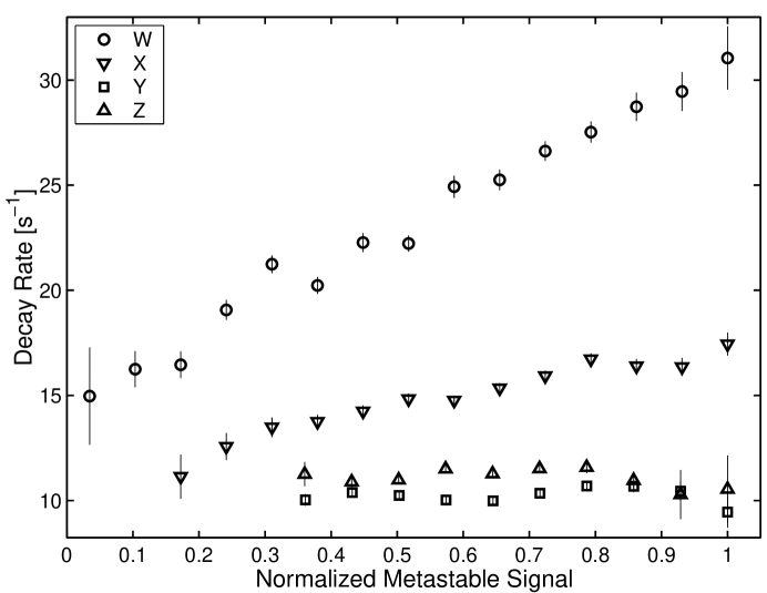
Figure 7: Effective decay rate $\alpha$ determined by fitting Eq. 1 to decay curves recorded in Traps W, X, Y, and Z. The curves were binned according to the total metastable signal in each decay curve. Error bars reflect only the statistical uncertainty in the data. The lower horizontal edge of the plot corresponds to the natural $2S$ decay rate of 8.2 s^-1. For this figure, the metastable signal has been normalized to the peak signal observed in each trap. The peak metastable density corresponding to the peak signal of Trap W is about $2\times 10^{9}$ cm^-3. The peak densities for Traps X, Y, and Z are roughly 10, 40, and 80 times larger, respectively.

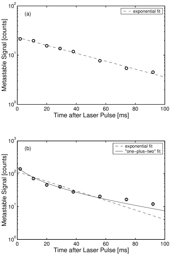
Figure 8: Average decay curves at two different signal levels in Trap W. The parent data set was gathered over five trap cycles, and the error bars account for only statistical error. For the curve in (a), more than 60 individual decay measurements have been averaged, and the statistical errors are smaller than the markers; non-statistical scatter is evident. For (b), the curve is the average of the two decay measurements in the data set with the largest signal. In case (b), where the initial metastable number is more than 6 times larger, a “one-plus-two” model fits the data better than a simple exponential. The one-plus-two model (see Sec. 1) incorporates terms corresponding to both one- and two-body loss, and it assumes the shape of the $2S$ cloud is static. In reality, the $2S$ distribution flattens somewhat as the cloud decays, and it is not surprising that the model deviates from the data at long wait times (Sec. 3).

Figure 7 summarizes the results for decay rates determined from fits to a simple exponential. The most dense metastable cloud is excited in Trap W, which contains the coldest, most dense ground state sample. In this trap, there is a clear monotonic increase of the effective decay rate with the number of metastables excited. For Trap X, which is warmer and less dense, the maximum decay rates are not as large, but the same trend with metastable signal is present. In the warmest and least dense samples, there is only a small increase in decay rate at the largest metastable population achievable in those traps.

It should be mentioned that the observed dependence of decay rate on metastable number is not a consequence of correlated variations in ground state sample density. To generate Fig. 7, all metastable decay curves with approximately the same initial metastable signal were binned together without regard to the ground state density, which decayed over the course of each laser scan from the initial values in Table 1. For each ground state density, a range of metastable populations was generated by varying the laser detuning.

Since $2S$ density increases with $2S$ signal in a given trap, the data indicate the presence of metastable loss processes which depend on the metastable density. The effect is strongest in Trap W, where the largest metastable densities were achieved. As will be explained in Sec. 3, a numerical simulation can be used to calculate the spatial distribution of $2S$ atoms for a given trap and laser geometry. This distribution can be integrated to obtain the effective volume of the metastable cloud. For resonant excitation, the peak number of metastables excited in a laser pulse is 50-70% larger in Trap W than in Trap Z, while the volume occupied by the $2S$ cloud in Trap W is $\sim 60$ times smaller (assuming perfect overlap of the counterpropagating UV beams). This means that the peak metastable density achieved in Trap W may be as much as 100 times larger than in Trap Z.

Qualitatively, the increase in peak decay rate going from Z to W is consistent with the existence of two-body inelastic processes which become increasingly significant at higher $2S$ densities. The data could also be consistent with an inelastic rate constant which increases with decreasing temperature. However, theoretical predictions for the relevant inelastic processes indicate that the rate coefficients should be nearly independent of temperature in the temperature range of these experiments (Fig 1).

In Traps W and X, the decay curves were observed to be exponential for low $2S$ signal and distinctly nonexponential at high $2S$ signal. This is illustrated in the semi-logarithmic plots of Fig. 8. In Fig. 8(a), the data is well fit by a simple exponential. For the decay curve starting at high signal in Fig. 8(b), there is a clear departure from an exponential. The data is better fit with a model which has a fixed one-body decay parameter and a free two-body parameter (“one-plus-two model”). The procedure for fitting to this model and extracting a $2S$-$2S$ inelastic rate constant is described in the following chapter.

Chapter 4 Analysis of Metastable Loss Dynamics

In order to determine the loss rate constant $K_{2}$ associated with $2S$-$2S$ inelastic collisions, it is convenient to first assume that the metastable cloud shape does not change as it decays. This allows the decay data to be fit by a simple model incorporating both one-body and two-body loss terms. The one-body parameter of the model can be fixed at the exponential decay rate inferred from the data for the limit of zero metastable density. With the one-body parameter fixed, the two-body parameter is easily determined from fits to decay curves. To find $K_{2}$, it is also necessary to know the geometry of the metastable cloud and the detection efficiency for metastables; these pieces of information establish the link between the $2S$ density and the observed signal. As will be explained in this chapter, the geometry and detection efficiency are difficult to determine precisely, and this gives rise to much of the uncertainty in the final values for $K_{2}$. Some more uncertainty arises because the $2S$ spatial distribution flattens significantly during a decay, and it is necessary to apply a correction factor based on a dynamic simulation of the cloud. Nevertheless, it is possible to determine $K_{2}$ to within a factor of about 2 with our data, and the results are compatible with the current state of theory. It is also possible with our data to set limits on the loss rates due to $1S$-$2S$ inelastic collisions. The details of the analysis follow.

1 One-Plus-Two Model

The extraction of a rate constant from the decay data is straightforward if we assume that (1) loss occurs solely due to a combination of one- and two-body processes (“one-plus-two model”) and (2) the shape of the metastable cloud is constant in time (“static approximation”). Three-body loss is not expected to play a role at the metastable densities achieved to date ($\sim 10^{11}$ cm^-3 or less). If the $2S$ distribution in the trap and the detection efficiency are known, then a total two-body loss constant in terms of density can be computed from the two-body parameter in the model.

In the static approximation of the one-plus-two model, the decay of the metastable signal is described by

$$\dot{s}=-\alpha_{1}s-\alpha_{2}s^{2},$$ (1)

where $\alpha_{1}$ and $\alpha_{2}$ are, respectively, the one- and two-body fit parameters. The solution to Eq. 1 is

$$s(t)=\frac{\alpha_{1}A_{o}e^{-\alpha_{1}t}}{\alpha_{1}+\alpha_{2}A_{o}(1-e^{-\alpha_{1}t})}.$$ (2)

Since $\alpha_{1}$ and $\alpha_{2}$ are highly correlated, it is not useful to vary both of these fit parameters simulataneously. Fortunately, $\alpha_{1}$ can be determined by extrapolation of effective decay rates $\alpha$ to the limit of very low metastable density; this will be explained more fully in Sec. 5. The parameter $\alpha_{1}$ represents the background one-body decay rate which occurs in a given trap regardless of the metastable density. With the fixed value for $\alpha_{1}$, the decay curves for all initial $2S$ densities can subsequently be fit with Eq. 2, using $\alpha_{2}$ and $A_{o}$ as free parameters. This was the procedure used to determine the solid curve in Fig. 8(b).

2 Two-Body Loss Constant in the Static Approximation

As discussed in Sec. 4, the relative spatial distribution of the metastable cloud evolves during its lifetime due to diffusion and two-body loss. For the purposes of extracting a value for the two-body loss constant from the decay data, however, we start with the simplifying assumption that the relative $2S$ distribution is static in time. The effect of metastable cloud dynamics will be considered afterwards in Sec. 3.

The desired two-body loss constant, $K_{2}$, is defined so that it gives the total local rate of $2S$ density change due to two-body processes:

$$\Bigl{.}\dot{n}_{2S}({\bf r})\Bigr{|}_{\rm two-body}=-K_{2}n_{2S}^{2}({\bf r}).$$ (3)

In terms of the normalized metastable distribution $f_{2S}({\bf r})=n_{2S}({\bf r})/n_{o,2S}$, where $n_{o,2S}$ is the peak density, the two-body loss from the entire trap is

$$\Bigl{.}\dot{N}_{2S}\Bigr{|}_{\rm two-body}=-K_{2}n_{o,2S}^{2}\int f_{2S}^{2}({\bf r})\,d^{3}{\bf r},$$ (4)

where $N_{2S}$ is the metastable population. Since the peak density cannot be measured directly in the current experiments, it is useful to rewrite the right-hand-side of Eq. 4 in terms of $N_{2S}$. Making use of the effective volume definitions

$$V_{2S}=\int f_{2S}({\bf r})\,d^{3}{\bf r}=\frac{N_{2S}}{n_{o,2S}}$$ (5)

and

$$Q_{2S}=\int f_{2S}^{2}({\bf r})\,d^{3}{\bf r},$$ (6)

we have

$$\Bigl{.}\dot{N}_{2S}\Bigr{|}_{\rm two-body}=-\frac{K_{2}Q_{2S}}{V_{2S}^{2}}N_{2S}^{2}=-\frac{K_{2}}{\zeta}N_{2S}^{2},$$ (7)

where $\zeta=V_{2S}^{2}/Q_{2S}$ is a quantity having units of volume and encapsulating all necessary information about the $2S$ cloud geometry. The quantity $\zeta$ is a measure of the spatial extent of the metastable distribution; $\zeta$ decreases as $f_{2S}(r)$ becomes more sharply peaked in space.

The quantity measured experimentally is $s(t)$, the number of metastable signal counts observed when quenching at time $t$ after excitation. The signal is proportional to the number of $2S$ atoms in the trap by the detection efficiency $\epsilon$:

$$s=\epsilon N_{2S}.$$ (8)

Since the signal decay due to two-body loss is given by

$$\Bigl{.}\dot{s}\Bigr{|}_{\rm two-body}=-\alpha_{2}s^{2},$$ (9)

it immediately follows that

$$K_{2}=\zeta\epsilon\alpha_{2}.$$ (10)

The method for determining $\alpha_{2}$ from the data has already been described. We turn our attention next to the calculations and measurements required to obtain $\zeta$ and $\epsilon$.

3 Spatial Distribution of Metastables

1 Monte Carlo Calculation of $2S$ Distribution

A lineshape simulation was developed by L. Willmann of the MIT Ultracold Hydrogen Group to calculate the $1S$-$2S$ excitation spectrum for realistic experimental conditions. The simulation can be used to calculate the spectrum due to atoms excited at different $z$ positions. If contributions for enough different $z$ positions are calculated, the distribution of metastables immediately following excitation can be extracted from the lineshape results.

The input parameters to the simulation include the laser field geometry, the trap shape, the sample temperature, and the chemical potential, which is related to the sample density by the Bose-Einstein distribution. The simulation is based on the principle that the contribution to the excitation spectrum by a single atom is proportional to the Fourier transform of the electric field experienced by the atom during the excitation pulse. Moreover, the cold-collision shift is incorporated by allowing the resonance frequency to vary during the pulse according to the trajectory of the atom in the trap; if ${\bf r}$(t) is the atom trajectory, the resonance frequency as a function of time is $\nu_{o}-\chi n_{1S}({\bf r}(t))$, where $\nu_{o}$ is the unperturbed resonance frequency and $\chi$ is the cold-collision shift per unit density. When the laser field intensity and instantaneous resonance frequency are sampled at a sufficient number of points along the trajectory, a Fast Fourier Transform (FFT) algorithm accurately produces the single-atom lineshape contribution.

In each simulation, a Monte Carlo routine first generates a density of trajectory states table with trajectories classified according to $z$, the maximum distance from trap center $\rho_{\rm max}$ during a complete “orbit”, and the orbital angular momentum $L$. The orbits are considered to occur at constant $z$, since the distance traveled by the atoms along $z$ during a laser pulse is small compared to the trap length scale. Momentum-changing collisions are neglected since typical collision times are longer than the laser pulse. Next, the FFT’s of a prescribed number of trajectories are computed in a second Monte Carlo procedure. The contribution of each FFT to the final spectrum is weighted according to the density of trajectory states and the Bose-Einstein distribution.

The lineshape simulation has produced spectra in good agreement with experimental spectra for a wide range of trap shapes, laser geometries, sample densities, and temperatures. For the purposes of the analysis presented here, sufficient accuracy in the $2S$ distribution is obtained for a given set of input parameters after about one hour of CPU time on a computer which performs the FFT of a 1024-point trajectory every $\sim 50$ ms.

2 Results of Spatial Distribution Calculations

The Monte Carlo simulation provides the axial distribution of metastables in the trap. Under the assumption that a thermal distribution is established quickly in the radial direction, the distribution function $f_{2S}({\bf r})$ is easily calculated for the entire trap. Using the photoionization correction factor $C(z,t)$ described in Sec. 3, the distribution function is corrected for photoionization losses during the excitation pulse. Numerical integration can then be used to determine the geometry factor $\zeta$.

By varying the input parameters to the simulation, the sensitivity of $\zeta$ to various experimental uncertainties can be determined. The most important uncertainty by far is found in how well the focuses of the counterprograting UV beams are overlapped along $z$. The alignment of the beams to the trap axis can be done accurately using the imaging technique of Fig. 9, and the concave cell retromirror effectively fixes the centroid of the incoming and return focuses. However, it is difficult to ensure that no separation exists between the focuses. The present method of minimizing the separation is to match the sizes of the overlapped incoming and return beam modes in Telescope 2 of Fig. 8. This is accomplished by adjusting the length of the telescope. The estimated typical discrepancy in mode sizes for the decay measurements presented here is 10% or less, which translates into a separation of 1.8 cm or less between the two beam waists.

The dependence of the $2S$ spatial distribution on the separation of the laser focuses is illustrated for Trap W in Fig. 1. A separation of 1.8 cm produces a significant change since the local Doppler-free excitation rate depends on the product of incoming and return beam intensities, and the Rayleigh range is only 0.6 cm for the 21 $\mu$m waist radius. Values of $\zeta$ determined in this and other traps for zero laser detuning are summarized in Table 1.

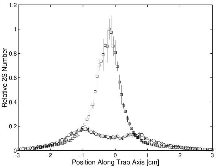
Figure 1: Relative number of metastables as a function of position relative to the trap minimum in Trap W. At each position, the Monte Carlo lineshape simulation was used to calculate the number of atoms excited assuming the laser focuses were perfectly overlapped (squares) and separated by 1.8 cm (circles) along $z$. The detuning of the laser from the $1S$-$2S$ resonance is zero, and the centroid of the focuses is located at -0.2 cm. Error bars indicate the scatter in the simulation results.

	$\zeta\,(10^{-3}$ cm${}^{3})$,	$\zeta\,(10^{-3}$ cm${}^{3})$,
Trap	$d_{\rm sep}=0$ cm	$d_{\rm sep}=1.8$ cm
W	2.0	4.3
X	3.3	6.4
Y	16	27
Z	150	250

Table 1: Results for the geometry factor $\zeta$ at zero laser detuning, calculated by numerical integration of $f_{2S}({\bf r})$. The spatial distribution function along $z$ was generated using the Monte Carlo lineshape simulation, and the radial distribution was assumed to be Maxwell-Boltzmann. The assumed separation of incoming and return laser focuses is denoted by $d_{\rm sep}$.

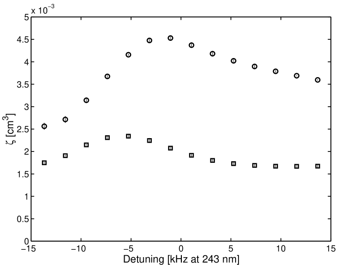
Figure 2: Values of $\zeta$ in Trap W as a function of laser detuning. Circles are for the case where the two laser focuses are separated along the trap axis by 1.8 cm, and squares indicate the case of perfect overlap. The two cases provide approximate upper and lower bounds for the true value of $\zeta$ in the experiment.

Though the laser field geometry is the most important factor in determining the shape of the metastable cloud, the shape also depends on laser detuning. This is a consequence of the cold-collision shift. The atomic resonance frequency of an atom passing in and out of a dense region of the ground state cloud is chirped by the changing cold-collision shift, which is proportional to the local density. In this way, the excitation spectrum of a single atom is both broadened and shifted. At red detunings (laser frequencies less than the unperturbed $1S$-$2S$ resonance frequency), the $2S$ distribution is slightly more concentrated near the trap minimum in $z$ than for zero detuning. This is because the high density near the trap minimum shifts the atomic resonances to lower frequency. At blue detunings the relative metastable distribution will generally again become more concentrated about the trap minimum since most of the excited atoms are ones whose resonances have been sufficiently chirped in a high density region.

Figure 2 shows the variation of $\zeta$ in Trap W over the range of detunings used for most $2S$ decay measurements. The dependence on detuning is stronger when the laser focuses are separated. In traps where peak densities are smaller and the ground state cloud extents are larger relative to the laser depth of focus, the dependence on detuning is less. For example, in Trap Z, $\zeta$ varies by less than 20% over the detuning range used in Fig. 2, even for focuses separated by 1.8 cm.

4 Measurement of Detection Efficiency

To obtain $K_{2}$ from $\alpha_{2}$ in the static approximation, it is crucial to know not only $\zeta$ but also the detection efficiency $\epsilon$. The detection efficiency completes the connection between the metastable signal, which we observe, and the metastable density.

While it is difficult to measure $\epsilon$ precisely with the current apparatus, it can be calibrated to better than a factor of 2 by depleting the ground state sample as quickly as possible through $1S$-$2S$ excitation. For an ideal measurement by this approach, the only significant loss mechanism would be excitation, and the detection efficiency would be given simply by the total number of signal counts observed divided by the initial number of atoms in the trap, $N_{1S}(0)$. However, even in cases where the depletion rate due to excitation is high, there can also be significant loss due to dipolar decay and due to laser heating of the trapping cell, which causes helium atoms to be evaporated from the cell walls. Another complicating factor in a real experiment is that a considerable fraction of the metastables relax back to the trapped $d$ ground state and are subsequently excited again (see Sec. 2). Finally, since the metastables are quenched after some wait time following the laser pulse, some correction needs to be made for the signal “missing” due to inelastic collisions of metastables during the wait time. The following paragraphs outline a method for extracting the detection efficiency which takes all these factors into account.

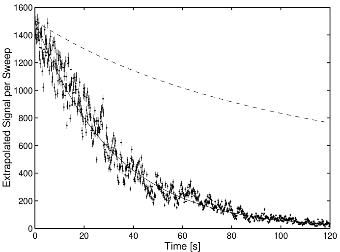
Figure 3: Decay of $1S$ cloud in Trap X undergoing resonant excitation. Each data point is the total number of signal counts in a sweep across resonance. The signal has been corrected for counts which were missed because of the delay time between excitation and quench pulses. Shown for comparison is the theoretical signal which would be observed in the absence of any laser-induced loss (dashed curve). Error bars indicate only the uncertainty due to counting statistics; significant non-statistical fluctuation in the signal is evident, believed due to optical alignment jitter which affects the overlap of incoming and return UV focuses. The average detection efficiency for this trap is obtained by integrating the fitted (solid) curve and dividing by the total number of atoms excited to the $2S$ state.

Figure 3 shows the results of a ground state depletion experiment in Trap X. The 243 nm laser frequency is swept back and forth across the central 10 kHz of the $1S$-$2S$ line, completing a sweep in one direction every 150 ms. Since the laser frequency remains near the center of the line, the sample is depleted quickly; after 120 s, only a few percent of $N_{1S}(0)$ remain in the trap. To analyze the data, the number of signal counts observed after each laser pulse was first corrected for the loss which occurs during the 5.4 ms wait time between excitation and quench pulses. This was done by extrapolating backwards in time using Eq. 2 with experimentally determined values of $\alpha_{1}$ and $\alpha_{2}$. Next, the extrapolated signal was summed across each laser sweep, and the results were fit with a smooth curve $y(t)$, shown in Fig. 3, where $t=0$ is the beginning of the depletion experiment. The quantity $y(t)$ serves as a distribution function of the $1S$-$2S$ signal in time.

To understand how the detection efficiency is extracted from $y(t)$, we consider its relationship to $W_{1S-2S}(t)$, the excitation rate at time $t$ averaged over a laser sweep:

$$\epsilon(t)=\frac{y(t)}{W_{1S-2S}(t)}.$$ (11)

We neglect here the small number of metastables lost during the excitation pulse itself. The detection efficiency is an increasing function of time, because the number of fluorescence photons “lost” due to radiation trapping decreases as the $1S$ density decreases (Sec. 2). It is useful to calculate the average detection efficiency $\bar{\epsilon}$ per metastable during the depletion experiment,

$$\bar{\epsilon}=\frac{\int W_{1S-2S}(t)\epsilon(t)\,dt}{\int W_{1S-2S}(t)\,dt}=\frac{\int y(t)\,dt}{\int\left[y(t)/\epsilon(t)\right]dt}\,.$$ (12)

The integration is to be taken over the duration of the experiment. Equation 12 can be written in terms of the initial detection efficiency $\epsilon(0)$ using

$$\epsilon(t)=\frac{1-F(t)}{1-F(0)}\,\epsilon(0),$$ (13)

where $F(t)$ is the fraction of fluorescence photons in the detection solid angle which are absorbed by the $1S$ cloud. The radiation trapping simulation described in Sec. 2 predicts $F(0)=0.22$ in Trap X with an uncertainty of 20% stemming primarily from uncertainty in the initial ground state density. This number is relatively insensitive to the sample temperature, the laser detuning, and the separation of the laser focuses. Results from simulations at several sample densities in Trap X were used to show $F(t)\simeq[N_{1S}(t)/N_{1S}(0)]F(0)$. The fraction of atoms remaining, $N_{1S}(t)/N_{1S}(0)$, can be obtained by taking $y(t)/y(0)$ and making a correction for the changing width of the $1S$-$2S$ line due to decreasing cold-collision shift. Substituting into Eq. 12, we obtain

$$\bar{\epsilon}=\left(\frac{\epsilon(0)}{1-F(0)}\right)\frac{\int y(t)\,dt}{\int[y(t)/(1-F(t))]\,dt}\,.$$ (14)

Now, Eq. 12 can be interpreted as equating the average detection efficiency with the total number of signal counts divided by the total number of atoms excited to the $2S$ state. We can write the total number of atoms excited as

$$\int W_{1S-2S}(t)\,dt=N_{1S}(0)-N_{d}-N_{l}+N_{r},$$ (15)

where $N_{d}$ is the total number of atoms lost to dipolar decay, $N_{l}$ is the number lost due to laser heating in the trapping cell, and $N_{r}$ is the number of relaxations back to the trapped $1S$ state when metastables are quenched. The small number of atoms remaining in the trap at the end of the depletion measurement are neglected. Substituting Eq. 15 into Eq. 12 yields an alternative expression for the average detection efficiency:

$$\bar{\epsilon}=\frac{\int y(t)\,dt}{N_{1S}(0)-N_{d}-N_{l}+N_{r}}\,.$$ (16)

The rate of relaxations back to the trapped sample is approximately given by $d_{r}W_{1S-2S}(t)$, where $d_{r}$ is the spatially-averaged branching ratio to $\left|1S_{d}\right\rangle$ for metastables in the quenching electric field. Thus,

$$N_{r}\simeq d_{r}\int{\frac{y(t)}{\epsilon(t)}\,dt}=\frac{d_{r}[1-F(0)]}{\epsilon(0)}\,\int{\frac{y(t)}{1-F(t)}\,dt}\,.$$ (17)

For Trap X, Monte Carlo simulations predict that $d_{r}\simeq 0.43$, virtually independent of sample density, temperature, laser detuning, and separation of the focuses. Equation 17 is not exact because the branching ratio is unknown for those metastables decaying before the quench field is applied. The resulting uncertainty is small, however, relative to other uncertainties in the detection efficiency determination.

The number of atoms lost to dipolar decay and the number lost to laser heating are calculated numerically from $N_{1S}(t)$, using

$$N_{d}=\frac{gQ_{1S}}{V_{1S}^{2}}\int N_{1S}^{2}(t)\,dt,$$ (18)

where $g$ is the dipolar decay constant, and

$$N_{l}=\frac{1}{\tau}\int N_{1S}(t)\,dt,$$ (19)

where $\tau$ is the time constant for sample decay due to laser heating. At the high laser power ($\sim 20$ mW) used to obtain the data in Fig. 3, $\tau$ was determined to be about 200 s by tuning the laser far off resonance and observing the depletion of the sample. Taking $N_{1S}(0)$ from Table 1, Eqs. 18 and 19 evaluate to $N_{d}=2.6\times 10^{10}$ and $N_{l}=2.3\times 10^{10}$ for this data.

By combining Eqs. 14, 16, and 17, the initial detection efficiency in Trap X is determined to be

$$\epsilon(0)=1.9^{+1.1}_{-0.6}\times 10^{-6}.$$ (20)

The errors are due predominantly to uncertainties in temperature and initial density. By comparing radiation trapping calculations for Traps W, X, Y, and Z, the detection efficiency can be predicted for the other traps as well (see Table 2). It turns out that $1-F(0)$ (and thus $\epsilon(0))$ is roughly constant across the traps. As the sample becomes cooler and denser along the evaporation pathway, it also becomes shorter along the trap axis, and the optical density seen by Lyman-$\alpha$ photons traversing the axis towards the detector remains nearly the same. We note that the detection efficiency for metastables at zero $1S$ density is simply $\epsilon(0)[1-F(0)]^{-1}=2.4\times 10^{-6}$, with relative uncertainties similar to those in Eq. 20.

Trap	$F$	$\epsilon(0)(\times 10^{-6})$
W	0.28	1.8
X	0.22	1.9
Y	0.26	1.8
Z	0.32	1.7

Table 2: Summary of initial detection efficiencies for the various samples. For Trap X, $\epsilon(0)$ was determined by the method described in the text. For the other traps, $\epsilon(0)$ has been scaled according to $(1-F)$, where $F$ is the fraction of fluorescence photons in the detection solid angle which are absorbed by the $1S$ cloud. While the absolute accuracy of the $\epsilon(0)$ values derives from the uncertainty of the Trap X measurement (lower relative error $\simeq 30$%, upper relative error $\simeq 60$%), the ratios of the values for different traps are estimated to have an uncertainty of only about 10%.

With knowledge of the detection efficiency, the population of a metastable cloud can be inferred from the number of signal photons detected during the quench pulse. In Trap W, for example, as many as 150 counts were observed for a single laser shot, implying $N_{2S}\simeq 8\times 10^{7}$. Depending on the separation of the laser focuses, the effective volume of the $2S$ cloud in Trap W lies between $4\times 10^{-4}$ and $1.2\times 10^{-3}$ cm³. This means that peak metastable densities as high as $\sim 10^{11}$ cm^-3 have been achieved.

5 Two-Body Loss: Experimental Results

1 $K_{2}$ in the Static Approximation

With values for $\zeta$ and $\epsilon$ in hand, we can finally turn our attention again to $\alpha_{2}$ and the determination of $K_{2}$.

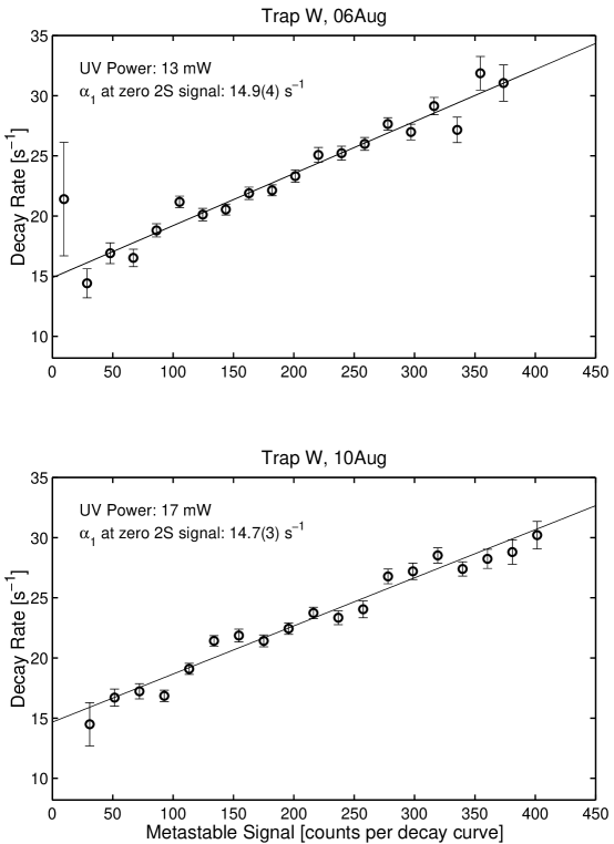
Figure 4: Determination of average $\alpha_{1}$ by extrapolation of exponential decay rates to zero metastable density for two complete data sets in Trap W. The data sets were taken four days apart under identical conditions, except that the excitation laser power was 30% larger in the lower plot. The values for $\alpha_{1}$ are in good agreement, indicating that systematics associated with laser power are insignificant. The fact that the peak signal increases by less than 10% for a 30% increase in UV power indicates that these experiments are in a saturation regime for metastable production.

Before fitting the decay curves of a given data set to extract $\alpha_{2}$, the fixed value for $\alpha_{1}$, the “background” one-body loss rate, must be chosen. This is accomplished by fitting decay curves at different metastable signal levels with simple exponentials and extrapolating the corresponding decay rates to zero metastable signal. Plots of the best-fitting exponential decay rate $\alpha$ against metastable signal show, to a good approximation, that decay rates are linear with metastable signal, suggesting that linear extrapolation is a reasonable way to obtain $\alpha_{1}$.

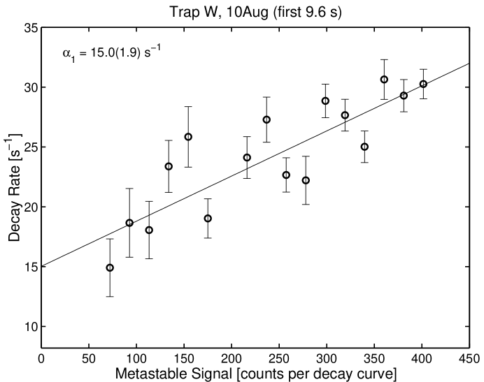
Figure 5: An extrapolation similar to those in Fig. 4, but using decay curves from only the first 2 sweeps across the $1S$-$2S$ resonance, during which time the ground state density is known and relatively constant. Error bars on the decay rates are derived assuming only statistical errors in the decay curves, which means they are smaller than the true uncertainties. To avoid underestimating the error on $\alpha_{1}$, the uncertainty derived from the linear fit has been multiplied by the square root of the $\chi^{2}$ statistic of the fit.

Figure 4 shows linear extrapolations of the one-body rates to zero signal for two different data sets in Trap W. The resulting values of $\alpha_{1}$, employing decay curves from the entire data sets, are in good agreement. Since the data sets were taken on different days with different laser powers, the agreement provides evidence that (1) trap conditions, including stray electric fields, were relatively constant over a period of several days and (2) systematic effects associated with changes in the laser power are small.

The decay data compiled to create Fig. 4 was taken continuously over the first 120 s after sample preparation at a rate of one decay curve every 0.8 s. The ground state sample depletes substantially during this time due to dipolar decay. In Trap W, for example, the peak ground state density decreases by two-thirds. To minimize the role of systematics associated with changes in the ground state sample density, only decay curves taken within the first 10-15 s after sample preparation were considered in the determination of $K_{2}$. In all of the traps, the $1S$ density decreased by less than 20% in the time required to acquire this data subset. Furthermore, since the laser duty cycle was only 2%, ground state losses due to laser heating and excitation were insignificant. Since $\alpha_{1}$ can vary as the ground state density changes (see Sec. 6), the same 10-15 s subset of decay curves was employed to determine a value of $\alpha_{1}$ to use when fitting to the one-plus-two model. As an example, Fig. 5 shows the linear extrapolation used to find $\alpha_{1}$ for the first 9.6 s of a Trap W data set.

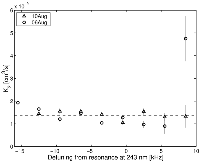
Figure 6: Experimental results for the two-body loss constant $K_{2}$ in Trap W, derived in the static approximation. The decay data has been binned by laser detuning. A value of $1.8\times 10^{-6}$ has been used for $\epsilon$, and $\zeta$ has been calculated for each laser detuning assuming perfect overlap of the laser focuses (see Fig. 2). Results from two data sets with different laser powers are in reasonable agreement. The error bars on individual points derive from the fits to the one-plus-two model which include only statistical uncertainties. The weighted average (dashed line) of all points is $1.4\times 10^{-9}$ cm³/s. The error bars on $K_{2}$ are discussed in the text.

After $\alpha_{1}$ has been determined, the decay data is fit to the one-plus-two model. To accumulate enough statistics, a typical data set encompasses five consecutive trap cycles. The decay curves taken during the first two or three sweeps across resonance in each trap cycle are binned according to laser detuning. The resulting curves are fit with Eq. 2, using only $\alpha_{2}$ and $A_{o}$ as free parameters. The values for $\alpha_{2}$ at different laser detunings are substituted into Eq. 10 to obtain values for $K_{2}$ in the static approximation. Since the $1S$ density and the cold-collision shift do not change much in 10-15 s, it is a good approximation to assume that the value of $\zeta$ calculated for each detuning is constant. As shown in Fig. 6, the $K_{2}$ values are relatively independent of detuning, indicating that the variations in metastable cloud shape with detuning are reasonably accounted for by the spatial distribution calculations. The experimental value of $K_{2}$ for a given trap is taken to be the weighted average of the values determined at different detunings.

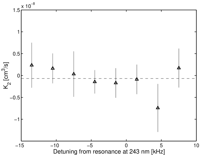
Figure 7: Determination of $K_{2}$ in Trap Z assuming perfect overlap of the laser focuses and a detection efficiency $\epsilon=1.7\times 10^{-6}$. The weighted average (dashed line) is consistent with zero within the statistical uncertainties. By summing the systematic uncertainties, an upper limit for $K_{2}$ of $7\times 10^{-9}$ cm³/s is obtained.

Table 3 summarizes the results for $K_{2}$ obtained in the static approximation. The asymmetric error bars for Traps W and X derive mostly from systematic uncertainties, which are summarized in Sec. 2. In traps Y and Z, the weighted average of $K_{2}$ is consistent with zero (Fig. 7). Nevertheless, an upper limit for $K_{2}$ has been established by linear addition of the uncertainties in $\alpha_{2}$, $\epsilon$, and $\zeta$ appropriate for these traps. If $K_{2}$ maintains the same order of magnitude across the temperature range spanned by Traps W, X, Y, and Z, it is not surprising that two-body loss is difficult to detect in Traps Y and Z, given the much lower metastable densities and the sizeable systematics.

At red detunings larger than 10 kHz and blue detunings larger than 5 kHz, the metastable cloud in Trap W appeared sometimes to decay very rapidly in the first 10-20 ms after excitation, implying values of $K_{2}$ far above the wighted average. For example, note the outlying point in the most blue-detuned bin of Fig. 6. The origin of these anomalously steep decay curves is not yet understood. Perhaps at large detunings either (1) the metastable distributions calculated by Monte Carlo simulation are inaccurate or (2) transient redistribution of the $2S$ cloud in the first $\sim 10$ ms somehow leads to an accelerated decay of the observed fluorescence. The statistical weight of the anomalously fast decay curves is small, however, and their inclusion in the weighted average has little effect on the final results.

Trap	$T$ (mK)	$K_{2}$ $(10^{-9}$ cm3/s)
W	0.087	$1.4^{+1.3}_{-0.5}$
X	0.23	$0.74^{+0.70}_{-0.35}$
Y	0.45	$<2$
Z	2.3	$<7$

Table 3: Results for $K_{2}$ in the static approximation. The sources of uncertainty will be discussed in Sec. 2.

A check was made to see if the results for $K_{2}$ were biased by the fact that only the first few time points in the decay curve are sensitive to two-body decay. For example, consider that during the first 30 ms following excitation of a large metastable population in Trap W, the $2S$ number decays by a factor of 4. The two-body loss rate, which depends locally on the square of the metastable density, decreases dramatically during this time. For the remaining $\sim 60$ ms of the measured decay curve, one-body loss dominates. The check consisted in repeating the measurements in Trap W with eight wait times concentrated in the first 30 ms of the decay. The resulting value for $K_{2}$ agreed to within 10% of the previous measurements made with eight time points distributed across 92 ms. This confirms that the results were not significantly biased by the chosen distribution of wait times.

2 Uncertainties: Static Approximation

The uncertainties relevant to determination of $K_{2}$ under the assumption of a static $2S$ cloud shape are summarized for Trap W in Table 4. Most of the uncertainties are systematic in nature, stemming from imprecise knowledge of the excitation geometry and also of the sample temperature and density. The uncertainties which enter through $\zeta$ have been estimated by varying the inputs to the numerical calculation of the $2S$ distribution. The overall error bars are asymmetric due to asymmetric uncertainty in the detection efficiency and the fact that laser misalignments generally lead to an increase in $\zeta$.

Source of Uncertainty	Est. Contribution to	Est. Contribution to
	Lower Rel. Error (%)	Upper Rel. Error (%)
$\alpha_{2}$	12	12
$\epsilon$	32	58
$\zeta$
overlap of waists	0	75
size of waists	16	16
trap shape	5	5
cold-collision shift	4	4
trap/laser focus offset	0	3
$n_{1S}$	3	3
$T$	2	2
laser linewidth	$<1$	$<1$
photoionization	$<1$	$<1$
Total Relative Error (%)	38	97

Table 4: Uncertainties for the static approximation determination of $K_{2}$ in Trap W. To obtain the total relative error, the values in the table are added in quadrature, excluding the $\zeta$ contributions from ground state density $n_{1S}$ and the temperature $T$ (see explanation in text). The “overlap of waists” refers to the separation of incoming and return laser focuses along $z$, while the “trap/laser focus offset” refers to the location of the laser focuses in $z$ with respect to the trap minimum. The contribution labeled “cold-collision shift” is due to uncertainty in the parameter which relates the shift of the $1S$-$2S$ transition to the $1S$ density.

The uncertainty budget for Trap X is similar to Table 4. For Trap X, however, the uncertainty in $\alpha_{2}$ is 30%, and the upper relative error associated with overlap of the focuses is 65%. The smaller relative errors associated with $\zeta$ have not been explicitly calculated for Trap X, but are assumed not to differ significantly from those in Trap W. In both of these traps, the uncertainty in $\alpha_{2}$ stems mainly from the imprecise extrapolation of $\alpha_{1}$; the parameters $\alpha_{1}$ and $\alpha_{2}$ are highly correlated in the one-plus-two model.

With a couple exceptions, the uncertainties in Table 4 are assumed to be uncorrelated. The errors in ground state temperature and density are responsible for most of the uncertainty in $\epsilon$. However, the $T$ and $n_{1S}$ contributions to $\epsilon$ are somewhat anti-correlated with the corresponding contributions to $\zeta$. In other words, an error in $T$ (or $n_{1S}$) leads to errors in $\epsilon$ and $\zeta$ with opposite signs. To be conservative, the possibility of small partial cancellations is ignored by neglecting the $n_{1S}$ and $T$ contributions to $\zeta$. The estimated total relative error is found by adding all other uncertainties in quadrature.

3 Effects of the Changing Metastable Cloud Shape

As acknowledged before, the shape of the metastable cloud changes while it is decaying. Although thermal equilibrium is maintained in the radial direction, the shape of the cloud evolves in the axial direction due to diffusion and to two-body loss, which occurs preferentially where metastable density is highest. To estimate the corrections which must be made to the static approximation analysis in order to account for these dynamics, a numerical simulation of the decaying metastable cloud was developed.

The simulation begins with a distribution $f_{2S}({\bf r})$, calculated for a particular trap, excitation geometery, and laser detuning by the Monte Carlo method of Sec. 3. Other inputs to the simulation include the peak ground state density $n_{o,1S}$, a putative value for $K_{2}$, a uniform one-body loss rate $\alpha_{1}$, a one-dimensional diffusion parameter, the detection efficiency $\epsilon$, and $s_{o}$, the number of signal counts which would be experimentally observed when quenching immediately after the excitation pulse.

The diffusion parameter is the proportionality constant $C_{\rm diff}$ in the relation

$$\sigma_{z}(n_{a,1S},t)=C_{\rm diff}\left(\frac{t}{n_{a,1S}}\right)^{1/2},$$ (21)

where $\sigma_{z}$ is the rms diffusion length of $2S$ atoms along $z$ in a background $1S$ gas, $t$ is the corresponding diffusion time, and $n_{a,1S}$ is the $1S$ density on the trap axis. Using the Monte Carlo diffusion simulation described in Sec. 2, $C_{\rm diff}$ was calculated to be $4.3\times 10^{5}$ (cm ms)^-1/2 at the minimum of Trap W. This constant has some dependence on the local radial curvature of the trap. However, for the purpose of simulating the evolution of the metastable cloud in the presence of large two-body losses, it is a good approximation to neglect the variation of $C_{\rm diff}$ with $z$.

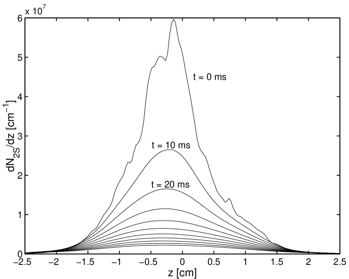
Figure 8: Results from a dynamic simulation of the time evolution of a metastable cloud in Trap W. The plot depicts the distribution of $2S$ atoms, $dN_{2S}/dz$, in the $z$ direction as the population decays; the distribution is shown at 10 ms intervals from $t=0$ ms to $t=100$ ms following the excitation pulse. The ripples on the initial curve are due to the finite number of trajectories used in the Monte Carlo calculation of the $2S$ spatial distribution. Diffusion and loss processes in the simulation quickly smooth out the ripples. In this example, the laser focuses were assumed to be perfectly overlapped, and the initial number of $2S$ atoms was $7\times 10^{7}$, which approximates the largest number of metastables excited in the decay measurements.

In the simulation, the initial number of metastables $s_{o}/\epsilon$ is used to establish an initial absolute $2S$ distribution. At any given time, if the number distribution $dN_{2S}(z)/dz$ is known, the density distribution $n_{2S}({\bf r})$ can be calculated everywhere assuming that the radial distribution is Maxwell-Boltzmann. For each step in time $\Delta t$, the total number of atoms lost to one- and two-body processes is numerically integrated as a function of $z$, and $dN_{2S}(z)/dz$ is adjusted accordingly. To account for diffusion during the time step, the distribution in $z$ is also convoluted with a Gaussian of rms width $\sigma_{z}(z,\Delta t)$, whose $z$ dependence comes from $n_{a,1S}(z)$. The time evolution of $dN_{2S}(z)/dz$ for an example simulation in Trap W is shown in Fig. 8.

To compare the cases of “static” and “dynamic” evolution of the metastable cloud, the dynamic simulation also evolves the number in a static cloud starting from the same initial conditions. At each time step, loss is calculated in the static cloud in the same way as in the dynamic cloud, but only the total $2S$ number is adjusted and not the relative distribution. The static and dynamic evolutions for the initial conditions of Fig. 8 are compared in Fig. 9. After each step in time, the geometry factor $\zeta$ is calculated for both static and dynamic cases. Since diffusion and two-body loss cause $f_{2S}({\bf r})$ to become less sharply peaked, $\zeta$ increases with time in the dynamic simulation. The rate of increase slows as the peak $2S$ density drops and two-body loss becomes less important relative to one-body loss. The effect of the increase in $\zeta$ in the dynamic case is to decrease the two-body loss rate relative to the static case (Eq. 7). This effect is only important, however, during the early part of the decay when two-body loss dominates.

Figure 9: Simulation results for $\zeta$ and $N_{2S}$ in dynamic (solid curves) and static (dashed curves) evolution of the metastable cloud. The initial conditions are the same as those of Fig. 8.

Figure 10: Fits of the one-plus-two model to simulated decay data derived from the $N_{2S}(t)$ curves of Fig. 9. In both cases, the one-body constant $\alpha_{1}$ has been fixed at an experimental value of 15 s^-1, and the one-plus-two model is an excellent fit to the simulation results. The ratio of $\alpha_{2}$ values determined in the two cases provides a correction factor for $\alpha_{2}$ in the static approximation.

As illustrated in Fig. 10, the results of the simulation can be used to calculate a dynamic correction for $\alpha_{2}$ in the one-plus-two model (Sec. 1). In the figure, the simulated $N_{2S}(t)$ curves have been multiplied by $\epsilon$ at the experimental wait times to obtain decay curves similar to those in the experiment. Applying statistical error bars and using an experimentally determined value for $\alpha_{1}$, the simulated static and dynamic decay curves are fit to the one-plus-two model to find $\alpha_{2}$ in each case. A dynamic correction factor $f_{\rm dc}$ can be defined as follows:

$$f_{\rm dc}=\frac{\alpha_{\rm 2,static}}{\alpha_{\rm 2,dynamic}}.$$ (22)

The values of $\alpha_{2}$ extracted from fits of the one-plus-two model to experimental decay curves can be multiplied by $f_{\rm dc}$ to account for the flattening of the metastable distribution as the cloud decays.

The simulation was executed many times with the parameters of Traps W and X to find $f_{\rm dc}$ as a function of laser detuning. These results were used to correct the static approximation values for $K_{2}$, and a new weighted average $K_{2}$ was determined for each trap. The input parameters to the simulation were varied to estimate the uncertainty in the overall correction to $K_{2}$. It was found that the static approximation values of $K_{2}$ must be multiplied by $1.35$ and $1.30$, respectively, to correct for dynamics in Traps W and X. The uncertainty in these factors is estimated to be 10%. For Traps Y and Z, a conservative upper limit for the correction factor is 2, and the upper limits for $K_{2}$ in the static approximation are multiplied accordingly. The corrected experimental values for $K_{2}$ are listed in Table 5.

In principle, the dynamic simulation could be used to accurately “fit” the experimental decay curves. However, the simulation has too many weakly constrained parameters for a more accurate determination of $K_{2}$ than what has already been accomplished by correcting the static approximation. In addition, since many iterations of the simulation are required to find a convergence of the simulation results, the CPU time required is enormously larger than when fitting to the simple one-plus-two model.

It should be noted that the one-body loss rate was assumed in the simulation to be uniform over the entire sample. This is a good assumption if the one-body loss rate is mostly due to natural decay and quenching by stray fields. In Trap W, however, it is possible that there is significant one-body loss due to inelastic $1S$-$2S$ collisions (see Sec. 6). Since the contribution to the one-body loss rate due to $1S$-$2S$ collisions is proportional to the ground state density, the total one-body loss rate in this case will be appreciably higher where the ground state sample is most dense, and there will be additional flattening of the $2S$ spatial distribution. This additional flattening is not likely to perturb the results for $K_{2}$ by more than a few percent, however.

Trap	$T$ (mK)	$K_{2}$ $(10^{-9}$ cm3/s)
W	0.087	$1.8^{+1.8}_{-0.7}$
X	0.23	$1.0^{+0.9}_{-0.5}$
Y	0.45	$<4$
Z	2.3	$<14$

Table 5: Results for $K_{2}$ including dynamic corrections.

The effects of the rf evaporation field (present only in Trap W) on the metastable cloud were neglected in the simulation. In principle, since the hyperfine structure of the $2S$ atoms is the same as the $1S$ atoms at low fields, the rf “surface of death” can eject $2S$ atoms with the same probability as $1S$ atoms. Experimentally, however, this additional source of loss appears not to be significant for the rf field strengths in our apparatus. Decay measurements were made with a cold, dense sample where the rf field was switched off during the wait time before each quench pulse. The results were compared to the case where the rf field was on throughout the decay measurements. Within uncertainties, no difference in decay behavior was observed.

Evaporation of metastables over the magnetic saddlepoint threshold should not play a role in the evolution of the metastable cloud in any of the traps. The $2S$ atoms do not have time to diffuse from the region of excitation to the magnetic barrier.

4 Summary of Two-Body Loss Results

Figure 11: Theoretical and experimental values for $K_{2}$ as a function of temperature. The solid line is the sum of theoretical loss rate constants due to $2S$-$2S$ excitation transfer and ionization processes, calculated by Forrey and collaborators (Sec. 2). Experimental values are indicated by circles. At the temperatures where only upper limits were determined, dashed lines indicate the possible range of $K_{2}$.

The final experimental values for the two-body loss constant of metastable H are plotted in Fig. 11 along with a theoretical curve based on Eq. 7. There are at least two features noteworthy in the comparison.

First, in its current state of development, the theory of Forrey et al. predicts a somewhat larger value of $K_{2}$ than what was measured at the lowest temperatures. However, considering that the theory does not yet include hyperfine structure or the effects of a trapping magnetic field (Sec. 2), corrections which could shift the theoretical results by as much as an order of magnitude, we conclude that the theory and experiment are in range of one other.

Second, the two experimental data points suggest that there is a significant temperature dependence of the inelastic rates between 87 $\mu$K and 230 $\mu$K. Although the uncertainty ranges on the absolute values of $K_{2}$ are large enough to overlap, the error bars are mostly due to systematic uncertainties which affect both points in approximately the same way. When the correlated errors are removed, our analysis leads to the conclusion that $K_{2}$ increases by a factor of $1.9\pm 0.4$ as the temperature decreases from 230 $\mu$K to 87 $\mu$K. This temperature dependence is considerably larger than predicted by theory. It will be interesting to see whether further theoretical refinements resolve this discrepancy.

6 One-Body Loss and Inelastic $1S$-$2S$ Collisions

Taking advantage of the fact that metastable decay data is taken continuously while the $1S$ sample decays, we can look for a dependence of decay rates on the $1S$ density. This will lead to quantitative conclusions about the prevalence of loss caused by inelastic $1S$-$2S$ collisions in the trap.

The total one-body decay rate $\alpha_{1}$ for a metastable cloud is the sum of several rates, including the natural decay rate, the quenching rate due to stray electric fields, the loss rate due to the generation of helium vapor by laser heating, and any $1S$-$2S$ inelastic collision rates. Ejection of metastables by an rf evaporation field would also contribute to the total one-body loss rate; as mentioned in Sec. 3, however, loss due to rf has not been detected in our apparatus. The natural decay rate is well known: $\gamma_{\rm nat}=8.2$ s^-1. Loss due to residual electric fields is difficult to measure directly, but field compensation measurements (Sec. 5) repeated several times in a single data-taking session showed that the rate varies by less than 1 s^-1 over several hours. In the decay experiments reported here, the laser heating loss is expected to be very small due to the small laser duty cycle. If there are inelastic $1S$-$2S$ collisions causing measurable metastable loss, then the one-body decay rate should vary with the ground state density. Experimentally, the parameter $\alpha_{1}$, found by extrapolating fitted exponential decay rates to zero metastable density, ranges between 10 and 17 s^-1 in the initially prepared samples of Traps W, X, Y, and Z. There is not an obvious trend with $1S$ density, though, which may be due of the fact that these samples are at different temperatures.

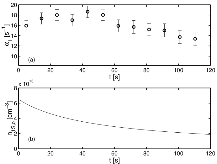
Figure 12: (a) Weighted average of $\alpha_{1}$ determined by extrapolation to zero metastable signal in Trap W as a function of time after sample preparation. Each point represents a value of $\alpha_{1}$ extracted from 9.6 s of $2S$ decay data. The one-body metastable loss rate appears to decrease as the ground state sample decays, suggesting that some of the one-body loss may be due to $1S$-$2S$ inelastic collisions. The bottom of the plot corresponds to the natural decay rate, and error bars include only statistical uncertainties. (b) Peak ground state density calculated as a function of time in Trap W assuming that the only significant $1S$ loss mechanism is dipolar decay.

By dividing the decay data for a single trap into time bins corresponding to a fixed number of sweeps across resonance, we can examine whether the one-body loss rate changes as the ground state sample decays at a constant temperature. Figure 12(a) shows values for $\alpha_{1}$ determined in consecutive time bins for Trap W. The putative ground state density is shown for the same time interval in Fig. 12(b). Although not conclusive, the data suggests that the total one-body loss rate decreases as the $1S$ density decreases. This decrease in $\alpha_{1}$ may be due to a decline in inelastic $1S$-$2S$ collision rates, which are proportional to the ground state density. In principle, the points of Fig. 12(a) could be fit to a model which includes constant one-body decay terms and a term proportional to the $1S$ density. The uncertainties in both the determinations of $\alpha_{1}$ and the density as a function of time are too large, however, to extract a meaningful value for the total $1S$-$2S$ inelastic loss rate without prior knowledge of the stray electric field contribution.

On the other hand, it is possible to establish a conservative upper limit on the total inelastic contribution $\alpha_{1,{\rm inel}}$ to the one-body decay rate by subtracting the natural decay rate from $\alpha_{1}$:

$$\alpha_{1,{\rm inel}}<\alpha_{1}-\gamma_{\rm nat}.$$ (23)

In the static approximation, $\alpha_{1,{\rm inel}}$ can be simply related to the total metastable loss rate constant for inelastic $1S$-$2S$ collisions $K_{12}$, defined by

$$\Bigl{.}\dot{n}_{2S}({\bf r})\Bigr{|}_{1S-2S}=-K_{12}\,n_{1S}({\bf r})n_{2S}({\bf r}).$$ (24)

Note that $K_{12}$ only encompasses collisions resulting in loss of a $2S$ atom from the trap; for example, collisions in which only the $1S$ atom changes state are not included. Integrating both sides of Eq. 24 over all space, we obtain

$$\Bigl{.}\dot{N}_{2S}\Bigr{|}_{1S-2S} = -K_{12}\int n_{1S}({\bf r})n_{2S}({\bf r})\,d^{3}{\bf r}$$ (25)

$$= -K_{12}n_{1S,o}n_{2S,o}\int f_{1S}({\bf r})f_{2S}({\bf r})\,d^{3}{\bf r}$$ (26)

$$= -\left(\frac{K_{12}n_{1S,o}Q_{12}}{V_{2S}}\right)N_{2S},$$ (27)

where $Q_{12}=\int f_{1S}({\bf r})f_{2S}({\bf r})\,d^{3}{\bf r}$ is an overlap integral for the ground state and metastable clouds. Since by definition

$$\Bigl{.}\dot{N}_{2S}\Bigr{|}_{1S-2S}=-\alpha_{1,{\rm inel}}N_{2S},$$ (28)

it immediately follows that

$$K_{12}=\frac{\alpha_{1,{\rm inel}}V_{2S}}{n_{1S,o}Q_{12}}.$$ (29)

By combining an upper limit for the initial value of $\alpha_{1,{\rm inel}}$ in a trap with an upper limit for the ratio $V_{2S}/Q_{12}$ and the known peak density $n_{1S,o}$, an upper limit for $K_{12}$ is obtained. An upper limit for $\alpha_{1,{\rm inel}}$ has been estimated for each trap by first fitting a line to $\alpha_{1}$ as a function of time and then subtracting $\gamma_{\rm nat}$ from the initial value of the fitted line. In Trap W, for example, the data suggests that $\alpha_{1}$ may be as large as 18 s^-1, implying an upper limit of 10 s^-1 for $\alpha_{1,{\rm inel}}$. The ratio $V_{2S}/Q_{12}$ can be computed numerically using the Monte Carlo $2S$ distribution results; it has a maximum value of approximately 3 for all traps with all probable excitation geometries. Upper limits for $K_{12}$ are summarized in Table 6.

The experimental upper limits for $K_{12}$ are more than two orders of magnitude larger than the rate constant $g=1.2\times 10^{-15}$ cm³/s for $1S$-$1S$ dipolar decay. If the true value of $K_{12}$ turns out to be closer to the upper limits in Table 6 than to $g$ in this temperature range, this may imply that $1S$-$2S$ excitation transfer collisions (Eq. 14) are much more likely than $1S$-$2S$ hyperfine-changing collisions (Eq. 13) mediated by magnetic dipole forces. More precise metastable decay measurements are required to establish lower bounds for $K_{12}$.

Trap	$T$ (mK)	$K_{12}$ $(10^{-13}$ cm3/s)
W	0.087	$<5$
X	0.23	$<3$
Y	0.45	$<2$
Z	2.3	$<11$

Table 6: Experimental upper limits for $K_{12}$ in the static approximation.

Chapter 5 Outlook: Spectroscopy of Metastable Hydrogen

As mentioned in the introduction to this thesis, the ability to produce large, long-lived clouds of metastable H in a magnetic trap opens the door for a variety of new experiments involving excited states of hydrogen. Of particular interest are spectroscopic experiments involving transitions from the $2S$ state to higher-lying states (Fig. 1). Spectroscopy of a strong single-photon transition such as the $2S$-$3P$ Balmer-$\alpha$ transition will provide a more sensitive probe of the metastable cloud. Excitation on this transition may also allow the first direct imaging of the metastable cloud. From a fundamental physics standpoint, the most exciting possibilities of all involve precision spectroscopy of two-photon $2S$-$nS$ transitions [21]. Recent breakthroughs in optical frequency metrology [18] make it more feasible than ever to measure these frequencies with unprecedented accuracy, leading to improved values for the Lamb shift and Rydberg constant [12].

This chapter contains a brief discussion of experiments which could feasibly be carried out in the next few years. Much fruitful work can be done yet with the current cryogenic apparatus. However, to fully exploit the promise of metastable H spectroscopy, a new apparatus with more optical access and better detection efficiency is desired.

Figure 1: Some transitions from the metastable state of hydrogen which can be excited with readily available diode lasers. Spectroscopy of these transitions in trapped metastable hydrogen may provide new insight into cold collisions and also fundamental physics.

1 Further Experiments with the Current Apparatus

1 Optical Refinements

The principal sources of systematic noise and uncertainty for experiments with metastables are currently related to the UV excitation laser. There are a number of possible refinements to the optical apparatus which would dramatically reduce these systematics.

In the determination of $K_{2}$ described in Ch. 4, a major source of uncertainty stemmed from uncertainty in the overlap of the laser focuses along the trap axis. This overlap can be done empirically by changing the length of the telescope nearest the cryostat (see Fig. 8) and observing the change in metastable signal. Assuming the centroid of the laser focuses is near the bottom of the trap in $z$, the signal will be optimized when the focuses are overlapped. To perform this optimization accurately, the telescope length should be scanned during a single trap cycle with stable UV power. This could be accomplished by mounting one of the telescope lenses on a computer-controlled stepper motor. Another source of uncertainty is the spot size at the laser focuses. It is difficult to measure the beam radius at the UV waists directly, but the radius could be inferred more accurately by measuring the beam profile at several points outside of the cryostat.

On a time scale of seconds to minutes, fluctuations in the transverse overlap of the laser focuses is probably the most important source of non-statistical noise in our $1S$-$2S$ spectroscopy. Some of this noise is apparently due to the pendulum motion of the 2.5 m-long cryostat. Greater efforts to mechanically isolate the cryostat from low frequencies may alleviate this problem. Improving the pointing and transverse mode stability of the UV beam will also make the task of actively stabilizing the beam overlap in the cryostat much easier. Currently, much of the noise in the UV beam pointing and mode quality is due to the instability of the 486 nm dye laser beam which pumps the SHG cavity (Fig. 8). The pointing and mode stability of the dye laser output could be greatly enhanced by spatial filtering, such as by passing the the beam through a short length of fiber. This would come at the expense of a significant amount of power, but the trade-off of power for stability may be worthwhile for some experiments.

With a more stable UV laser and less uncertainty in the laser geometry, the decay measurements described in this thesis could be performed with a better signal-to-noise ratio, and interpretation of the data would be more straightforward. In general, the geometry of the metastable cloud could be predicted more accurately, thus reducing a major uncertainty in the measurement of $K_{2}$. Another important source of uncertainty, the calibration of the detection efficiency, would also benefit from a better-known and more stable laser geometry. However, it may be difficult to significantly improve the measurement of $K_{2}$ or other collisional parameters without a new method for metastable detection. One possibility is Balmer-$\alpha$ spectroscopy, discussed below in Sec. 3.

2 Excitation Studies

Information about photoionization and two-body loss can be gleaned from studies of the number of metastables excited as a function of the excitation pulse length. Results from a preliminary study of this type can be seen in Fig. 2. The number of $2S$ atoms generated begins to saturate after a few milliseconds. This is consistent with simulations of excitation behavior which incorporate the theoretical value for the photoionization cross-section at 243 nm. In cold, dense samples, $2S$-$2S$ two-body loss can play an important role in the saturation behavior as well.

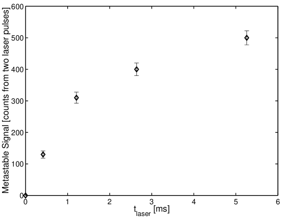
Figure 2: Metastable signal observed for different excitation pulse lengths when quenching at a fixed wait time of 5 ms after the excitation pulse. The sample was prepared at roughly 200 $\mu$K in a magnetic trap similar to Trap W, and the laser was tuned to the peak of the Doppler-free $1S$-$2S$ line. The number of metastables begins to saturate at long pulse times due to photoionization and two-body loss.

Each point in Fig. 2 was measured in a different trap cycle. The duty cycle of the mechanical beam chopper and the timing generator were adjusted between cycles to produce different excitation pulse lengths with a constant wait time between the end of the excitation pulse and the quench pulse. Such a study requires a couple hours to execute and is sensitive to drift in mode quality, power, and alignment of the UV beam over this time scale. A better way to look at the excitation behavior of metastables would be to use different excitation pulse lengths in succession during a single trap cycle. This could be accomplished using a fast mechanical shutter or a chopper wheel with several different-sized apertures. An AOM could also be used to chop the beam at the expense of about 40% of the UV power.

Experimental excitation curves measured in different traps could be analyzed with a numerical model incorporating excitation, photoionization, and collisional loss mechanisms. In traps where the metastable density is low enough so that two-body loss is not important, photoionization will be the principal loss mechanism at high UV powers. If geometry and laser power are well known, the data could be analyzed to verify the photoionization cross section. Alternatively, it may be possible to use the theoretical cross section to calibrate the laser intensity. Finally, in situations where the metastable density is very large, it may be possible to correct the saturation curve for photoionization and extract a two-body loss rate. Excitation studies may serve as a useful complement to the decay measurements described in this thesis.

3 Balmer-$\alpha$ Spectroscopy

Preliminary work has been completed in the MIT Ultracold Hydrogen Group towards probing the $2S$-$3P$ transition with a 656 nm diode laser. The retromirror of the current trapping cell has a dichroic dieletric coating which is 99% reflective at both 243 nm and 656 nm. Thus, red Balmer-$\alpha$ light can be introduced into the cryostat along the same path as the UV beam, and the retro-reflected red light can be detected using a beam splitter outside the cryostat. This is potentially a highly sensitive probe of the metastable cloud. Alternatively, the absorption of red light can be surmised from the depletion of the metastable number, observed by quenching and detecting Lyman-$\alpha$ as before.

Diode lasers with free-running wavelengths near 656 nm and output powers up to 50 mW are commercially available for $\sim\$100$. The diodes can be induced to operate at a single frequency in a single transverse mode by optical feedback from an external grating. The laser frequency can be actively stabilized by piezoelectric control of the grating angle. With a standard external-cavity grating-stabilized diode laser design, a linewidth of a few hundred kilohertz is easily achieved [78, 79]. For Balmer-$\alpha$ spectroscopy, it is convenient to use the $2S$-$3P$ saturated absorption lines of a hydrogen discharge as the frequency reference. The stabilized laser linewidth is small compared to the 30 MHz natural linewidth of the Balmer-$\alpha$ transition. At 100 $\mu$K, the Doppler width is only about 10% of the natural linewidth, and Zeeman broadening will be insignificant. Thus, in experiments with trapped metastables, the experimental Balmer-$\alpha$ linewidth will be approximately the natural linewidth.

The Einstein coefficients relevant for atoms in the $3P$ state are $A_{3P-1S}=1.64\times 10^{8}$ s^-1 and $A_{3P-2S}=0.22\times 10^{8}$ s^-1 [80]. The excitation rate $W_{2S-3P}$ from $2S$ to $3P$ in the presence of a resonant 656 nm laser can be written

$$W_{2S-3P}=\sigma_{o}\left(\frac{I}{\hbar\omega}\right)$$ (1)

where $I$ is the intensity and the resonant absorption cross-section is

$$\sigma_{o}=\left(\frac{A_{3P-2S}}{A_{3P-1S}+A_{3P-2S}}\right)6\pi\left(\frac{\lambda}{2\pi}\right)^{2}=2.4\times 10^{-10}\,{\rm cm}^{2}.$$ (2)

For absorption experiments, the Balmer-$\alpha$ beam waist should be larger than the thermal radius of the metastable cloud. This will facilitate alignment and allow saturation intensity to be achieved over most of the atom cloud with a modest laser power. Consider, for example, a metastable cloud in Trap W, which has a thermal radius of approximately 110 $\mu$m. If the laser radius is three times larger, then the minimum power required for saturation at the center of the trap is 24 $\mu$W. In an absorption experiment, the Balmer-$\alpha$ laser would be pulsed at a tiny duty cycle, and even at powers far above saturation, the heating of the trapping cell and cryostat would be negligible.

It should be possible to make absorption measurements which are nearly shot noise limited. To minimize shot noise, laser pulses can be used which contain only as many photons as are necessary to excite most of the metastables. For the case of a saturation power beam with radius three times larger than the thermal radius in Trap W, a $\sim 200$ ns pulse of $\sim 10^{7}$ photons can excite most of a cloud of $10^{7}$ metastable atoms to the $3P$ state. The relative error due to shot noise for each laser pulse will only be $\sim 10^{-7/2}$, which is less than 0.1%. In practice, it will be more convenient to use somewhat longer laser pulses and lower power, but similar shot noise levels should be achievable. This shot noise limit would be a dramatic improvement from the $\sim 10$% statistical error on the $\sim 100$ Lyman-$\alpha$ photons observed after a typical quench pulse.

By calibrating the number of photons removed from the Balmer-$\alpha$ beam, it will be possible to measure the number of metastables in the trap. This may lead to a better calibration of the detection efficiency for metastables by the quenching method. The relative attenuation of the 656 nm beam will additionally give the column density of the metastable cloud. Used in combination with the shape of the magnetic trap, this data may allow a better determination of the spatial distribution of metastables. Spectroscopy of the Balmer-$\alpha$ line may also provide information about the temperature of the sample. For an accurate temperature determination, the signal-to-noise ratio will have to be high, since the Doppler broadening of typical samples is much smaller than the natural $2S$-$3P$ linewidth. Other experiments, such as photoassociation spectroscopy on the $2S$-$3P$ transition may become possible as well.

In the long term, imaging of the metastable cloud using Balmer-$\alpha$ fluorescence may be the most useful diagnostic of all for trapped metastable hydrogen. The implementation of an imaging detector, however, will require major changes to the apparatus (Sec. 2).

4 Precision Spectroscopy and Frequency Metrology

In the introduction to this thesis, it was described how the measurement of a $2S$-$nS$ frequency interval, when combined with the accurately known $1S$-$2S$ frequency, allows various contributions to the structure of the hydrogen atom to be deconvolved. With a sample of cold metastable hydrogen, it should be possible to improve the accuracy of $2S$-$nS$ frequencies by an order of magnitude over the best measurements to date. This will lead to a corresponding increase in the accuracy of the Rydberg constant and Lamb shift. If the frequencies of several $2S$-$nS$ transitions can be measured precisely, we will have stringent checks on the understanding of systematic effects.

As a first demonstration of two-photon metastable H spectroscopy, the MIT Ultracold Hydrogen Group plans to use light from a 972 nm diode laser to excite the the $2S$-$4S$ transition. To perform Doppler-free two-photon spectroscopy, a standing wave is required, and most likely the current retromirror will have to be replaced with one designed for higher reflectivity at 972 nm. The diode laser technology for this and other $2S$-$nS$ transitions is similar to what was described above for the Balmer-$\alpha$ frequency. The $2S$-$4S$ interval differs by less than 5 GHz from $1/4$ of the $1S$-$2S$ interval; frequency metrology can be accomplished by looking at the beat note between the 486 nm dye laser, which is frequency-doubled to excite the $1S$-$2S$ transition, and the second harmonic of the 972 nm laser. Because it has been calibrated precisely against a cesium standard, the $1S$-$2S$ transition serves as a de facto secondary frequency standard [13].

Stimulated by our need for convenient optical frequency metrology, a new mode-locked femtosecond laser has recently been developed in the group of F. Kärtner at MIT [81, 82]. The “double-chirped” mirrors of this laser allow it to produce an extraordinarily broad comb of frequencies without dispersion-compensating prisms or fiber. It will allow direct comparison of optical frequencies in the range 600-1100 nm. Likely candidates for precision spectroscopy are the $2S$-$8S$ (two photons at 778 nm) and $2S$-$10S$ (two photons at 759 nm) transitions, whose frequencies have been measured previously in beam experiments. In an experiment with cold metastable hydrogen, these frequencies could be calibrated with the frequency comb and the 972 nm subharmonic of the $1S$-$2S$ transition. An alternative approach is to frequency-triple part of the comb for direct comparison with the 243 nm frequency.

Based on our studies with metastable hydrogen so far, we can speculate that the optimum metastable cloud for $2S$-$nS$ spectroscopy in the current apparatus will be similar to the one excited in Trap X (Sec. 1). In this sample, the peak $2S$ density $(>3\times 10^{10}$ cm${}^{-3})$ and number $(>4\times 10^{7})$ are sufficient to allow high $2S$-$nS$ excitation rates. At the same time, two-body loss will not play a significant role in limiting the signal rate; $K_{2}$ appears to be roughly a factor of 2 smaller at 230 $\mu$K as compared to 90 $\mu$K (Fig. 11), and the metastable density is somewhat smaller in the warmer trap as well. The moderate ground state density in Trap X may also be desired to reduce the complicating effects of cold collision shifts and inelastic collisions involving $1S$ atoms.

Before concluding this section, it is worth mentioning that the mode-locked femtosecond laser will also permit a new determination of the $1S$-$2S$ absolute frequency. Using an appropriate optical frequency divider [11], two optical frequencies with an interval having a simple relationship to the $1S$-$2S$ frequency can be produced inside the range of the mode-locked laser’s frequency comb. With the apparatus changes described in the next section, it should be possible to perform $1S$-$2S$ spectroscopy with much lower ground state densities, minimizing the cold collision shift, which is currently the most source of important systematic error. Provided a primary reference such as a cesium fountain clock, the transition frequency can potentially be measured with an accuracy surpassing that of Hänsch and collaborators [13].

2 A Cryogenic Trap Optimized for Optical Studies

A redesign of the magnet system and cryostat to improve optical access and detection solid angle will have many benefits for spectroscopic and other optical studies of trapped hydrogen. These include better signal-to-noise ratios, easier alignment, more possible geometries for probe beams, and the potential to use imaging detectors.

Figure 3 is a schematic for a possible cryostat and magnet system with a geometry favorable for optical experiments. The cross section shows eight superconducting “Ioffe bars” which give rise to a radial quadrupole field. “Pinch” solenoids above and below the plane of the page would provide the axial confinement. Spaces between the Ioffe bars provide access for laser beams and detectors. As in the current apparatus, an additional window on the axis of the trap could allow entry of a retro-reflected 243 nm beam for generation of metastables.

The cryogenic apparatus can be greatly simplified if we sacrifice the ability to do rf evaporation. Our experiments have shown that large numbers and high densities of metastables can be produced without rf evaporation of the ground state sample (as in Trap X, for example). In Fig. 3, the trapping cell could be made from a tube of non-magnetic metal with high thermal conductivity, such as copper. To incorporate four windows as shown, a square profile may be most convenient. Even more complexity can be avoided if the cryostat is based on a ³He refrigerator rather than a dilution refrigerator. The lowest practical temperature of a ³He refrigerator is about 300 mK, which in the present loading scheme is too warm for the atom cloud to thermally disconnect from the cell walls (Sec. 4). It may be possible, however, to induce thermal disconnect by raising the magnetic fields at the walls and forcing magnetic saddlepoint evaporation elsewhere.

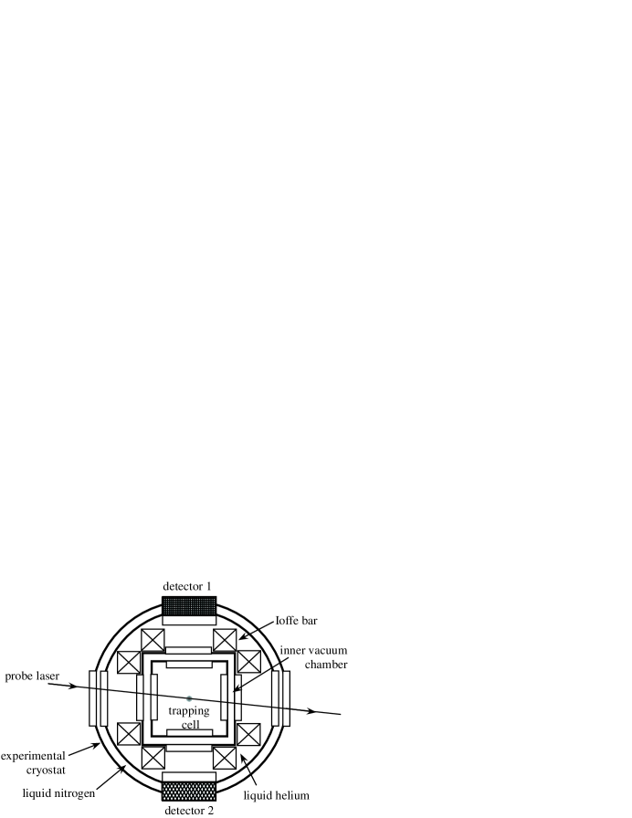
Figure 3: Cross-sectional view of cryogenic trapping apparatus with transverse optical access and large detection solid angle. Metastable hydrogen could be excited, as done currently, by a 243 nm laser along the axis of the Ioffe-Pritchard trap (oriented into the page at the center of the trapping cell). One or more probe lasers could be introduced transverse to the atom cloud. Each of the detectors, anchored at liquid nitrogen temperature, could be a CCD, PMT array, or MCP detector. The magnet system and detector mounts must be designed so that magnetic fields are compatible with the detectors.

It is desirable to reduce both the aspect ratio of the trap and the length of the axial dimension of the entire apparatus. With more axial compression, the atom clouds would be more easily probed with transverse laser beams, and the efficiency of magnetic saddlepoint evaporation at low temperatures may be enhanced [83]. If the length of the whole apparatus can be significantly reduced, this will facilitate reduction of fluctuations in the transverse overlap of the UV beams, currently a major source of noise in our experiments. With a ³He refrigerator, it may even be possible to mount the entire cryostat on an optical table.

Bringing the detectors close to the atoms and providing them with a large numerical aperture will greatly enhance the detection efficiency. Fig. 3 depicts an arrangement where the detectors sit in contact with a liquid nitrogen jacket and can be easily swapped out, depending on the experiments being performed. With a large detection solid angle, it should be possible to observe the natural two-photon fluorescence decay of metastables without applying a quench pulse. With Lyman-$\alpha$ detectors, the fluorescence occurring due to excitation transfer can be observed during the decay of the metastable cloud; the relative importance of ionization and excitation transfer processes could be unraveled. With a CCD camera and a Balmer-$\alpha$ source, the metastable cloud can be imaged as in most other atom trapping experiments. This diagnostic would potentially yield a wealth of information about the $2S$ and, indirectly, the $1S$ samples.

With a much improved detection efficiency, it will be possible to do spectroscopy with significantly lower laser powers or significantly lower ground state densities than at present. If lower laser powers are possible, then the UV retromirror could exist outside of the cryostat, and it could be either vibrationally isolated or actively stabilized to ensure a stable overlap of the counterpropagating beams. Lower $1S$ densities are key for minimizing cold collision shifts. In particular, the combination of high detection efficiency and low sample density is desired for pushing spectroscopy of the $1S$-$2S$ transition to unprecedented resolution levels.

For spectroscopy of the metastable cloud, the benefits of close optical access to the atoms on two sides are clear. The necessary beams would be easy to introduce and align. For one-photon transitions like $2S$-$3P$, single-pass absorption experiments would be possible. For the the two-photon $2S$-$nS$ transitions, the retromirror needed to achieve a standing wave could be positioned outside the cryostat.

The possibilities for the next generation spectroscopy apparatus are so many, it may be difficult to choose which ones to pursue. We can be certain, however, that metastable H has many stories yet to tell us about cold collisions and fundamental physics.

References

- [1] T. C. Killian. 1S-2S Spectroscopy of Trapped Hydrogen: The Cold Collision Frequency Shift and Studies of BEC. PhD thesis, Massachusetts Institute of Technology, 1999.
- [2] Thomas C. Killian, Dale G. Fried, Lorenz Willmann, David Landhuis, Stephen C. Moss, Daniel Kleppner, and Thomas J. Greytak. Cold-collision frequency shift of the - transition in hydrogen. Physical Review Letters, 81:3807, 1998.
- [3] M. J. Jamieson, A. Dalgarno, and J. M. Doyle. Scattering lengths for collisions of ground state and metastable state hydrogen atoms. Molecular Physics, 87:817, 1996.
- [4] T. Orlikowski, G. Staszewska, and L. Wolniewicz. Long range adiabatic potentials and scattering lengths for the EF, e and h states of the hydrogen molecule. Molecular Physics, 96:1445, 1999.
- [5] C. J. Pethick and H. T. C. Stoof. Collisional frequency shifts of absorption lines in an atomic hydrogen gas. Physical Review A, 64:013618, 2001.
- [6] X. Urbain, A. Cornet, and J. Jureta. Associative ionization in collisions between metastable hydrogen atoms. Journal of Physics B: Atomic, Molecular, and Optical Phyics, 25:L189, 1992.
- [7] R. C. Forrey, S. Jonsell, P. Froelich, A. Saenz, and A. Dalgarno, to be published.
- [8] D. Landhuis, L. Matos, S. C. Moss, K. Vant, J. K. Steinberger, L. Willmann, T. J. Greytak, and D. Kleppner, in preparation.
- [9] R. C. Forrey, R. Côté, A. Dalgarno, S. Jonsell, A. Saenz, and P. Froelich. Collisions between metastable hydrogen atoms at thermal energies. Physical Review Letters, 85:4245, 2000.
- [10] N. Balakrishnan, R. C. Forrey, and A. Dalgarno. Quenching of H2 vibrations in ultracold 3He and 4He collisions. Physical Review Letters, 80:3224, 1998.
- [11] Th. Udem, A. Huber, B. Gross, J. Reichert, M. Prevedelli, M. Weitz, and T. W. Hänsch. Phase-coherent measurement of the hydrogen - transition frequency with an optical frequency interval divider chain. Physical Review Letters, 79:2646, 1997.
- [12] C. Schwob, L. Jozefowski, B. de Beauvoir, L. Hilico, F. Nez, L. Julien, F. Biraben, O. Acef, J.-J. Zondy, and A. Clairon. Optical frequency measurement of the - transitions in hydrogen and deuterium: Rydberg constant and Lamb shift determinations. Physical Review Letters, 82:4960, 1999.
- [13] M. Niering, R. Holzwarth, J. Reichert, P. Pokasov, Th. Udem, M. Weitz, T. W. Hänsch, P. Lemonde, G. Santarelli, M. Abgrall, P. Laurent, C. Salomon, and A. Clairon. Measurement of the hydrogen - transition frequency by phase coherent comparison with a microwave cesium fountain clock. Physical Review Letters, 84:5496, 2000.
- [14] K. Pachucki. Logarithmic two-loop corrections to the Lamb shift in hydrogen. Physical Review A, 63:042503–1, 2001.
- [15] M. Weitz, A. Huber, F. Schmidt-Kaler, D. Leibfried, W. Vassen, C. Zimmermann, K. Pachucki, T. W. Hänsch, L. Julien, and F. Biraben. Precision measurement of the ground-state Lamb shift in atomic hydrogen and deuterium by frequency comparison. Physical Review A, 52:2664, 1995.
- [16] S. Bourzeix, B. de Beauvoir, F. Nez, M. D. Plimmer, F. de Tomasi, L. Julien, F. Biraben, and D. N. Stacy. High resolution spectroscopy of the hydrogen atom: determination of the Lamb shift. Physical Review Letters, 76:384, 1996.
- [17] B. de Beauvoir, F. Nez, L. Julien, B. Cagnac, F. Biraben, D. Touahri, L. Hilico, O. Acef, A. Clairon, and J. J. Zondy. Absolute freqeuncy measurement of the - transitions in hydrogen and deuterium: New determination of the Rydberg constant. Physical Review Letters, 78:440, 1997.
- [18] Th. Udem, J. Reichert, R. Holzwarth, and T. W. Hänsch. Accurate measurement of large optical frequency differences with a mode-locked laser. Optics Letters, 24:881, 1999.
- [19] S. A. Diddams, D. J. Jones, J. Ye, S. T. Cundiff, J. L. Hall, J. K. Ranka, R. S. Windeler, R. Holzwarth, Th. Udem, and T. W. Hänsch. Direct link between microwave and optical frequencies with a 300 THz femtosecond laser comb. Physical Review Letters, 84:5102, 2000.
- [20] Th. Udem, S. A. Diddams, K. R. Vogel, C. W. Oates, E. A. Curtis, W. D. Lee, W. M. Itano, R. E. Drullinger, J. C. Bergquist, and L. Hollberg. Absolute frequency measurements of Hg+ and Ca optical clock transitions with a femtosecond laser. Physical Review Letters, 86:4996, 2001.
- [21] L. Willmann and D. Kleppner. Ultracold hydrogen. In S. G. Karshenboim, F. S. Pavone, F. Bassani, M. Inguscio, and T. W. Hänsch, editors, The Hydrogen Atom: Precision Physics of Simple Atomic Systems, pages 42–56. Springer-Verlag, 2001.
- [22] M. Yasuda and F. Shimizu. Observation of two-atom correlation of an ultracold neon atomic beam. Physical Review Letters, 77:3090, 1996.
- [23] M. Morinaga, M. Yasuda, T. Kishimoto, F. Shimizu, J. Fujita, and S. Matsui. Holographic manipulation of a cold atomic beam. Physical Review Letters, 77:802, 1996.
- [24] A. Robert, O. Sirjean, A. Browaeys, J. Poupard, S. Nowak, D. Boiron, C. I. Westbrook, and A. Aspect. A Bose-Einstein condensate of metastable atoms. Science, 292:461, 2001.
- [25] M. Kozuma, L. Deng, E. W. Hagley, J. Wen, R. Lutwak, K. Helmerson, S. L. Rolston, and W. D. Phillips. Coherent splitting of Bose-Einstein condensed atoms with optically induced Bragg diffraction. Physical Review Letters, 82:871–875, 1999.
- [26] S. Nowak, T. Pfau, and J. Mlynek. Nanolithography with metastable helium. Applied Physics B, 63:203, 1996.
- [27] K. S. Johnson, J. H. Thywissen, N. H. Dekker, K. K. Berggren, A. P. Chu, R. Younkin, and M. Prentiss. Localization of metastable atom beams with optical standing waves: Nanolithography at the Heisenberg limit. Science, 280:1583, 1998.
- [28] H. F. Hess, G. P. Kochanski, J. M. Doyle, N. Masuhara, D. Kleppner, and T. J. Greytak. Magnetic trapping of spin-polarized atomic hydrogen. Physical Review Letters, 59:672, 1987.
- [29] J. M. Doyle. Energy Distribution Measurements of Magnetically Trapped Spin Polarized Atomic Hydrogen: Evaporative Cooling and Surface Sticking. PhD thesis, Massachusetts Institute of Technology, 1991.
- [30] C. L. Cesar, D. G. Fried, T. C. Killian, A. D. Polcyn, J. C. Sandberg, I. A. Yu, T. J. Greytak, D. Kleppner, and J. M. Doyle. Two-photon spectroscopy of trapped atomic hydrogen. Physical Review Letters, 77:255, 1996.
- [31] H. A. Bethe and E. E. Salpeter. Quantum Mechanics of One- and Two-Electron Atoms, page 214. Plenum Publishing Corp., 1977.
- [32] D. E. Pritchard. Cooling neutral atoms in a magnetic trap for precision spectroscopy. Physical Review Letters, 51:1336, 1983.
- [33] F. Biraben, M. Bassini, and B. Cagnac. Line-shapes in Doppler-free two-photon spectroscopy. The effect of finite transit time. Le Journal de Physique, 40:445, 1979.
- [34] Dale G. Fried, Thomas C. Killian, Lorenz Willmann, David Landhuis, Stephen C. Moss, Daniel Kleppner, and Thomas J. Greytak. Bose-Einstein condensation of atomic hydrogen. Physical Review Letters, 81:3811, 1998.
- [35] R. G. Beausoleil. Continuous-Wave Measurement of the 1S-2S Transition Frequency in Atomic Hydrogen: The 1S Lamb Shift. PhD thesis, Stanford University, 1986.
- [36] J. C. Sandberg. Research Toward Laser Spectroscopy of Trapped Atomic Hydrogen. PhD thesis, Massachusetts Institute of Technology, 1993.
- [37] C. L. Cesar and D. Kleppner. Two-photon Doppler-free spectroscopy of trapped atoms. Physical Review A, 59:4564, 1999.
- [38] C. L. Cesar. Two-Photon Spectroscopy of Trapped Atomic Hydrogen. PhD thesis, Massachusetts Institute of Technology, 1995.
- [39] D. G. Fried. Bose-Einstein Condensation of Atomic Hydrogen. PhD thesis, Massachusetts Institute of Technology, 1999.
- [40] H. T. C. Stoof, J. M. V. A. Koelman, and B. J. Verhaar. Spin-exchange and dipole relaxation rates in atomic hydrogen: Rigorous and simplified calculations. Physical Review B, 38:4688, 1988.
- [41] E. A. Cornell, J. R. Ensher, and C. E. Wieman. Experiments in dilute atomic Bose-Einstein condensates. In M. Inguscio, et al., editor, Bose-Einstein Condensation in Atomic Gases. Proceedings of the International School of Physics “Enrico Fermi”, Course CXL, IOS Press Ohmsha, 1999.
- [42] K. Dieckmann. Bose-Einstein Condensation with High Atom Number in a Deep Magnetic Trap. PhD thesis, University of Amsterdam, 2001.
- [43] S. C. Moss. Formation and Decay of a Bose-Einstein Condensate in Atomic Hydrogen. PhD thesis, Massachusetts Institute of Technology, 2002.
- [44] I. A. Yu. Ultracold Surface Collisions: Sticking Probability of Atomic Hydrogen on Superfluid 4He. PhD thesis, Massachusetts Institute of Technology, 1993.
- [45] Valpey Fisher Corporation.
- [46] Emerson & Cumming Inc., Canton, Massachusetts.
- [47] Acheson Colloids Company, Port Huron, Michigan.
- [48] J. M. Greben, A. W. Thomas, and A. J. Berlinsky. Quantum theory of hydrogen recombination. Canadian Journal of Physics, 59:945, 1981.
- [49] H. T. C. Stoof, private communication.
- [50] T. J. Greytak, unpublished.
- [51] O. J. Luiten, M. W. Reynolds, and J. T. M. Walraven. Kinetic theory of evaporative cooling of a trapped gas. Physical Review A, 53:381, 1996.
- [52] D. A. Bell, H. F. Hess, G. P. Kochanski, S. Buchman, L. Pollack, Y. M. Xiao, D. Kleppner, and T. J. Greytak. Relaxation and recombination in spin-polarized atomic hydrogen. Physical Review B, 34:7670, 1986.
- [53] A. I. Safonov, S. A. Vasilyev, A. A. Kharitonov, I. I. Lukashevich S. T. Boldarev, and S. Jaakola. Adsorption and two-body recombination of atomic hydrogen on 3He-4He mixture films. Physical Review Letters, 86:15, 2001.
- [54] R. Kallenbach, C. Zimmermann, D. H. McIntyre, and T.W. Hänsch. A blue dye laser with sub-kilohertz stability. Optics Communications, 70:56, 1989.
- [55] Coherent Laser Group, Santa Clara, California.
- [56] Radiant Dyes GmbH, Wermelskirchen, Germany.
- [57] R. W. P. Drever, J. L. Hall, F. V. Kowalski, J. Hough, G. M. Ford, A. J. Munley, and H. Ward. Laser phase and frequency stabilization using an optical resonator. Applied Physics B, 31:97, 1983.
- [58] D. H. McIntyre. High Resolution Laser Spectroscopy of Tellurium and Hydrogen: A Measurement of the Rydberg Constant. PhD thesis, Stanford University, 1987.
- [59] T. W. Hänsch and B. Couillaud. Laser frequency stabilization by polarization spectroscopy of a reflecting reference cavity. Optics Communications, 35:441, 1980.
- [60] Part number AE0203D04, Thorlabs, Inc., Newton, New Jersey.
- [61] H. A. Bethe and E. E. Salpeter. Quantum Mechanics of One- and Two-Electron Atoms, page 287. Plenum Publishing Corp., 1977.
- [62] S. Jonsell, A. Saenz, P. Froelich, R. C. Forrey, R. Côté, and A. Dalgarno. Long-range interactions between two excited hydrogen atoms. Physical Review A, 65:042501, 2002.
- [63] R. C. Forrey, private communication.
- [64] R. van Roijen, J. J. Berkhout, S. Jaakkola, and J. T. M. Walraven. Experiments with atomic hydrogen in a magnetic trapping field. Physical Review Letters, 61:931, 1988.
- [65] E. P. Wigner. On the behavior of cross sections near thresholds. Physical Review, 73:1002, 1948.
- [66] J. Weiner, V. S. Bagnato, S. Zilio, and P. S. Julienne. Experiments and theory in cold and ultracold collisions. Reviews of Modern Physics, 71:1, 1999.
- [67] L. Wolniewicz, private communication.
- [68] M. J. Jamieson, A. Dalgarno, and M. Kimura. Scattering lengths and effective ranges for He-He and spin-polarized H-H and D-D scattering. Physical Review A, 51:2626, 1995.
- [69] M. Ö. Oktel, T. C. Killian, D. Kleppner, and L. S. Levitov. Sum rule for the optical spectrum of a trapped gas. Physical Review A, 65:033617, 2002.
- [70] S. C. Moss, D. Landhuis, L. Matos, K. Vant, J. K. Steinberger, L. Willmann, T. J. Greytak, and D. Kleppner, in preparation.
- [71] A. Burgess. Tables of hydrogenic photoionization cross-sections and recombinations coefficients. Memoirs of the Royal Astronomical Society, 69:1, 1965.
- [72] J. J. Sakurai. Modern Quantum Mechanics, pages 339–341. Addison-Wesley, revised edition, 1994.
- [73] D. W. Snoke and J. P. Wolf. Population dynamics of a Bose gas near saturation. Physical Review B, 39:4030, 1989.
- [74] J. F. O’Hanlon. A User’s Guide to Vacuum Technology, page 20. Wiley, 2nd edition, 1989.
- [75] S. Chapman and T. G. Cowling. The Mathematical Theory of Non-Uniform Gases, page 195. Cambridge U. P., 3rd edition, 1970.
- [76] A. Dalgarno, private communication.
- [77] B. H. Bransden and C. J. Joachain. Physics of Atoms and Molecules, pages 212–214. Longman, 1983.
- [78] C. E. Wieman and L. Hollberg. Using diode lasers for atomic physics. Review of Scientific Instruments, 62:1, 1991.
- [79] K. B. MacAdam, A. Steinbach, and C. Wieman. A narrow-band tunable diode laser system with grating feedback, and a saturated absorption spectrometer for Cs and Rb. American Journal of Physics, 60:1098, 1992.
- [80] H. A. Bethe and E. E. Salpeter. Quantum Mechanics of One- and Two-Electron Atoms, page 266. Springer-Verlag, 1957.
- [81] T. R. Schibli, L. M. Matos, F. J. Grawert, J. G. Fujimoto, and F. X. Kärtner, in preparation.
- [82] R. Ell, U. Morgener, F. X. Kärtner, J. G. Fujimoto, E. P. Ippen, V. Scheuer, G. Angelow, T. Tschudi, M. J. Lederer, A. Boiko, and B. Luther-Davies. Generation of 5-fs pulses and octave-spanning spectra directly from a Ti:sapphire laser. Optics Letters, 26:373, 2001.
- [83] P. W. H. Pinkse, A. Mosk, M. Weidemüller, M. W. Reynolds, and T. W. Hijmans. One-dimensional evaporative cooling of magnetically trapped atomic hydrogen. Physical Review A, 57:4747, 1998.