Measurement of the forbidden tensor polarizability of Cs using an all-optical Ramsey resonance technique

Abstract

We have measured the strongly suppressed electric tensor polarizability of the Cs ground state using an optical pump-probe technique in a thermal atomic beam. The result $\alpha_{2}(F=4)/h=$-3.34(2)_stat.(25)_syst.10${}^{\text{-8}}\,$Hz/(V/cm)² agrees with a previous measurement and confirms the long-standing discrepancy with a theoretical value. The anticipated future reduction of the total uncertainty to the 1% level makes this quantity a valuable test for atomic structure calculations involving short-range inner-atomic interactions.

I introduction

Precision measurements of atomic properties provide an important testing ground for atomic structure calculations. The commonly investigated lifetimes, (allowed) Stark shifts and transition oscillator strengths depend on electric dipole matrix elements and their measurement provides information mainly on the long-range parts of atomic wave functions. There is, on the other hand, a strong interest in testing the short-range behavior of atomic wave functions as it plays a fundamental role in the measurement and calibration of parity-violating effects in atomic systems induced by the short-range weak interactions. Hyperfine and spin-orbit coupling constants are well-known examples of atomic properties, which dominantly depend on the short-range properties of the atomic wave function. Forbidden tensor polarizabilities provide complementary tests of short range interactions in atoms.

The electric field-induced shift of a hyperfine Zeeman component $\left|nL_{J},F,M_{F}\right\rangle$ is given by

$$\Delta E(nL_{J},F,M_{F})=-\frac{1}{2}\alpha(nL_{J},F,M_{F})\mathcal{E}^{2},$$ (1)

where the polarizability $\alpha$ has scalar ($\alpha_{0}$) and tensor ($\alpha_{2}$) parts

$$\alpha(nL_{J},F,M_{F})=\alpha_{0}(F)+\alpha_{2}(F)\frac{3M_{F}^{2}-F(F+1)}{F(2F-1)}.$$ (2)

In second-order perturbation theory a non-vanishing tensor polarizability arises only for states $\left|nL_{J}\right\rangle$ with a total electronic angular momentum $J\geq 1$, so that $\alpha_{2}$ vanishes in alkali ground states $\left|nS_{1/2}\right\rangle$. The scalar polarizabilities of such states depend on

$$\frac{\left|D(nS_{1/2},n^{\prime}P_{J})\right|^{2}}{\Delta E(nS_{1/2},n^{\prime}P_{J})}\,,$$

where $D(nS_{1/2},n^{\prime}P_{J})$ are $S-P$ dipole matrix elements and $\Delta E$ the corresponding energy splittings. It was first pointed out by Sandars Sandars (1967); Angel and Sandars (1968) that a finite, but strongly suppressed (seven orders of magnitude in the case of Cs) value of the tensor polarizability arises as a third-order perturbation when the hyperfine interaction is taken into account, leading to terms

$$\frac{\left|D(nS_{1/2},n^{\prime}P_{J})\right|^{2}E_{hf}(nS_{1/2})}{\Delta E^{2}(nS_{1/2},n^{\prime}P_{J})}$$ (3)

and

$$\frac{\left|D(nS_{1/2},n^{\prime}P_{J})\right|^{2}E_{hf}(n^{\prime}P_{J})}{\Delta E^{2}(nS_{1/2},n^{\prime}P_{J})}\,,$$ (4)

where $E_{hf}$ are matrix elements of the hyperfine interaction. The first term, involving the Fermi contact interaction, leads to a shift of the hyperfine splitting, which has been measured on the Cs clock transitions Haun and Zacharias (1957); Simon et al. (1998). This effect is approximately two orders of magnitude larger than the tensor effect discussed here (second term), which, for Cs atoms in fields of a few 10 kV/cm, induces Zeeman sublevel splittings on the order of 1 Hz. The expressions (3,4) illustrate the dependence of $\alpha_{2}$ on both long-range and short-range interactions.

Tensor polarizabilities of alkalis were measured in the 1960’s using conventional Ramsey resonance spectroscopy Gould et al. (1969), but yielded large discrepancies with theoretical values Sandars (1967); Angel and Sandars (1968). Here we apply a novel Ramsey technique to measure the tensor Stark effect of cesium. Our all-optical method does not use radio-frequency (r.f.) or microwave fields, thereby avoiding r.f. power dependent systematic effects, observed in earlier experiments(cf. Gould et al. (1969)).

II Faraday-Ramsey Spectroscopy

The measurements presented in this paper were performed using an optical pump-probe technique in a thermal cesium beam (figure 1). A circularly polarized pump beam resonant with a hyperfine component of the Cs $\mathrm{D}_{2}$ line (852 nm) produces spin polarization $\vec{S}=\langle\vec{F}\rangle$ oriented along the $\vec{k}$-vector of the pump beam and perpendicular to the atomic velocity $\vec{v}$. When exposed to a static magnetic field $\vec{B}$ oriented at an angle $\vartheta$ with respect to $\vec{k}$, the spin polarization precesses around the magnetic field at the Larmor frequency $\omega_{B}=\gamma_{F}\cdot|\vec{B}|$.

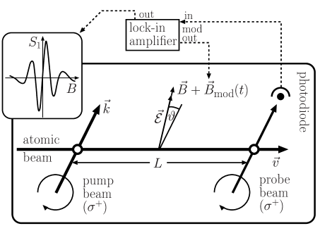
Figure 1: Experimental setup of the pump-probe experiment with circularly polarized light. The insert shows a typical experimental recording of the probe beam absorption as a function of the magnetic field. With $L=30\,\mathrm{cm}$, the period of the oscillatory structure is approximately 200 nT.

The spin polarization is measured downstream by recording the transmission of a weak circularly polarized probe laser beam. The absorption depends on the projection of the velocity averaged spin polarization on the probe laser beam. The magnetic field dependence of the transmitted intensity then leads to a damped oscillatory pattern (Ramsey fringes) symmetric around $B=0$. For practical purposes it is more convenient to work with a dispersive (antisymmetric around $B=0$) fringe pattern. Such a line shape can be generated as the derivative of the absorptive fringe pattern by applying a small amplitude modulation to the magnetic field and detecting the transmitted intensity using a lock-in amplifier locked to the modulation frequency. In additition to the well-known advantages of phase-sensitive detection, the lock-in amplifier will eliminate the $B$-independent parts of the signal which would otherwise make the pattern almost unobservable. For $\vartheta=90^{\circ}$ the resulting lineshape $S_{1}(B)$ is given by

$$S_{1}(B)\propto\int_{0}^{\infty}\sin(\gamma_{F}B\frac{L}{v})\frac{\rho(v)}{v}dv,$$

where $\rho(v)\,dv$ is the velocity distribution of the atomic density in the probe region. A typical experimental recording of such a Ramsey fringe pattern is shown as insert in figure 1. The steep central zero-crossing of this pattern is a very sensitive discriminant for the measurement of other (e.g. $\vec{\mathcal{E}}$-field induced) interactions which produce differential phase shifts of the magnetic sublevels of the ground state. Previous experiments using this technique were carried out with linearly polarized laser beams and detected the (Faraday) rotation of the probe beam polarization. This technique is closely related to the (single beam) nonlinear Faraday effect, which can be interpreted as a three-step process Weis et al. (1993a); Kanorsky et al. (1993). This resemblance, together with Ramsey’s idea of separated fields gave this method the name of Faraday-Ramsey spectroscopy (FRS) Weis et al. (1993b); Schuh et al. (1993). FRS has been used to measure the Aharonov-Casher phase shift of ${}^{85}\mathrm{Rb}$ Görlitz et al. (1995).

The key idea of the experimental technique used to measure the tensor polarizability is the following: In the interaction zone the Cs beam is exposed to parallel static electric $\vec{\mathcal{E}}$ and magnetic $\vec{B}$ fields oriented at an angle $\vartheta$ with respect to the $\vec{k}$-vector of the pump beam. When $\vec{\mathcal{E}}=0$ a feed-back loop actively stabilizes the magnetic field to the center of the dispersive central Ramsey fringe. Any additional phase shift induced by the electric field is then compensated by an automatic adjustment of the magnetic field. The corresponding compensation current $I_{\mathrm{FB}}$ in the field generating coils is the signal of interest.

For the quantitative interpretation of this compensation technique one has to know the electric field equivalent of the magnetic compensation field, which can be calculated in a straightforward way by means of the Schrödinger equation. A stretched hyperfine state $\left|F,M_{F}=F\right\rangle$ prepared in the pump region is allowed to evolve in the electric and magnetic fields. For a monochromatic beam of velocity $v$ one then obtains the wave function in the probe region, which allows to infer the $E,B$-field induced change of the probe absorption coefficient:

$$S_{1}(\Phi_{B},\Phi_{E})\propto\Phi_{B}\sin^{2}\vartheta+(2F-1)\Phi_{\mathcal{E}}\cos\vartheta\sin^{2}\vartheta,$$ (5)

where the magnetic and electric phases $\Phi_{B,\mathcal{E}}$ are given by

$$\Phi_{B}=\gamma_{F}\frac{\int B\,dl}{v}\quad\mathrm{and}\quad\Phi_{\mathcal{E}}=-\frac{3}{2F(2F-1)}\frac{\alpha_{\mathrm{2}}}{\hbar}\frac{\int\mathcal{E}^{2}\,dl}{v}.$$

The integrals are over the atomic trajectories between the pump and probe regions. As both phases have the same dependence on the atomic velocity $v$ any velocity averaging will produce a mere proportionality factor, which is irrelevant for the following discussion, and will thus be omitted. Equation 5 - derived under the assumption $\Phi_{B,\mathcal{E}}\ll 1$ - allows to define the optimal geometry and to calibrate the electrically-induced shift in terms of the magnetic compensation. As the feedback loop in the experiment adjusts the magnetic field such that $S_{1}(\Phi_{B},\Phi_{E})=0$, the signal $S$ is most sensitive to $\Phi_{\mathcal{E}}$, i.e. to the tensor polarizability, when $\vartheta$ is chosen to be the magic angle $\vartheta_{m}$, which satisfies $3\cos^{2}\vartheta_{m}-1=0$ and which maximizes the electric contribution in Equation 5. The same equation can also be used to define the magnetic equivalent of the electric phase shift, which implies

$$\frac{\alpha_{2}}{h} = \frac{F\cdot\gamma_{F}}{3\pi\cos\vartheta}\cdot\frac{\int B\,dl}{\int\mathcal{E}^{2}\,dl}$$ (6)

$$\equiv \frac{F\cdot\gamma_{F}}{3\pi\cos\vartheta}\cdot\frac{\beta}{\varepsilon}\cdot\frac{I_{\mathrm{FB}}}{U_{\mathrm{HV}}^{2}}\,.$$ (7)

Equation 7 can be understood as follows: the first factor depends on specific atomic properties and on the geometry of the experimental arrangement, while the second and third factors contain calibration constants $\beta$ and $\varepsilon$, which relate the field integrals $\int B\,dl$ and $\int\mathcal{E}^{2}\,dl$ to the feedback current $I_{\mathrm{FB}}$ and to the square of the applied high voltage $U_{\mathrm{HV}}$ respectively. Once the calibration constants are known, the tensor polarizability can be inferred from the measured dependence of $I_{\mathrm{FB}}$ on $U_{\mathrm{HV}}$.

III Experimental Setup

In the experiment, the pump and probe beams are delivered by the same extended cavity diode laser locked to the $F=4\rightarrow F^{\prime}=5$ hyperfine component of the Cs $\mathrm{D}_{2}$ transition using standard saturated absorption spectroscopy in an auxiliary vapor cell. The laser beam is transferred to the experiment proper by an optical fiber which also serves as a mode cleaner. The output intensity of the fiber is actively stabilized by a feed-back circuit controlling the input intensity with an acousto-optic modulator. The atomic beam is produced by a reflux oven Swenumson and Ewen (1981) operated at a temperature of $130^{\circ}\mathrm{C}$ and delivering a beam with a divergence of 40 mrad. Between the pump and probe zones – separated by a 30 cm long interaction zone – the atomic beam propagates in a 7 cm diameter electrically grounded tube, which contains a pair of polished copper electrodes that can be rotated around the atomic beam axis. One of the electrodes is grounded, while the other electrode is connected to a computer-controlled high voltage power supply that allows to apply electric fields up to 20 kV/cm. Two grounded diaphragms are located between the electrodes and the laser beams to ensure that the pump and probe interactions take place in an electric field-free environment. A solenoid wound on the beam tube and two pairs of rectangular coils allow to apply magnetic fields of arbitrary orientation and/or to shield unwanted field components. All coils extend over the pump and probe regions. The whole set-up is enclosed in a double cylindrical mu-metal shield (transverse / longitudinal shielding factor 14000 resp. 5800). The data acquisition (high voltage and feedback current) is controlled by a PC and the robustness of the laser frequency lock allows the experiment to be run overnight without user intervention.

IV Systematic studies and results

When $\vartheta\neq 90^{\circ}$ the motional magnetic field seen by the atoms moving through the static electric field leads to an additional magnetic phase shift, which is proportional to the electric field, i.e. to $U_{\mathrm{HV}}$. This linear Stark effect is also known as Aharonov-Casher phase shift Görlitz et al. (1995). A further noisy background may come from slowly drifting magnetic offset fields. The measurements were therefore performed in a way that allows to eliminate these backgrounds from the recorded data.

In a typical experimental run (12 hours) the data acquisition software controls the high voltage power supply by applying 5 discrete voltages $U_{i}\,(i=1,\ldots,5)$ to the electrodes, each with both polarities. We start with $U_{\mathrm{HV}}=0$ and record $I_{\mathrm{FB}}$ for two minutes. Then the software applies the voltage $U_{\mathrm{HV}}=U_{i=1}$ and records $I_{\mathrm{FB}}$ for another two minutes, after which the polarity is reversed and $I_{\mathrm{FB}}$ is recorded with $U_{\mathrm{HV}}=-U_{i=1}$ . In the next step $i$ is incremented by 1 and the cycle starts again with $U_{\mathrm{HV}}=0$. When $i=5$ is reached, the whole procedure is repeated. The integration time of 2 minutes was chosen after a detailed study of the system stability in terms of the Allan variance of $I_{\mathrm{FB}}$, which showed a minimal value for integration times between 100 and 200 seconds.

In the off-line data analysis the average value of $I_{\mathrm{FB}}$ for each cycle of a given high voltage is computed. Then the difference of time consecutive measurements with and without high voltage are calculated in order to subtract base line drifts and finally the values thus obtained for consecutive measurements with reversed polarities are averaged in order to eliminate the contribution from the motional field effect. The resulting averaged values then show a pure quadratic dependence on $U_{\mathrm{HV}}$ as illustrated in figure 2.

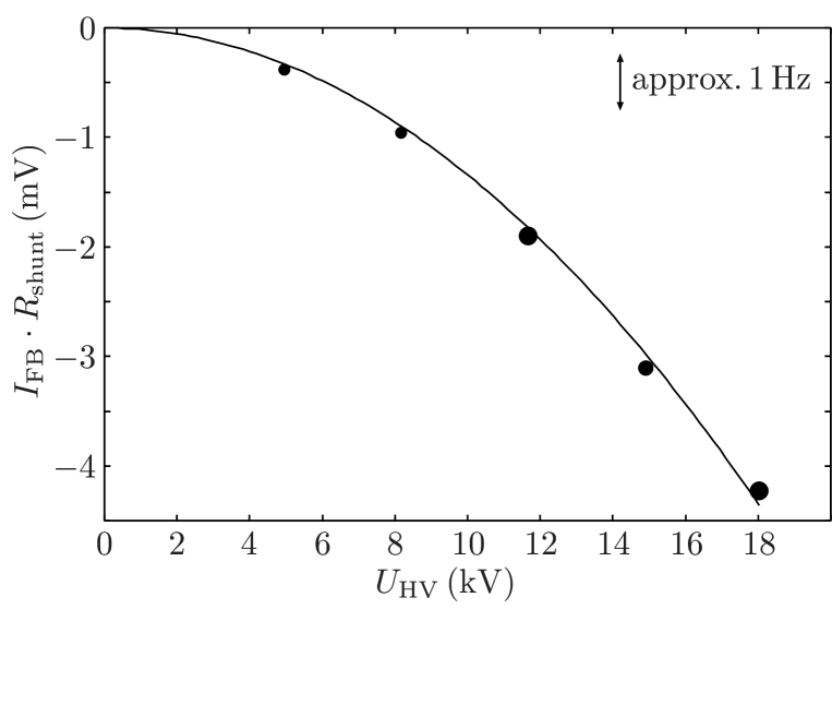
Figure 2: Quadratic Stark shift due to tensor polarizability after substraction of an offset and motional field contributions. The vertical statistical error bar of each data point corresponds to the vertical dot size. The horizontal error is negligible.

A simple quadratic fit to the data points allows, together with the calibration constants $\beta$ and $\varepsilon$, to infer $\alpha_{2}$ using equation 7 with a typical statistical error of 1% per run. The magnetic calibration constant $\beta$ was inferred from the Ramsey fringe pattern with a precision of 0.3%, while the electric calibration constant $\varepsilon$ was determined by a semi-emprical method involving both numerical calculations using an adaptive boundary element method and the Aharonov–Casher phase shift (precision of 0.3%). Details of these calibration procedures will be published elsewhere Ospelkaus et al. .

The automated measurements have allowed us to study different systematic effects. No significant dependence of the results on doubling or halving the pump laser intensity was found. This proves that the beam is fully polarized in the $\left|F=4,M_{F}=4\right>$ hyperfine state, which is a prerequisite for the validity of equation 5. There was also no detectable dependence of the results on slight misalignments of the quarter-wave plates producing the circularly polarized light, nor on variations of the oven temperature and hence the velocity distribution of the beam. Variations of the probe intensity yielded no effect on the obtained results. There is however a serious systematic uncertainty, which currently limits the absolute precision of the results. Equations 6 and 7 were derived by assuming that the magnetic and electric fields are perfectly parallel. The orientation of the electric field was realized by a mechanical rotation of the electrode structure and could be determined with an accuracy of better than 8.7 mrad. For historical reasons the rotated magnetic field was realized by adding the fields of two orthogonal pairs of coils. The contribution from the uncertainty (44 mrad) of this alignment to the final result was estimated from a systematic experimental study. The uncertainties for $\varepsilon$, $\beta$ and $\vartheta$, together with the dominating error from the relative orientation of the $\mathcal{E}$ and $B$ fields yield a (conservative) upper bound for the total systematic uncertainty of $7.5\%$.

After averaging five runs the overall statistical error is 0.7%, which leads to the preliminary result of

$$\alpha_{\mathrm{2}}(F=4)/h=-3.34(2)(25)\cdot 10^{-8}\frac{\mathrm{Hz}}{(\mathrm{V}/\mathrm{cm})^{2}},$$

where the numbers in parentheses give the statistical and systematic errors respectively. The value of $\alpha_{2}(F=4)$ inferred from previously reported Gould et al. (1969) experimental results is

$$\alpha_{\mathrm{2}}(F=4)/h=-3.66(21)(7.3)\cdot 10^{-8}\frac{\mathrm{Hz}}{(\mathrm{V}/\mathrm{cm})^{2}}\,$$

while the theoretical prediction from Angel and Sandars (1968); Sandars (1967) quoted in the article by Gould et al. is

$$\alpha_{\mathrm{2}}(F=4)/h=-4.133\cdot 10^{-8}\frac{\mathrm{Hz}}{(\mathrm{V}/\mathrm{cm})^{2}}.$$

V Conclusion and Outlook

We have demonstrated a novel technique for the measurement of tensor polarizabilities in alkali atoms. We have shown that with ${}^{133}\mathrm{Cs}$ a statistical precision below the 1% level can be achieved. The technique can easily be extended to other atoms by using suitable atomic beams and light fields. Our result is consistent with an earlier experimental result, and confirms the previously reported discrepancy with theoretical calculations at our current level of precision. In order to overcome the main current source of systematic error (parallelism of $\vec{\mathcal{E}}$ and $\vec{B}$), a new precision electrode arrangement with integrated magnetic field coils is currently under construction. With this improved set-up, a measurement of $\alpha_{\mathrm{2}}$ at the 1% level will be within reach.