A study of accuracy and precision in oligonucleotide arrays: extracting more signal at large concentrations

Abstract

Motivation: Despite the success and popularity of oligonucleotide arrays as a high-throughput technique for measuring mRNA expression levels, quantitative calibration studies have until now been limited. The main reason is that suitable data was not available. However, calibration data recently produced by Affymetrix now permits detailed studies of the intensity dependent sensitivity. Given a certain transcript concentration, it is of particular interest to know whether current analysis methods are capable of detecting differential expression ratios of 2 or higher .

Results: Using the calibration data, we demonstrate that while current techniques are capable of detecting changes in the low to mid concentration range, the situation is noticeably worse for high concentrations. In this regime, expression changes as large as 4 fold are severely biased, and changes of 2 are often undetectable. Such effects are mainly the consequence of the sequence specific binding properties of probes, and not the result of optical saturation in the fluorescence measurements. GeneChips are manufactured such that each transcript is probed by a set of sequences with a wide affinity range. We show that this property can be used to design a method capable of reducing the high intensity bias. The idea behind our methods is to transfers the weight of a measurement to a subset of probes with optimal linear response at a given concentration, which can be achieved using local embedding techniques.

Availability: Program source code will be sent electronically upon request.

Contact: felix@funes.rockefeller.edu;
soccin@rockefeller.edu; marcelo@zahir.rockefeller.edu

Introduction

High-density oligonucleotide arrays manufactured by Affymetrix are among the most sensitive and reliable microarray technology [Chee et al., 1996, Lipshutz et al., 1999] available. Based on a photolithographic oligonucleotide deposition process, labeled and amplified mRNA transcripts are probed by 22-40 (depending on chip models) short DNA sequence each 25 bases long. The probes are preferentially picked near the 3’ end of the mRNA sequence, because of the limited efficiencies of reverse transcription enzymes. In addition, the probes come in two varieties: half are perfect matches (PM) identical to templates found in databases, and the other half are single mismatches (MM), carrying a single base substitution in the middle (13th) base of the sequence. MM probes were introduced to serve as controls for non-specific hybridization, and most analysis methods postulate that the actual signal (the target’s mRNA concentration) to be proportional to the difference of match versus mismatch (PM-MM).

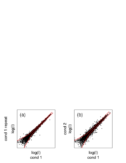
Figure 1: Typical scatterplots from GeneChip data. a) Log transformed intensities for repeated hybridization conditions (duplicates). b) different conditions. The red lines show the lines of local standard deviation (SD=2) in the log-rations.

The purpose of this work is twofold. First, we present a detailed calibration study of GeneChips. Specifically, we apply latest analysis methods (MAS 5.0 algorithm and others) to a large yeast calibration dataset, in which a number of transcripts are hybridized at known concentrations. We investigate the concentration dependence of both the accuracy and precision of differential expression scores. By accurate, we mean that the reported numerical ratios values are close to the known expression ratios, and have therefore little bias. On the other hand, a measurement is precise if it has a low noise level, also referred to as small variance. Our results show that the ability of conventional analysis techniques to detect small changes strongly deteriorates toward high transcript concentrations. While the variance is smallest for high concentrations, it appears that the question of the bias in this regime has been neglected. In fact, the bias is strong enough that real changes of 2 (even 4) can often not be detected. This sounds at first counter-intuitive, which we believe is rooted in the following widespread interpretation of hybridization data. Namely, when examining the data from two replicated conditions (Figure 1a) most would focus on the low intensity region, and observe how noisy this regime appears to be in comparison to the high-intensity tail. However, this view is misleading, as it does not consider the question of the bias. Turning to a comparison of two different conditions (Figure 1b), we notice that the noise envelope is essentially unchanged, and that real changes appear as points lying distinctively outside the noise cloud. Looking at multiple such comparisons, we would then conclude that the high intensity data is almost always very tightly scattered about the diagonal, and that there are rarely genes in that region that show fold changes greater than, say, 1.5 or 2. The interpretation that no differential regulation occurs in highly expressed transcripts seems unlikely. In fact, we show evidence that real changes are often compressed for large concentrations. This saturation effect can actually be observed in Affymetrix’s own data although the issue is not commented there (a qualitative report has been given in [Chudin et al., 2001]). The physical origin for the compression effect invokes non-linear probe affinities and chemical saturation. This is a separate issue from optical saturation (cf. Results). Chemical saturation occurs below the detector threshold and is attributed to the fact that some probes will exhaust their binding capacities at relatively low concentrations, simply because their binding affinities are high. Binding affinities are in fact very sensitive to the sequence composition, resulting in measured brightnesses that usually vary by several decades within a given probeset [Naef et al., 2002].

Our second goal is to present an analysis method that reduces the bias at high concentrations. Our approach uses all PM and MM probes equally, in contrast to the standard view in which the PMs are thought to carry the signal, while the MMs serve as non-specific controls. In fact, it has become clear that the MM probes also track the signal, usually with lower (although often with higher) affinities than the PM’s [Naef et al., 2002]. In that sense, the MM’s should be viewed as a set of on average lower affinity probes. It is then reasonable to expect that some MM probes will more accurate at high intensities, since they will be less affected by saturation than the the PM’s (cf. Figure  3).

Methods

The existing methods for the analysis of the raw data fall into two main classes. The first methods are similar to Affymetrix’s Microarray Suite software, providing absolute intensities on a chip by chip basis, or differential expression ratios from two experiments [Affymetrix, 2001, Naef et al., 2001, Naef et al., 2002]. The second class are called “model-based” approaches [Li & Wong, 2001], and attempt to fit the probe affinities from a large number of experiments.

The method described below belongs to the second class and is specifically designed for improved accuracy in the compressive high-intensity regime. It is based on ideas borrowed from the theory of locally linear embeddings [Roweis & Saul, 2000].

Notation

We construct the following matrix

$$A^{j}_{i} = \left\{\begin{array}[]{cc}{\it PM}_{i}^{j}&1\leq j\leq N_{p}\\ {\it MM}_{i}^{(j-N_{p})}&N_{p}<j\leq 2N_{p}\end{array}\right.$$

or in expanded notation

$$A^{j}_{i} = \left[\begin{array}[]{cccccc}{\it PM}_{1}^{1}&\cdots&{\it PM}_{1}^{N_{p}}&{\it MM}_{1}^{1}&\cdots&{\it MM}_{1}^{N_{p}}\\ \vdots&{\it PM}_{i}^{j}&\vdots&\vdots&{\it MM}_{i}^{j}&\vdots\\ {\it PM}_{N_{e}}^{1}&\cdots&{\it PM}_{N_{p}}^{N_{e}}&{\it MM}_{N_{e}}^{1}&\cdots&{\it MM}_{N_{p}}^{N_{e}}\\ \end{array}\right]$$

which contains the raw, background subtracted and normalized data. By background, we mean fluorescence background, which we identify by fitting a Gaussian distribution to the subset of all $(PM,MM)$ pairs satisfying the criterion that $|PM-MM|<\epsilon$, with $\epsilon=50$. This provides us with the mean and SD in the background fluorescence. . For a fair comparison of compression effects in various methods, we used the global normalization factors from the MAS 5.0 software in all cases, however, the technique remains applicable with other normalization schemes.

$N_{p}$ is the number of probe pairs and $N_{e}$ is the number of experiments. We introduce a set of weights $w_{i}$ such that

$$\sum_{i=1}^{N_{e}}\,w_{i}=1$$

and define the column means (or center of mass)

$$m^{j}=\sum_{i=1}^{N_{e}}\,w_{i}\,{\log(A^{j}_{i})}$$

Note, we are computing the mean of the logs of the components of $A_{i}^{j}$.

Local principal component analysis

Local embeddings are adequate in situations where compression is important because non-linearities (resulting from chemical saturation) affect the one-dimensional manifold $\{{\it PM}^{j}(c),\,{\it MM}^{j}(c)\}$ (the concentration $c$ is the one-dimensional ’curve’ parameter) by giving it a non-zero local curvature. The results section, in particular Figure 3 contains ample evidence that these non-linearities are significant (cf. also Figure 2 in [Chudin et al., 2001]). Our method is a multidimensional generalization of the schematic depicted in Figure 2, which shows the typical situation of two probes in which one of the probes (PM2) saturates at concentrations lower than the other. If both probes were perfectly linear, the curve would be a straight line with slope 1. In the multidimensional case, the directions of largest variation (analogous to D1 or D2 in Figure 2) are computed from the principal components of the matrix

$$\sqrt{{w_{i}}}\,\left({\log(A^{j}_{i})}-m^{j}\right)=\sum_{k=1}^{N_{p}}U_{ik}\,D_{k}\,V^{j}_{k}$$

which can easily be done via singular value decomposition (SVD). In order to reconstruct the concentrations, one needs first to consider the unspecified sign of the vector $V^{j}_{1}$ (when returned by the SVD routine), which has to be chosen such that the total amount of signal comes out positive. This is easily achieved by adjusting the sign of $V^{j}_{1}$ such that $\sum_{i,j}\,{\log(A^{j}_{i})}\,V^{j}_{1}>0$ . The logarithm of the concentration $s_{i}$, is then computed by projecting the original matrix onto the first principal component $V^{j}_{1}$, corrected by a factor $v_{max}$. This factor accounts for the fact that the vector $V^{j}_{1}$ is $L_{2}$-normalized ($\sum_{j}\,(V^{j}_{1})^{2}=1$) by definition in the SVD. The signal then reads:

$$s_{i}={v_{\it max}}\,\sum_{j=1}^{N_{p}}{\log(A^{j}_{i})}\,V^{j}_{1}$$

where ${v_{\it max}}=\max_{j}\left|V^{j}_{1}\right|$. In addition, the above procedure automatically yields a signal-to-noise ($S/N$) measure for the entire probeset

$$\frac{S}{N}=\frac{D_{1}}{\sqrt{\sum^{N_{p}}_{j=2}\,D^{2}_{j}}},$$

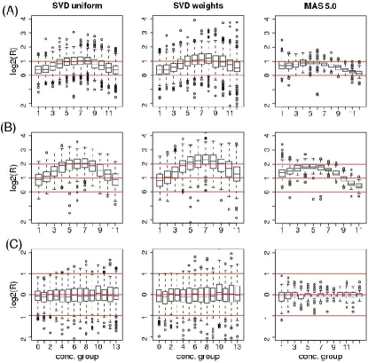
Figure 4: Rows are as in Figure 3, columns show the new method with uniform (first column), Cauchy weights introduced in the text (second), and the reference MAS5.0 (third).

where $\{D_{k}\}$ are the singular values. Large $S/N$ values imply that the probeset measurements in the $N_{e}$ experiments had a well-defined direction of variation, and can for instance be used as a filter for identifying genes that exhibit significant changes across the experiments tested. In the results shown in Figure 4, we used the following weights

$$w_{i}=\frac{1}{W}\left\{\begin{array}[]{cl}1,&\hat{s}_{i}>\Gamma,\\ 1/\!\left({1+b\,(i-{i_{s}})^{2}}\right),&\hat{s}_{i}\leq\Gamma\end{array}\right.$$

where $W=\sum_{i}\,w_{i}$, $\hat{s}_{i}$ is the signal obtained with uniform weights, ${i_{s}}=20$ (out of 28 experiments), $b=2$, and $\Gamma=\hat{S}_{{i_{s}}+1}$ with $\hat{S}_{i}$ being the ascendantly sorted $\{\hat{s}_{i}\}$. In other words, lower concentration points are suppressed according to their rank (computed with uniform weights) using a slowly decaying Cauchy weight function. There are of course other weight functions that could serve the same purpose.

Note that the fitting procedure used in the Li-Wong [Li & Wong, 2001] method is identical to an SVD decomposition, however, with different input data than was use here. The three main difference between our method and the Li-Wong technique are: (i) in the analysis here, we used log transformed PM  and MM  intensities, rather than the bare PM-MM values; (ii) we introduced optional weights, which can account for non-linearities of the probe response in the high concentration regime; (iii) we subtract the column mean before we compute the principal components, which is crucial for capturing the local directions of variation. Indeed, as can be seen in Figure 2, the principal component would be dominated by the mean itself without subtraction.

Results

Data sets

The yeast Latin square (LS) experiment is a calibration data set produced by Affymetrix, that uses a non-commercial yeast chip. 14 groups of 8 different genes, all with different probe sets, are spiked onto 14 chips at concentrations, in pM, corresponding to all cyclic permutations of the sequence (0, 0.25, 0.5, 1, 2, $\ldots$, 1024). Hence, each group is probed at 13 different finite concentrations, logarithmically spaced over a range of magnitudes from 1 to 4096 (in Figures 3 and 4, we refer to these concentrations as ($1=0.25\,\rm pM$, $2=0.5\,\rm pM$ $\ldots$ $13=1024\,\rm pM$), and each group is completely absent in one array. Besides the spiked-in target cRNA’s, a human RNA background was added to mimic cross-hybridization effects that would occur in a real experiment. In addition, each experiment was hybridized twice leading to 2 groups of 14 arrays called R1 and R2.

The reason why this dataset is attractive as compared to the similar human and e. coli datat available at www.netaffx.com are several. First, the e. coli data exhibits severe optical saturation, which interfers with the chemical saturation issue we are trying to address here. The yeast dataset, on the other hand, has virtually no optically saturated cells, as can be inferred the SD in the pixel intensities reported in the raw data (.CEL) files. In total, fewer than $0.1\%$ of the probes have $SD=0$ ($SD=0$ characterizes optical saturated cells). Further, optical saturation is no longer an issue in GeneChips with the current scanner settings. More important, the present dataset permits far better statistics, as the number of spiked-in genes is 112 as compared to 14 for the human chip. In the latter dataset, there is only one transcript per concentration group as compared to 8 in the yeast case. In fact, we verified that the compression effects discussed below are virtually identical in the human case (not shown).

Summary of two-array methods

The figures in the results section show the log-ratios as function of concentration in the form of boxplots. In these plots, the central rectangle indicates the median, 1st and 3rd quartiles ($Q1$ and $Q3$). The “whiskers” extend on either side up to the last point that is not considered an outlier. Outliers are explicitly drawn and are defined as laying outside the interval $[Q1-1.5*IQ,\,Q3+1.5*IQ]$, where $IQ=Q3-Q1$ is the interquartile distance. For each method, we show three plots, the top two measure the false negative rate for ratios of 2 and 4 fold respectively, and the last one shows the false positive rate. For the top two plots, all combinations (within R1 and R2 separately) of arrays leading to ratios of 2 and 4 were considered, and plotted as function of their baseline intensity (the lesser of the two concentrations). For the third, each gene was compared between the groups R1 and R2, at identical concentrations. Of the $8*14=112$ transcripts, 8 were left out of the analysis because they did not lead to a signal that was tracking the concentrations at all (presumably due to bad probes or transcript quality).

In Figure 3, we summarize the results obtained by the Microarray Analysis Suite 5.0 (MAS 5.0) software and the “2 chips” method discussed in [Naef et al., 2002]. The later method computes for each gene probed in two arrays a ratio score $R$ such that

$$\log(R)=\sum_{j}^{robust}\log(R^{j})$$

is a robust geometric mean (a least trimmed squares estimator) of the probe ratios $R^{j}$. Figure 3 shows the cases where

$$R^{j}=\frac{{\it PM}^{j}_{1}-{\it MM}_{1}^{j}}{{\it PM}^{j}_{2}-{\it MM}^{j}_{2}}$$

and

$$R^{j}=\frac{{\it MM}_{1}^{j}}{{\it MM}^{j}_{2}}$$

In both cases, only probes with numerator and denominator above background are retained. The first case (${\it PM}-{\it MM}$) is in essence similar to the MAS 5.0 program, differences are in the choice of the Tuckey bi-weight mean as the robust estimator, and in the treatment of negative differences. For our purpose here, we like to think of the Affymetrix method as two-array, ${\it PM}-{\it MM}$ based method. In all the results presented below, the arrays were scaled according to the MAS 5.0 default settings.

The main features of Figure 3 are: there is an optimal range of baseline concentrations ($\approx 1-16$ pM) in which the ratio values from both ${\it PM}-{\it MM}$ methods (the two first columns) are fairly accurate, for both ratios of 2 and 4. For both lower and higher concentrations, there is a noticeable compression effect, which is most dramatic at the high end. At the highest baseline concentration (512 pM for the ratios of 2 and 256 pM for ratios of 4), changes of 2 are basically not detected and real changes of 4 are compressed on average to values around 1.25. The analysis of the false positive rate (last row) shows that both methods yield very tight reproducibility: the log2 ratio distributions are well centered around 0 and the interquartile distances are roughly intensity independent and smaller than $~{}0.2$, meaning that 50% of the measurements fall in the ratio interval $[0.93,1.07]$. To be fair, we should point out that as a (${\it PM}-{\it MM}$) method, the MAS 5.0 algorithm is on average a bit cleaner, having slightly fewer outliers. However, we like to emphasize that the qualitative behavior in the two (${\it PM}-{\it MM}$) methods is unchanged, especially as far as the high-intensity compression is concerned. Further, similar behavior is also found using the (${\it PM}-{\it MM}$) Li-Wong method (data not shown). The above observations are consistent with what was reported in [Chudin et al., 2001], confirming that these effects are independent of the chip series.

The third column in Figure 3 illustrates our contention that the MM are in essence a set of lower affinity probes. We notice that using only the MM measurements in the two-array method changes the picture qualitatively. Whereas the low concentration regime is far worse than in the (${\it PM}-{\it MM}$) methods, the behavior toward the high end has changed and the drop off occurs now at higher concentrations: approximately 256 pM for the ratios of 2 and 128 pM for ratios of 4. On the other hand, even in the optimal range, the magnitude of the medians are always a bit lower than the real ratios, and the false positive rate also suffers. To summarize, this result suggests that if one is interested in accuracy at high concentrations, then the MM-only methods offers the best two-array alternative. We have tried other variations: PM only, or the double size set consisting in the merged PM and MM’s, both being worse at high concentrations than the MM only method.

Multi-array methods

The data analyzed using our new method is shown in Figure 4. It is clear that both are capable of reducing the high intensity compression, as compared to existing methods. The second column explicitly shows the higher accuracy of the local method. It should be noted, however, that the precision is significantly lower than with MAS 5.0, which is the trade-off to pay for higher signal detection. As compared to the “two chip” MM method, which was previously the least compressive in this regime, the medians are systematically more accurate. Also, the method does not perform well at low-concentrations which is expected since it was not designed for that range.

Significance scores

Although ratio score may suffer severe compression, there remains the possibility that they would be attributed a significant increase or decrease call. Figure 5 displays the relation between the MAS 5.0 log-ratios and their associated p-values. MAS 5.0 change ‘p-values’ $p_{M}$ are symmetric about 0.5 and designed such that the ratio score is called increased when $p_{M}<\gamma_{1}$ and decreased (D) when $p_{M}>1-\gamma_{1}$, with a default $\gamma_{1}=0.0025$. This definition is not well suited for plotting purposes, we therefore work with $p_{\it MAS}=p_{M}$ when $p_{M}<0.5$, and $p_{\it MAS}=1-p_{M}$ otherwise. This way, both I and D genes have $p_{\it MAS}<\gamma_{1}$, the direction being given by the sign of the log-ratio. The results show that there remarkably few false positive calls: only 4 out of 624 for concentrations $c\leq 8\,\rm pM$, and 6 of 728 when $c\geq 16\,\rm pM$. Fold changes of 4 are also well detected despite the compression at high intensities: there are 21 false negatives (and 3 false positives having ratios with the wrong sign) out of 1248 for $c\leq 8\,\rm pM$, and 84 of 1040 false negatives for $c\geq 16\,\rm pM$. The situation deteriorates for fold changes of 2, with 124 false negatives (and 3 false positives) out of 1248 for $c\leq 8\,\rm pM$, and 425 of 1248 false negatives for $c\geq 16\,\rm pM$.

Discussion

We have shown that high-concentration bias is a serious issue in GeneChips, which is probably related to chemical saturation in the adsorption process of the target to the probes. Exploiting the broad range of affinities of different probes (PM and MM included) offers an approach toward improvements. However, the gain in accuracy comes with an expected decrease in precision, since effectively, the weight of a measurement is transferred to a smaller set of probes. Hence, the reduction in noise levels resulting from averaging over probes is diminished.

Our method should serve as a useful complement to those who use microarrays primarily as a gene discovery tool, and are interested in maximal signal detection. In fact, we often hear that severe constraints like pharmaceutical treatments or gene knockouts appear to have no detectable transcriptional effects. While there is the possibility that transcription regulatory networks can compensate for such changes, or that some effects would be mostly post-transcriptional, real transcriptional changes may also be masked by compressive effects like those discussed above.

Conclusion

We have summarized the performance of existing methods for analyzing Affymetrix GeneChip data, using the yeast calibration dataset from Affymetrix. The results show unambiguously the compressive tendency of GeneChip measurements in the high-intensity range, namely that fold changes as large as 4 in expression levels can be reduced to fold changes barely larger than 1 (Figure 3). Interestingly, we showed that among the standard techniques, the one using only the MM signals offers the highest accuracy at high concentrations. Additionally, we have how it is possible to achieve higher accuracy at high concentrations by exploiting the probeset’s wide affinity range. One should realize, however, that saturation problems of the sort encountered present a hard challenge in signal processing, and it is therefore expected that higher accuracy is obtained at the expense of reduced precision.

Our observations raise the following design issue for oligonucleotide arrays. Since it will likely be difficult to manufacture oligonucleotide probes with linear responses over 4 or more decades in concentration, an option would be to optimize the design of probesets such that each of its probe would be optimally linear in smaller ranges (say 2 decades at most) centered around graded concentrations. In this way, the weights of a measurement could be transferred to an appropriate subset of probes known to be optimal in a given range. Hence, one would use a different set of probes for high or low concentration values to increase the overall dynamic range of a probeset.

Figures

Figure 2: Typical compressive situation: a 2 dimensional cartoon. The open dots represent fictitious measurement of two probes (PM1, PM2) at increasing concentrations (from left to right). Probe PM2 saturates earlier than PM1. $M1=(m^{1},\,m^{2})$ represents the mean with uniform weights $\{w_{i}\}$ and M2 a mean obtained with weights that are larger for high concentrations. D1 and D2 show the corresponding principal components (direction of largest variance). It is clear that projecting the points onto D1 has the effect of a compression due to the curvature. On the other hand, this compression is largely reduced at high-intensities by projecting onto D2.

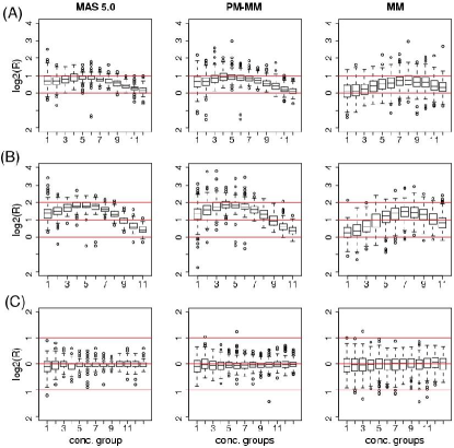
Figure 3: Comparison of ’two array’ methods: MAS 5.0 (first column), ${\it PM}-{\it MM}$ (second) and MMonly (third) of [Naef et al., 2002]. Boxplots show the log base 2 ratio distributions for each baseline concentration group (cf. text). Row A: Fold change of 2, B: Fold change 4, C: Negative controls (false positives). The central rectangle indicates the median, 1st and 3rd quartiles ($Q1$ and $Q3$). The “whiskers” extend on either side up to the last point which is not considered to be an outlier. Outliers are explicitly drawn and are defined as laying outside the interval $[Q1-1.5*IQ,\,Q3+1.5*IQ]$, where $IQ=Q3-Q1$ is the interquartile distance. Notice the two first rows are qualitatively similar, with the MAS 5.0 being marginally cleaner. Both methods show a strong high concentration compression, but have excellent reproducibility (cf. text). The third column illustrates that MM probes contain valuable signal, often leading to more accurate ratios at high concentrations.

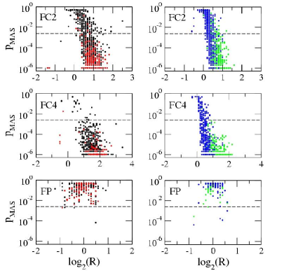
Figure 5: P-values vs. log-ratios in for MAS 5.0. The plotted $p_{MAS}$ is the transformed MAS 5.0 p-value (cf. text). The dotted line indicates the default $\gamma_{1}=0.0025$, below which MAS 5.0 scores are considered increased (I) or decreased (D) (for the transformed p-value). Colors are used to group baseline intensities of 0.25–1 pM (black), 2–8 pM (red), 16–64 pM (green), 128–1024 (blue).

References

- Affymetrix, 2001 Affymetrix (2001) Affymetrix Microarray Suite 5.0 User Guide. Affymetrix, Inc., Santa Clara, CA.
- Chee et al., 1996 Chee, M., Yang, R., Hubbell, E., Berno, A., Huang, X. C., Stern, D., Winkler, J., Lockhart, D. J., Morris, M. S. & Fodor, S. P. (1996) Accessing genetic information with high-density DNA arrays. Science, 274 (5287), 610–614.
- Chudin et al., 2001 Chudin, E., Walker, R., Kosaka, A., Wu, S. X., Rabert, D., Chang, T. K. & Kreder, D. E. (2001) Assessment of the relationship between signal intensities and transcript concentration for affymetrix genechip(r) arrays. Genome Biol., 3 (1), Research0005.
- Li & Wong, 2001 Li, C. & Wong, W. H. (2001) Model-based analysis of oligonucleotide arrays: expression index computation and outlier detection. Proc. Natl. Acad. Sci. U. S. A., 98 (1), 31–36.
- Lipshutz et al., 1999 Lipshutz, R. J., Fodor, S. P., Gingeras, T. R. & Lockhart, D. J. (1999) High density synthetic oligonucleotide arrays. Nat. Genet., 21 (1 Suppl), 20–24.
- Naef et al., 2002 Naef, F., Hacker, C. R., Patil, N. & Magnasco, M. (2002) Empirical characterization of the expression ratio noise structure in high-density oligonucleotide arrays. Genome Biol., 3 (4), research0018.1–0018.11.
- Naef et al., 2001 Naef, F., Lim, D. A., Patil, N. & Magnasco, M. (2001) From features to expression: high-density oligonucleotide array analysis revisited. In Proceedings of the DIMACS Workshop on Analysis of Gene Expression Data The American Mathematical Society.
- Naef et al., 2002 Naef, F., Lim, D. A., Patil, N. & Magnasco, M. (2002) DNA hybridization to mismatched templates: a chip study. Phys. Rev. E, 65, 040902.
- Roweis & Saul, 2000 Roweis, S. T. & Saul, L. K. (2000) Nonlinear dimensionality reduction by locally linear embedding. Science, 290 (5500), 2323–2326.