Multiple scattering of light by atoms with internal degeneracy

Abstract

An analytical microscopic theory for the resonant multiple scattering of light by cold atoms with arbitrary internal degeneracy is presented. It permits to calculate the average amplitude and the average intensity for one-photon states of the full transverse electromagnetic field in a dilute medium of unpolarized atoms. Special emphasis is laid upon an analysis in terms of irreducible representations of the rotation group. It allows to sum explicitly the ladder and maximally crossed diagrams, giving the average intensity in the Boltzmann approximation and the interference corrections responsible for weak localization and coherent backscattering. The exact decomposition into field modes shows that the atomic internal degeneracy contributes to the depolarization of the average intensity and suppresses the interference corrections. Static as well as dynamic quantities like the transport velocity, diffusion constants and relaxation times for all field modes and all atomic transitions are derived.

1 Introduction

Wave propagation in disordered media has been an active field of research for more than a century. The first descriptions of electronic conduction in weakly disordered metals by Drude [1] and of light propagation in interstellar clouds by Schuster [2] were based on Boltzmann-type transport equations. Despite their successful predictions (e.g. Ohm’s law), these theories overlooked the subtle role of interference. P. Anderson first showed that sufficiently strong disorder can induce a metal-insulator transition for quantum-mechanical wave functions on a random lattice, a phenomenon baptized Anderson localization [3]. Furthermore, it was realized that interference influences transport even far from the localization transition and that also other waves are concerned. For example, the constructive interference of counter-propagating light amplitudes in the backward direction, as first pointed out by Watson [4], survives an average over disorder, giving rise to the coherent backscattering (CBS) peak [5, 6, 7]. In the past 20 years, the field of mesoscopic physics has developed, with beautiful experimental and theoretical results pertaining to the weak localization regime [8, 9, 10].

Atoms, as natural realizations of highly resonant identical point scatterers, have been proposed as an ideal sample for multiple light scattering and even localization [11, 12]. However, as first discovered in experiments on CBS by rubidium atoms [13, 14] and recently confirmed on strontium atoms [15], the quantum internal structure of atomic scatterers has a strong impact on light transport properties. The Zeeman degeneracy of the probed dipole transition reduces the interference contrast of coherent backscattering [16] dramatically. The single and double scattering contribution to the CBS peak for atoms with arbitrary internal degeneracy have been calculated in [17].

In the present contribution, we develop an analytical theory of multiple resonant one-photon elastic scattering in an infinite medium consisting of a dilute gas of cold atoms at fixed classical positions, but with arbitrary internal degeneracy. Our results are a first step towards a microscopic generalization of the existing theories for the scattering of transverse vector waves by Rayleigh point scatterers [18, 19] on the one hand and of scalar waves by anisotropic scatterers [20, 21] on the other. The paper is organized as follows. In section 2, we define the Hamiltonian for the coupled system light and atoms. In section 3, we calculate the average propagator of a one-photon Fock state inside the scattering medium with the aid of the Dyson equation and the photon self-energy. In section 4, we define the average intensity for the full vector field in terms of photo-detection probability. The corresponding Bethe-Salpeter equation is then solved by evaluating the so-called irreducible vertex in the Boltzmann approximation. Technically, this is achieved by a systematic analysis in terms of irreducible tensor operators. In section 5, we sum the so-called ladder series in the static limit by applying the same method of irreducible tensors to the intensity propagator of transverse field modes. The interference correction described by the maximally crossed diagrams is then easily obtained by applying substitution rules. In section 6, we generalize our results to the dynamic case and derive analytical expressions for transport velocities, diffusion constants, extinction lengths and relaxation times for the different field modes and all atomic transitions. We conclude by possible extensions of the work.

2 Description of the system

2.1 Hamiltonian

In order to analyze the role of the atomic quantum internal structure, we must treat the atomic internal degrees of freedom quantum mechanically. For reasons of symmetry, the light field is treated quantum mechanically as well. Using natural units such that $\hbar=c=1$, the global system “matter + light” is then described by the Hamiltonian $H=H_{0}+V$ where

$$H_{0}=H_{\mathrm{em}}+H_{\mathrm{at}}=\sum_{{\bf k},\boldsymbol{\varepsilon}\perp\bi k}\omega_{\bi k}\>a_{\bi k\boldsymbol{\varepsilon}}^{\dagger}a_{\bi k\boldsymbol{\varepsilon}}+\sum_{\alpha=1}^{N}H_{\mathrm{at}}(\alpha).$$ (1)

$H_{\mathrm{em}}$ is the Hamiltonian of the free electromagnetic field. The annihilation and creation operators for the field modes (wave vector $\bi k$, transverse polarization $\boldsymbol{\varepsilon}$, free dispersion relation $\omega_{\bi k}=k$) obey the usual bosonic commutation relation $[a_{{\bi k}\boldsymbol{\varepsilon}},a_{{\bi k^{\prime}}\boldsymbol{\varepsilon}^{\prime}}^{\dagger}]=\delta_{\boldsymbol{\varepsilon},\boldsymbol{\varepsilon}^{\prime}}\delta_{\bi k,\bi k^{\prime}}$. For brevity, a one-photon Fock state will be noted $|\bi k\boldsymbol{\varepsilon}\rangle\equiv a_{\bi k\boldsymbol{\varepsilon}}^{\dagger}|0\rangle$ where the transversality $\boldsymbol{\varepsilon}\cdot\bi k=0$ is understood. $H_{\mathrm{at}}$ is the sum of the individual internal atomic Hamiltonians

$$H_{\mathrm{at}}(\alpha)=\omega_{0}\sum_{m_{\mathrm{e}}=-J_{\mathrm{e}}}^{J_{\mathrm{e}}}|J_{\mathrm{e}}m_{\mathrm{e}}(\alpha)\rangle\langle J_{\mathrm{e}}m_{\mathrm{e}}(\alpha)|.$$ (2)

Each atom $\alpha=1,\dots,N$ is described as a degenerate closed two-level system with an energy separation $\omega_{0}$ between the ground-state with total angular momentum $J$ and the excited-state with total angular momentum $J_{\mathrm{e}}$ (figure 1). These levels are resonantly coupled by the dipole interaction

$$V=\sum_{\alpha=1}^{N}V_{\alpha}=-\sum_{\alpha=1}^{N}\bi D_{\alpha}\cdot\bi E(\bi r_{\alpha}).$$ (3)

The individual atomic dipole operator $\bi D_{\alpha}$ acts on the Hilbert space $\mathcal{H}_{\mathrm{g}}\oplus\mathcal{H}_{\mathrm{e}}$ of the internal atomic states of atom $\alpha$. Dropping subscript $\alpha$, we define the reduced dipole operator $\bi d=\bi D/d$ where $d=\langle J_{\mathrm{e}}||\bi D||J\rangle/\sqrt{2J_{\mathrm{e}}+1}$. The matrix elements of its spherical components $d_{q}\equiv\bi e_{q}\cdot\bi d$, $q=-1,0,+1$ are the Clebsch-Gordan coefficients $\langle J_{\mathrm{e}}m_{\mathrm{e}}|d_{q}|Jm\rangle=\langle J_{\mathrm{e}}m_{\mathrm{e}}|J1mq\rangle$ according to the Wigner-Eckhart theorem [22]. In the dipole interaction, the electric field operator

$$\bi E(\bi r)=\rmi\sum_{\bi k,\boldsymbol{\varepsilon}\perp\bi k}\mathcal{E}_{\omega}\left(\boldsymbol{\varepsilon}_{\bi k}a_{\bi k\boldsymbol{\varepsilon}}\rme^{\rmi\bi{k}\cdot\bi{r}}-\boldsymbol{\bar{\varepsilon}}_{\bi k}a_{\bi k\boldsymbol{\varepsilon}}^{\dagger}\rme^{-\rmi\bi{k}\cdot\bi{r}}\right)$$ (4)

is evaluated at the center of mass $\bi r_{\alpha}$ of each scattering atom. The field oscillator strength $\mathcal{E}_{\omega}=(\omega/2\epsilon_{0}L^{3})^{1/2}$ is given in terms of a quantization volume $L^{3}$ that will disappear from physically relevant expressions in the limit of an infinite medium by virtue of the rule $L^{-3}\sum_{\bi k}(\dots)\mapsto(2\pi)^{-3}\int{\mathrm{d}}^{3}k(\dots)$.

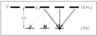
Figure 1: Resonant degenerate dipole transition, here for $J=1$, $J_{\mathrm{e}}=2$. The atomic resonance frequency is noted $\omega_{0}$, the detuning of the light probe $\delta=\omega-\omega_{0}$, and the natural width of the excited atomic state $\Gamma$. The internal magnetic quantum numbers $m$ are coupled to the polarization of scattered photons (full and dotted lines).

2.2 Length scales hierarchy

The detailed description of wave propagation in a large sample of scatterers at quenched random positions is such a formidable task that one rather resorts to a statistical description, catching the generic features through configuration averaged quantities (average amplitude, average intensity, etc) [23, 24, 25]. In the following, we will consider the limit of a disordered infinite medium where resonant point scatterers are distributed with constant spatial density $n$. The absence of boundaries greatly simplifies the theory since translational symmetry is restored on average. The importance of interference depends essentially on the hierarchy between the physically relevant length scales in the system, here the wave length $\lambda$ and the mean inter-particle distance $n^{-1/3}$. We will concentrate on the low density regime where $\lambda\ll n^{-1/3}$. This inequality, alternatively rewritten as $n\lambda^{3}\ll 1$, justifies a semi-classical description of propagation along rays between consecutive scatterers that define scattering paths and their associated amplitudes. It also implies that scattering paths involving different scatterers are uncorrelated: since their phase difference greatly exceeds $2\pi$, the associated interference term can be expected to average to zero. Also, recurrent scattering sequences (visiting a given scatterer more than once) can be neglected: this is the independent scattering approximation (ISA) [23]. In this dilute regime, the elastic mean free path (mean distance traveled between two successive scattering events) is given by $\ell=1/n\sigma$ where $\sigma$ is the total cross-section for elastic scattering. Since we treat resonant point scatterers where $\sigma\sim\lambda^{2}$, the low density condition implies $\lambda\ll\ell$: wave scattering is described in the far field. On the same ground, the equivalent relation $\sqrt{\sigma}\ll\ell$ shows that recurrent scattering is indeed negligible. And finally, the low density condition implies $k\ell\gg 1$ where $k=2\pi/\lambda$, which defines the weak localization regime.

3 Average light propagation

The simplest quantity of interest for wave propagation in random media is the average amplitude, so we first compute the configuration-averaged propagator $\left\langle G(\omega)\right\rangle$.

3.1 The one-atom scattering operator

In the weak localization regime, a scattered wave has reached its asymptotic limit when undergoing a subsequent collision. Hence a central quantity in the theory is the one-atom transition operator $T_{\alpha}(z)$, given by the Born series $T_{\alpha}(z)=V_{\alpha}+V_{\alpha}G_{0}(z)V_{\alpha}+\dots$ in powers of the interaction $V_{\alpha}$ and the free resolvent operator $G_{0}(z)=(z-H_{0})^{-1}$ [26]. The scattering amplitude associated to the elastic scattering process $|i\rangle=|\bi k\boldsymbol{\varepsilon};Jm\rangle\to|f\rangle=|\bi k^{\prime}\boldsymbol{\varepsilon}^{\prime};Jm^{\prime}\rangle$ is proportional to

$$\langle f|T_{\alpha}(\omega+\rmi 0)|i\rangle=\langle Jm^{\prime}|\boldsymbol{\bar{\varepsilon}}^{\prime}\cdot\bi t(\omega)\cdot\boldsymbol{\varepsilon}|Jm\rangle\,\rme^{\rmi(\bi k-\bi k^{\prime})\cdot\bi r_{\alpha}}$$ (5)

where the notation $\omega+\rmi 0$ indicates that retarded propagators are used in the Born series and that the matrix elements are taken on-shell ($\omega=\omega_{\mathrm{\bi k}}=\omega_{\mathrm{\bi k^{\prime}}}$). Note that the incident and scattered wave vector appear only in the exponential on the right hand side: in the dipole approximation, the atom indeed behaves as a point scatterer, and the external and internal degrees of freedom are factorized. The frequency dependence of the internal transition operator $\bi t(\omega)$ is

$$t(\omega)=\frac{3}{2\pi\rho_{0}(\omega)}\frac{\Gamma/2}{\delta+\rmi\Gamma/2}$$ (6)

where $\Gamma=d^{2}\omega_{0}^{3}/3\pi\epsilon_{0}$ is the natural width of the excited atomic state, $\delta=\omega-\omega_{0}$ is the detuning of the probe light from the atomic resonance and $\rho_{0}(\omega)=L^{3}\omega^{2}/2\pi^{2}$ is the free photon spectral density. This form of a resonant scalar t-matrix is well known in the context of classical point scatterers [27]. But as the atomic scatterer has an internal structure, particular attention must be paid to the tensor character of the scattering operator. For a given atomic transition $m\mapsto m^{\prime}$, the Cartesian elements of the t-matrix are

$$t_{ij}(m,m^{\prime},\omega)=t(\omega)\langle Jm^{\prime}|d_{i}d_{j}|Jm\rangle.$$ (7)

This $3\times 3$ t-matrix can be decomposed into its irreducible components with respect to rotations, its scalar part (or trace), its antisymmetric part and symmetric traceless part:

$$t_{ij}=\underbrace{\frac{1}{3}\delta_{ij}t_{kk}}_{\displaystyle t_{ij}^{(0)}}+\underbrace{\frac{1}{2}(t_{ij}-t_{ji})}_{\displaystyle t_{ij}^{(1)}}+\underbrace{\frac{1}{2}(t_{ij}+t_{ji})-\frac{1}{3}\delta_{ij}t_{kk}}_{\displaystyle t_{ij}^{(2)}}$$ (8)

In the case of a point dipole ($J=0,J_{\mathrm{e}}=1$), only the scalar part is non-zero, $t_{ij}=t(\omega)\delta_{ij}$. In the more general situation of arbitrary degeneracy, we have to determine the influence of precisely the non-scalar parts on the average light evolution.

3.2 Averaging procedure

In the statistical description of light evolution inside a disordered scattering medium, configuration averaged quantities $\left\langle\cdot\right\rangle\equiv\Tr[(\cdot)\rho_{\mathrm{at}}]$ are obtained by tracing over the matter degrees of freedom. The external degrees of freedom are the uncorrelated classical positions $\{\bi r_{\alpha}\}$, and the average is performed by spatial integration. The internal average is a trace over the internal density matrix. Since scattering theory relates asymptotically free states, this density matrix only describes the statistical properties of the ground state. We further assume the total density matrix $\rho_{\mathrm{int}}=\bigotimes_{\alpha}\rho_{J}(\alpha)$ to be a direct product of one-atom density matrices, each proportional to the ground state unit matrix (complete statistical mixture, no internal correlations):

$$\rho_{J}(\alpha)=\frac{1}{2J+1}\sum_{m}|Jm(\alpha)\rangle\langle Jm(\alpha)|.$$ (9)

The free evolution of the photon state is then determined by the resolvent operator

$$g_{0}(z)=\left\langle G_{0}(z)\right\rangle=(z-H_{\mathrm{em}})^{-1}$$ (10)

where the average of the free resolvent operator $G_{0}(z)=(z-H_{0})^{-1}$ (which is of course independent of the disorder) simply projects onto the atomic ground state chosen to have zero energy. The full average evolution in the presence of the scatterers is described by the average resolvent operator $\left\langle G(z)\right\rangle$ which can be expanded in the Born series

$$\left\langle G(z)\right\rangle=g_{0}(z)+g_{0}(z)\left\langle V\right\rangle g_{0}(z)+g_{0}(z)\left\langle VG_{0}(z)V\right\rangle g_{0}(z)+\dots$$ (11)

Summing all repeated interactions with the same scatterer, one obtains a series in terms of the one-atom scattering operators $T_{\alpha}(z)=V_{\alpha}+V_{\alpha}G_{0}(z)V_{\alpha}+\dots$,

$$\left\langle G(z)\right\rangle=g_{0}(z)+\sum_{\alpha}g_{0}(z)\left\langle T_{\alpha}(z)\right\rangle g_{0}(z)+\sum_{\alpha\neq\beta}g_{0}(z)\left\langle T_{\alpha}(z)\right\rangle g_{0}(z)\left\langle T_{\beta}(z)\right\rangle g_{0}(z)+\dots$$ (12)

The average one-atom transition operator $\left\langle T_{\alpha}(z)\right\rangle$ does not depend on its index $\alpha$ since all atoms are equally distributed, so that this series can be represented diagrammatically as

$$\begin{picture}(25.0,6.0)\put(0.0,3.0){\line(1,0){25.0}} \end{picture}=\begin{picture}(25.0,10.0)\put(0.0,3.0){\line(1,0){25.0}} \end{picture}+N\;\begin{picture}(25.0,10.0)\put(0.0,3.0){\line(1,0){25.0}} \end{picture}{\otimes}\begin{picture}(25.0,10.0)\put(0.0,3.0){\line(1,0){25.0}} \end{picture}+N(N-1)\;\begin{picture}(25.0,10.0)\put(0.0,3.0){\line(1,0){25.0}} \end{picture}{\otimes}\begin{picture}(25.0,10.0)\put(0.0,3.0){\line(1,0){25.0}} \end{picture}{\otimes}\begin{picture}(25.0,10.0)\put(0.0,3.0){\line(1,0){25.0}} \end{picture}+\dots$$ (13)

The right hand side features the contributions of free evolution, single scattering, double scattering, and so forth. Starting from the following term of triple scattering (not shown), this average contains second- and higher-order moments of one-atom scattering operators, arising from recurrent scattering by the same scatterer. As usual in diagrammatic expansions [24], one introduces an operator representing the sum of irreducible contributions, the self-energy.

Table 1: Definition of symbols in Feynman diagrams.

• Symbol	Definition	Name	Equation
  	$g_{0}(z)$	free photon propagator	(10)
  	$\left\langle G(z)\right\rangle$	average photon propagator	(11)
  $\otimes$	$\left\langle T_{\alpha}(z)\right\rangle$	average one-atom transition operator	(12)
  	$\Sigma(z)$	self-energy	(14)
  ${\mathinner{\cdotp\cdotp\cdotp\cdotp\cdotp\cdotp}}$		link between identical scatterers
  	$\left\langle\overline{T}_{\alpha}(z_{1})T_{\alpha}(z_{2})\right\rangle$	average single-scattering vertex	(33)
  	$\mathsf{I}_{il;jk}$	atomic polarization vertex	(39)
  	$\mathsf{X}_{il;jk}$	crossed atomic polarization vertex	(46bn)

3.3 Self-energy and Dyson equation

The average one-photon Green function $\left\langle G(z)\right\rangle$ satisfies the Dyson equation

$$\left\langle G(z)\right\rangle\equiv g_{0}(z)+g_{0}(z)\Sigma(z)\left\langle G(z)\right\rangle$$ (14)

that reads in diagrammatic form

$$\begin{picture}(25.0,6.0)\put(0.0,3.0){\line(1,0){25.0}} \end{picture}\equiv\begin{picture}(25.0,10.0)\put(0.0,3.0){\line(1,0){25.0}} \end{picture}+\begin{picture}(25.0,10.0)\put(0.0,3.0){\line(1,0){25.0}} \end{picture}\begin{picture}(8.0,8.0)(0.0,0.0)\put(4.0,3.0){\circle*{8.0}} \end{picture}\begin{picture}(25.0,6.0)\put(0.0,3.0){\line(1,0){25.0}} \end{picture}.$$ (15)

By iteration, one recognizes a geometrical series which formally sums up to

$$\left\langle G(z)\right\rangle=[g_{0}(z)^{-1}-\Sigma(z)]^{-1}.$$ (16)

The Dyson equation actually defines the self-energy $\Sigma(z)$ whose exact calculation remains impossible in most cases. Nevertheless, introducing the self-energy has two major advantages: First, any approximate expression for the self-energy will yield an approximate, but non-perturbative result for the average propagator (16). Second, the perturbative expansion of the self-energy in a power series and its truncation are controlled by the small parameter $n\lambda^{3}$. The self-energy contains precisely all irreducible diagrams, i.e. those that cannot be separated into independent diagrams by cutting a single line,

$$\Sigma(z)\equiv\begin{picture}(8.0,8.0)(0.0,0.0)\put(4.0,3.0){\circle*{8.0}} \end{picture}=N\otimes+N(N-1)\;{\otimes}{\begin{picture}(0.0,20.0)(1.0,0.0)\qbezier[30](0.0,7.5)(30.0,27.5)(60.0,7.5)\end{picture}}\begin{picture}(25.0,10.0)\put(0.0,3.0){\line(1,0){25.0}} \end{picture}{\otimes}\begin{picture}(25.0,10.0)\put(0.0,3.0){\line(1,0){25.0}} \end{picture}{\otimes}+\dots$$ (17)

Here, the dotted line identifies the same scattering operator appearing twice. Substituting this series into the Dyson equation (15) indeed reproduces the average propagator (13) in the thermodynamic limit $N,L\to\infty$ at constant density $n=N/L^{3}$.

For a dilute medium $n\lambda^{3}\ll 1$, the independent scattering approximation (ISA) amounts to the first order truncation $\Sigma(z)\approx N\otimes=N\left\langle T_{\alpha}(z)\right\rangle$. With (5), the one-photon matrix elements of the self-energy are

$$\langle\bi k^{\prime}\boldsymbol{\varepsilon}^{\prime}|\Sigma(\omega)|\bi k\boldsymbol{\varepsilon}\rangle=N\left\langle\boldsymbol{\bar{\varepsilon}}^{\prime}\cdot\bi t(\omega)\cdot\boldsymbol{\varepsilon}\right\rangle_{\mathrm{int}}\langle\rme^{\rmi(\bi k-\bi k^{\prime})\cdot\bi r}\rangle_{\mathrm{ext}}.$$ (18)

The external average gives $\langle\rme^{\rmi(\bi k-\bi k^{\prime})\cdot\bi r}\rangle_{\mathrm{ext}}=\delta_{\bi k,\bi k^{\prime}}$, indicating that the self-energy is diagonal in momentum space as required by the statistical invariance under translations. The internal average of the scattering operator (7) with the scalar density matrix (9) is elementary using the closure relation of Clebsch-Gordan coefficients [22], $\langle\bi k^{\prime}\boldsymbol{\varepsilon}^{\prime}|\Sigma(\omega)|\bi k\boldsymbol{\varepsilon}\rangle=NM_{J}\,t(\omega)\,(\boldsymbol{\bar{\varepsilon}}^{\prime}\cdot\boldsymbol{\varepsilon})\,\delta_{\bi k,\bi k^{\prime}}$. The scalar product of polarization vectors, $\boldsymbol{\bar{\varepsilon}}^{\prime}\cdot\boldsymbol{\varepsilon}=\delta_{\boldsymbol{\varepsilon},\boldsymbol{\varepsilon}^{\prime}}$ shows that the self-energy, as a second-rank tensor, is proportional to the unit matrix, $\boldsymbol{\Sigma}(\omega)=\Sigma(\omega)\boldsymbol{1}$, as required by statistical invariance under rotations. Note that

$$\Sigma(\omega)=n\,M_{J}\,\frac{3\pi}{\omega^{2}}\frac{\Gamma/2}{\delta+\rmi\Gamma/2}$$ (19)

depends directly on the number density $n=N/L^{3}$ so that the thermodynamic limit is trivial. For convenience, we define the multiplicity ratio $M_{J}=(2J_{\mathrm{e}}+1)/3(2J+1)$ with the non-degenerate limit $M_{0}=1$.

In optics and atomic physics, the response of an atom to an external electric field is often expressed in terms of the atomic polarizability $\boldsymbol{\alpha}(\omega)=-\frac{2L^{3}}{\omega}\left\langle\bi t(\omega)\right\rangle$ [28]. In the ISA, the polarizability is simply proportional to the self-energy, $\Sigma(\omega)=-\frac{\omega}{2}n\alpha(\omega)$, and thus a scalar. The dilute regime is alternatively characterized by $n|\alpha|\ll 1$.

3.4 Effective medium

Just like the free propagator and the self-energy, the average retarded photon propagator is diagonal in momentum and polarization: $\langle\bi k^{\prime}\boldsymbol{\varepsilon}^{\prime}|\left\langle G(\omega)\right\rangle|\bi k\boldsymbol{\varepsilon}\rangle=\left\langle G(k,\omega)\right\rangle\,\delta_{\bi k,\bi k^{\prime}}\,(\boldsymbol{\bar{\varepsilon}}^{\prime}\cdot\boldsymbol{\varepsilon})$ with

$$\left\langle G(k,\omega)\right\rangle=\frac{1}{\omega-k-\Sigma(\omega)}.$$ (20)

Its singularities are the solutions of the complex dispersion relation $\omega-k-\Sigma(\omega)=0$. The average propagation can be seen to proceed through an effective medium with the complex-valued frequency-dependent refractive index $n_{r}=k/\omega=1-\Sigma(\omega)/\omega$. The imaginary part of the self-energy defines the elastic mean free time

$$\frac{1}{\tau}=-2\mathrm{Im}\,\Sigma(\omega)$$ (21)

of a pure one-photon state $|\bi k\boldsymbol{\varepsilon}\rangle$ inside the medium. Our perturbative approach proves to be consistent: the correction $1/\tau$ to the free frequency $\omega$ is small by definition in the weak scattering regime $1/\omega\tau\ll 1$. A propagating wave-packet is therefore exponentially damped on average with a scattering mean free path $\ell=\tau$ (remember $c=1$). This depletion is not caused by absorption, but by elastic collisions into initially empty field states. At low densities, and by virtue of the optical theorem, the mean free path is simply $\ell=1/n\sigma$ in terms of the total elastic scattering cross section

$$\sigma=-2L^{3}\,\mathrm{Im}\,\langle\bi k\boldsymbol{\varepsilon}|\left\langle T(\omega)\right\rangle|\bi k\boldsymbol{\varepsilon}\rangle=M_{J}\,\frac{6\pi}{k^{2}}\frac{1}{1+4\delta^{2}/\Gamma^{2}}.$$ (22)

In all of the above expressions, only a modest dependence on $J$ and $J_{\mathrm{e}}$ arises through the multiplicity ratio $M_{J}$. Obviously, the quantum internal structure has almost no impact on the average amplitude: under an average over the scalar density matrix (9), only the scalar part or trace of the t-matrix (8) can survive. We are left with a scalar theory for the average amplitude, describable in terms of the polarizability alone. But one should not conclude prematurely that the internal structure has no impact on the average intensity which, of course, must be carefully distinguished from the square of the average amplitude.

4 Average light intensity

In order to determine the average population of initially empty field modes, we now turn to the average intensity, defined in terms of photo-detection probability.

4.1 Intensity propagation kernel

Since the total Hamiltonian $H=H_{0}+V$ is time-independent, the density matrix $\rho$ of the coupled system “atoms + field” evolves according to $\rho(t)=U(t)\rho\,U^{\dagger}(t)$ where the forward time evolution operator $U(t)$ is the Fourier transform of the retarded propagator $G(\omega)=(\omega-H+\rmi 0)^{-1}$,

$$U(t)=-\frac{1}{2\pi\rmi}\int_{-\infty}^{\infty}\rmd\omega\,G(\omega)\rme^{-\rmi\omega t},\quad t>0.$$ (23)

The measurable average light intensity at position $\bi r$ and time $t$ is proportional to the average photo-detection probability [29],

$$\left\langle I(\bi r,t)\right\rangle=\mathcal{N}\,\Tr[\rho(t)\bi E^{(-)}(\bi r)\cdot\bi E^{(+)}(\bi r)].$$ (24)

Here, the factor $\mathcal{N}$ contains the detection efficiency, and $\bi E^{(\pm)}(\bi r)$ are the annihilation and creation components, respectively, of the electric field operator (4). Their normal ordering assures that the photon vacuum state yields zero intensity. Using (23), we define the Fourier transform of the intensity $\left\langle I(\bi r,t)\right\rangle=L^{-3}\sum_{\bi q}(2\pi)^{-2}\int\rmd\omega\rmd\Omega\,\left\langle I(\bi q,\omega,\Omega)\right\rangle\,\rme^{-\rmi(\Omega t+\bi q\cdot\bi r)}$ with

$$\left\langle I(\bi q,\omega,\Omega)\right\rangle=\mathcal{N}\int_{L^{3}}\rmd^{3}r\,\Tr[\rho\,G^{\dagger}(\omega_{-})\bi E^{(-)}(\bi r)\cdot\bi E^{(+)}(\bi r)G(\omega_{+})]\,\rme^{\rmi\bi q\cdot\bi r}.$$ (25)

The amplitude evolves with the retarded propagator $G(\omega_{+})$, and the conjugate amplitude with the advanced propagator $G^{\dagger}(\omega_{-})$. Here, $\omega$ is the average evolution frequency while $\Omega$ is the frequency difference: $\omega_{\pm}=\omega\pm\Omega/2$. For small frequencies $\Omega\rightarrow 0$, the stationary regime (or long-time limit) is recovered.

In the following, we restrict our theory to low intensity light fields, neglecting the non-linear response (i.e. saturation) of the atomic dipole transition, by studying the evolution of a field state containing at most one photon. We thus consider an initial density matrix of the form $\rho(0)=\rho_{\mathrm{at}}\otimes\rho_{\nu}$ where $\rho_{\nu}=\sum_{1,2}\rho_{1,2}|1\rangle\langle 2|$ describes the one-photon initial light field with the short-hand notation $1\equiv\bi k_{1}\boldsymbol{\varepsilon}_{1}$. For example, $\rho_{1,2}=\delta_{1,i}\delta_{2,i}$ describes a pure state consisting of an initial plane wave $|\bi k_{i}\boldsymbol{\varepsilon}_{i}\rangle$. Using (4), a straightforward calculation gives the average intensity for any incident field

$$\left\langle I(\bi q,\omega,\Omega)\right\rangle=\mathcal{N}\sum_{1,2,3,4}\rho_{1,4}\,\mathcal{E}_{2}\,\mathcal{E}_{3}(\boldsymbol{\bar{\varepsilon}}_{3}\cdot\boldsymbol{\varepsilon}_{2})\,\delta_{\bi k_{3}-\bi k_{2},\bi q}\,\Phi(\{\bi k\boldsymbol{\varepsilon}\};\omega,\Omega)$$ (26)

in terms of the intensity propagation kernel

$$\Phi(\{\bi k\boldsymbol{\varepsilon}\};\omega,\Omega)\equiv\left\langle\langle\bi k_{4}\boldsymbol{\varepsilon}_{4}|G^{\dagger}(\omega_{-})|\bi k_{3}\boldsymbol{\varepsilon}_{3}\rangle\langle\bi k_{2}\boldsymbol{\varepsilon}_{2}|G(\omega_{+})|\bi k_{1}\boldsymbol{\varepsilon}_{1}\rangle\right\rangle$$ (27)

or, in operator form, $\Phi(\omega,\Omega)\equiv\left\langle G^{\dagger}(\omega_{-})\otimes G(\omega_{+})\right\rangle$.

4.2 Bethe-Salpeter equation

For the average amplitude, the average propagator $\left\langle G(\omega)\right\rangle$ had been calculated by solving the Dyson equation with the help of the self-energy. In close analogy, the intensity propagation kernel $\Phi$ obeys the Bethe-Salpeter equation

$$\Phi(\omega,\Omega)=\left\langle G^{\dagger}(\omega_{-})\right\rangle\otimes\left\langle G(\omega_{+})\right\rangle+\left\langle G^{\dagger}(\omega_{-})\right\rangle\otimes\left\langle G(\omega_{+})\right\rangle U(\omega,\Omega)\,\Phi(\omega,\Omega).$$ (28)

Here, the irreducible vertex $U(\omega,\Omega)$ contains all diagrams with at least one vertical connection between the direct amplitude (upper line or “particle channel”) and the conjugate amplitude (lower line or “hole channel”) [30],

$$\framebox{\raisebox{0.0pt}[13.12502pt][8.00003pt]{$\ U\ $}}=\makebox[5.83334pt]{\raisebox{-8.00003pt}[20.00003pt][15.00002pt]{\begin{picture}(0.0,25.0)(0.0,0.0)\put(0.0,0.0){\makebox(0.0,0.0)[]{$\otimes$}} \put(0.0,25.0){\makebox(0.0,0.0)[]{$\otimes$}} \qbezier[8](0.0,5.0)(0.0,12.5)(0.0,20.0)\end{picture}}}+\raisebox{-8.00003pt}[20.00003pt][15.00002pt]{\begin{picture}(40.0,25.0)(0.0,0.0)\qbezier[12](9.0,4.0)(20.0,12.5)(31.0,21.0)\qbezier[12](9.0,21.0)(20.0,12.5)(31.0,4.0)\put(5.0,0.0){\makebox(0.0,0.0)[]{$\otimes$}} \put(5.0,25.0){\makebox(0.0,0.0)[]{$\otimes$}} \put(35.0,0.0){\makebox(0.0,0.0)[]{$\otimes$}} \put(35.0,25.0){\makebox(0.0,0.0)[]{$\otimes$}} \put(8.5,0.0){\line(1,0){22.5}} \put(8.5,25.0){\line(1,0){22.5}} \end{picture}}+\raisebox{-8.00003pt}[25.00003pt][15.00002pt]{\begin{picture}(70.0,25.0)(0.0,0.0)\put(35.0,0.0){\makebox(0.0,0.0)[]{$\otimes$}} \put(5.0,25.0){\makebox(0.0,0.0)[]{$\otimes$}} \put(35.0,25.0){\makebox(0.0,0.0)[]{$\otimes$}} \put(65.0,25.0){\makebox(0.0,0.0)[]{$\otimes$}} \qbezier[8](35.0,5.0)(35.0,12.5)(35.0,20.0)\qbezier[30](9.0,29.5)(34.5,49.5)(60.0,29.5) \put(8.5,25.0){\line(1,0){22.5}} \put(38.5,25.0){\line(1,0){22.5}} \end{picture}}+\raisebox{-8.00003pt}[20.00003pt][20.00003pt]{\begin{picture}(70.0,25.0)(0.0,0.0)\put(35.0,25.0){\makebox(0.0,0.0)[]{$\otimes$}} \put(5.0,0.0){\makebox(0.0,0.0)[]{$\otimes$}} \put(35.0,0.0){\makebox(0.0,0.0)[]{$\otimes$}} \put(65.0,0.0){\makebox(0.0,0.0)[]{$\otimes$}} \qbezier[8](35.0,5.0)(35.0,12.5)(35.0,20.0)\qbezier[30](9.0,-4.5)(34.5,-24.5)(60.0,-4.5) \put(8.5,0.0){\line(1,0){22.5}} \put(38.5,0.0){\line(1,0){22.5}} \end{picture}}+\dots$$ (29)

Factors of order $N$ are omitted for brevity here. One defines the reducible intensity vertex $R(\omega,\Omega)$ by

$$\Phi(\omega,\Omega)=\left\langle G^{\dagger}(\omega_{-})\right\rangle\otimes\left\langle G(\omega_{+})\right\rangle+\left\langle G^{\dagger}(\omega_{-})\right\rangle\otimes\left\langle G(\omega_{+})\right\rangle R(\omega,\Omega)\left\langle G^{\dagger}(\omega_{-})\right\rangle\otimes\left\langle G(\omega_{+})\right\rangle.$$ (30)

Up to a dressing by average propagators, it suffices then to solve the Bethe-Salpeter equation for the reducible intensity vertex,

$$R(\omega,\Omega)=U(\omega,\Omega)+U(\omega,\Omega)\left\langle G^{\dagger}(\omega_{-})\right\rangle\otimes\left\langle G(\omega_{+})\right\rangle R(\omega,\Omega).$$ (31)

Diagrammatically, this equation reads

$$\framebox{\raisebox{0.0pt}[13.12502pt][8.00003pt]{$\ R\ $}}=\framebox{\raisebox{0.0pt}[13.12502pt][8.00003pt]{$\ U\ $}}+\framebox{\raisebox{0.0pt}[13.12502pt][8.00003pt]{$\ U\ $}}\raisebox{-8.00003pt}[20.00003pt][15.00002pt]{\begin{picture}(25.0,25.0)(0.0,0.0) \put(0.0,0.0){\line(1,0){25.0}} \put(0.0,25.0){\line(1,0){25.0}} \end{picture}}\framebox{\raisebox{0.0pt}[13.12502pt][8.00003pt]{$\ R\ $}}.$$ (32)

In general, this equation cannot be solved exactly, and the irreducible vertex $U(\omega,\Omega)$ has to be approximated. Any approximation of $U(\omega,\Omega)$ should be consistent with that of $\Sigma(\omega)$ since, physically speaking, the depletion of in initial state is caused by scattering into initially empty field modes. Mathematically, this consistency is assured order by order in perturbation theory by a Ward identity [30].

4.3 Boltzmann approximation

In the weak-scattering regime, the irreducible vertex may be approximated by the first term on the right hand side of (29) that represents the single-scattering contribution:

$$U^{(1)}(\{\bi k\boldsymbol{\varepsilon}\};\omega,\Omega)=N\left\langle\langle\bi k_{4}\boldsymbol{\varepsilon}_{4}|T^{\dagger}_{\alpha}(\omega_{-})|\bi k_{3}\boldsymbol{\varepsilon}_{3}\rangle\,\langle\bi k_{2}\boldsymbol{\varepsilon}_{2}|T_{\alpha}(\omega_{+})|\bi k_{1}\boldsymbol{\varepsilon}_{1}\rangle\right\rangle.$$ (33)

This is the so-called Boltzmann approximation (or first-order smoothing approximation). It proves to be consistent with the independent scattering approximation (18) for the self-energy since the corresponding Ward identity reduces to the optical theorem (22) for $\Omega=0$ [23]. The Bethe-Salpeter equation (32) then acquires by iteration the familiar and simple ladder structure $R(\omega,\Omega)\approx L(\omega,\Omega)$, or diagramatically:

$$\framebox{\raisebox{0.0pt}[13.12502pt][8.00003pt]{$\ R\ $}}\approx\framebox{\raisebox{0.0pt}[13.12502pt][8.00003pt]{$\ L\ $}}=\makebox[5.83334pt]{\raisebox{-8.00003pt}[20.00003pt][15.00002pt]{\begin{picture}(0.0,25.0)(0.0,0.0)\put(0.0,0.0){\makebox(0.0,0.0)[]{$\otimes$}} \put(0.0,25.0){\makebox(0.0,0.0)[]{$\otimes$}} \qbezier[8](0.0,5.0)(0.0,12.5)(0.0,20.0)\end{picture}}}+\makebox[5.83334pt]{\raisebox{-8.00003pt}[20.00003pt][15.00002pt]{\begin{picture}(0.0,25.0)(0.0,0.0)\put(0.0,0.0){\makebox(0.0,0.0)[]{$\otimes$}} \put(0.0,25.0){\makebox(0.0,0.0)[]{$\otimes$}} \qbezier[8](0.0,5.0)(0.0,12.5)(0.0,20.0)\end{picture}}}\raisebox{-8.00003pt}[20.00003pt][15.00002pt]{\begin{picture}(25.0,25.0)(0.0,0.0) \put(0.0,0.0){\line(1,0){25.0}} \put(0.0,25.0){\line(1,0){25.0}} \end{picture}}\makebox[5.83334pt]{\raisebox{-8.00003pt}[20.00003pt][15.00002pt]{\begin{picture}(0.0,25.0)(0.0,0.0)\put(0.0,0.0){\makebox(0.0,0.0)[]{$\otimes$}} \put(0.0,25.0){\makebox(0.0,0.0)[]{$\otimes$}} \qbezier[8](0.0,5.0)(0.0,12.5)(0.0,20.0)\end{picture}}}+\makebox[5.83334pt]{\raisebox{-8.00003pt}[20.00003pt][15.00002pt]{\begin{picture}(0.0,25.0)(0.0,0.0)\put(0.0,0.0){\makebox(0.0,0.0)[]{$\otimes$}} \put(0.0,25.0){\makebox(0.0,0.0)[]{$\otimes$}} \qbezier[8](0.0,5.0)(0.0,12.5)(0.0,20.0)\end{picture}}}\raisebox{-8.00003pt}[20.00003pt][15.00002pt]{\begin{picture}(25.0,25.0)(0.0,0.0) \put(0.0,0.0){\line(1,0){25.0}} \put(0.0,25.0){\line(1,0){25.0}} \end{picture}}\makebox[5.83334pt]{\raisebox{-8.00003pt}[20.00003pt][15.00002pt]{\begin{picture}(0.0,25.0)(0.0,0.0)\put(0.0,0.0){\makebox(0.0,0.0)[]{$\otimes$}} \put(0.0,25.0){\makebox(0.0,0.0)[]{$\otimes$}} \qbezier[8](0.0,5.0)(0.0,12.5)(0.0,20.0)\end{picture}}}\raisebox{-8.00003pt}[20.00003pt][15.00002pt]{\begin{picture}(25.0,25.0)(0.0,0.0) \put(0.0,0.0){\line(1,0){25.0}} \put(0.0,25.0){\line(1,0){25.0}} \end{picture}}\makebox[5.83334pt]{\raisebox{-8.00003pt}[20.00003pt][15.00002pt]{\begin{picture}(0.0,25.0)(0.0,0.0)\put(0.0,0.0){\makebox(0.0,0.0)[]{$\otimes$}} \put(0.0,25.0){\makebox(0.0,0.0)[]{$\otimes$}} \qbezier[8](0.0,5.0)(0.0,12.5)(0.0,20.0)\end{picture}}}+\dots$$ (34)

Here both the direct and the conjugate amplitude are scattered by exactly the same scatterers. Thus, it is the squared amplitude or intensity that propagates from scatterer to scatterer, and all interference has disappeared. This approximation leads for $\bi q\to 0$ to a Boltzmann transport equation for the intensity, justifying the Drude model for the electronic conductivity or the radiative transfer equation for diffusive light transport [23].

The average single-scattering intensity (33) can be calculated explicitly. Using expression (5) for the matrix element of the one-atom scattering operator, one can immediately compute the external average and verify the total momentum conservation $\langle\rme^{\rmi(\bi k_{1}-\bi k_{2}+\bi k_{3}-\bi k_{4})\cdot\bi r_{\alpha}}\rangle_{\mathrm{ext}}=\delta_{\bi k_{1}+\bi k_{3},\bi k_{2}+\bi k_{4}}$ as required by the statistical invariance under translations of the infinite medium. The internal average of the squared atomic scattering operator (7) can be calculated for an arbitrary internal degeneracy using the techniques of irreducible tensor operators (for details, see [17]):

$$\left\langle(\boldsymbol{\bar{\varepsilon}}_{4}\cdot\bi t^{\dagger}(\omega_{-})\cdot\boldsymbol{\varepsilon}_{3})(\boldsymbol{\bar{\varepsilon}}_{2}\cdot\bi t(\omega_{+})\cdot\boldsymbol{\varepsilon}_{1})\right\rangle_{\mathrm{int}}=M_{J}\bar{t}(\omega_{-})t(\omega_{+})\;\mathcal{I}(\boldsymbol{\varepsilon}_{1},\boldsymbol{\bar{\varepsilon}}_{2},\boldsymbol{\varepsilon}_{3},\boldsymbol{\bar{\varepsilon}}_{4}).$$ (35)

Here, $\mathcal{I}(\boldsymbol{\varepsilon}_{1},\boldsymbol{\bar{\varepsilon}}_{2},\boldsymbol{\varepsilon}_{3},\boldsymbol{\bar{\varepsilon}}_{4})$ is a vertex function connecting four vectors according to

$$\mathcal{I}(\{\bi x\})=w_{1}\;(\bi x_{1}\cdot\bi x_{2})(\bi x_{3}\cdot\bi x_{4})+w_{2}\;(\bi x_{1}\cdot\bi x_{3})(\bi x_{2}\cdot\bi x_{4})+w_{3}\;(\bi x_{1}\cdot\bi x_{4})(\bi x_{2}\cdot\bi x_{3})$$ (36)

The weights of the three possible pairwise contractions are

$$w_{1}=\frac{s_{0}-s_{2}}{3},\quad w_{2}=\frac{s_{2}-s_{1}}{2},\quad w_{3}=\frac{s_{1}+s_{2}}{2}$$ (37)

where the coefficients

$$s_{K}=3(2J_{\mathrm{e}}+1)\left\{\begin{array}[]{ccc}1&1&K\\ J&J&J_{\mathrm{e}}\end{array}\right\}^{2}$$ (38)

are proportional to squared $6J$-symbols or Wigner coefficients that are known to describe the possible re-coupling of four vector operators. A diagrammatic representation of the atomic four-point vertex has been introduced,

$${\mathcal{I}}(\{\bi x\})\equiv\hskip 6.66664pt\raisebox{-8.00003pt}[20.00003pt][15.00002pt]{\begin{picture}(25.0,25.0)(0.0,0.0)\put(0.0,0.0){\line(1,0){25.0}} \put(0.0,25.0){\line(1,0){25.0}} \put(8.5,0.0){\line(0,1){25.0}} \put(16.5,0.0){\line(0,1){25.0}} \put(0.0,25.0){\raisebox{-2.15277pt}{$1\,$}} \put(25.0,25.0){\raisebox{-2.15277pt}{$\,2$}} \put(25.0,0.0){\raisebox{-2.15277pt}{$\,3$}} \put(0.0,0.0){\raisebox{-2.15277pt}{$4\,$}} \end{picture}}\hskip 6.66664pt=w_{1}\ \hskip 6.66664pt\raisebox{-8.00003pt}[20.00003pt][15.00002pt]{\begin{picture}(15.0,25.0)(0.0,0.0)\put(0.0,0.0){\line(1,0){15.0}} \put(0.0,25.0){\line(1,0){15.0}} \put(0.0,25.0){\raisebox{-2.15277pt}{$1\,$}} \put(15.0,25.0){\raisebox{-2.15277pt}{$\,2$}} \put(15.0,0.0){\raisebox{-2.15277pt}{$\,3$}} \put(0.0,0.0){\raisebox{-2.15277pt}{$4\,$}} \end{picture}}\hskip 6.66664pt+w_{2}\ \hskip 6.66664pt\raisebox{-8.00003pt}[20.00003pt][15.00002pt]{\begin{picture}(25.0,25.0)(0.0,0.0)\qbezier(0.0,2.5)(5.5,7.0)(11.0,11.5)\qbezier(25.0,22.5)(19.5,18.0)(14.0,13.5)\qbezier(0.0,22.5)(12.5,12.5)(25.0,2.5)\put(0.0,25.0){\raisebox{-2.15277pt}{$1\,$}} \put(25.0,25.0){\raisebox{-2.15277pt}{$\,2$}} \put(25.0,0.0){\raisebox{-2.15277pt}{$\,3$}} \put(0.0,0.0){\raisebox{-2.15277pt}{$4\,$}} \end{picture}}\hskip 6.66664pt+w_{3}\ \hskip 6.66664pt\raisebox{-8.00003pt}[20.00003pt][15.00002pt]{\begin{picture}(20.0,25.0)(0.0,0.0)\put(0.0,7.5){\line(0,1){12.5}} \put(20.0,7.5){\line(0,1){12.5}} \put(0.0,25.0){\raisebox{-2.15277pt}{$1\,$}} \put(20.0,25.0){\raisebox{-2.15277pt}{$\,2$}} \put(20.0,0.0){\raisebox{-2.15277pt}{$\,3$}} \put(0.0,0.0){\raisebox{-2.15277pt}{$4\,$}} \end{picture}}\hskip 6.66664pt.$$ (39)

The irreducible vertex (33) is therefore given by

$$U^{(1)}(\{\bi k\boldsymbol{\varepsilon}\};\omega,\Omega)=u(\omega,\Omega)\ \hskip 7.46318pt\raisebox{-8.00003pt}[20.00003pt][15.00002pt]{\begin{picture}(25.0,25.0)(0.0,0.0)\put(0.0,0.0){\line(1,0){25.0}} \put(0.0,25.0){\line(1,0){25.0}} \put(8.5,0.0){\line(0,1){25.0}} \put(16.5,0.0){\line(0,1){25.0}} \put(0.0,25.0){\raisebox{-2.15277pt}{$\boldsymbol{\varepsilon}_{1}$}} \put(25.0,25.0){\raisebox{-2.15277pt}{$\boldsymbol{\bar{\varepsilon}}_{2}$}} \put(25.0,0.0){\raisebox{-2.15277pt}{$\boldsymbol{\varepsilon}_{3}$}} \put(0.0,0.0){\raisebox{-2.15277pt}{$\boldsymbol{\bar{\varepsilon}}_{4}$}} \end{picture}}\hskip 7.46318pt\;\delta_{\bi k_{1}+\bi k_{3},\bi k_{2}+\bi k_{4}}$$ (40)

where $u(\omega,\Omega)=NM_{J}\bar{t}(\omega_{-})t(\omega_{+})$ has the dimension of an energy squared.

4.4 Weak localization corrections

Finding among all possible diagrams the dominant interference corrections to the Boltzmann approximation proves to be a delicate subject [31]. Langer and Neal [32] introduced the so-called maximally crossed diagrams yielding an interference correction to the ladder terms independently of the density of scatterers:

$$\framebox{\raisebox{0.0pt}[13.12502pt][8.00003pt]{$\ C\ $}}=\raisebox{-8.00003pt}[20.00003pt][15.00002pt]{\begin{picture}(40.0,25.0)(0.0,0.0)\qbezier[12](9.0,4.0)(20.0,12.5)(31.0,21.0)\qbezier[12](9.0,21.0)(20.0,12.5)(31.0,4.0)\put(5.0,0.0){\makebox(0.0,0.0)[]{$\otimes$}} \put(5.0,25.0){\makebox(0.0,0.0)[]{$\otimes$}} \put(35.0,0.0){\makebox(0.0,0.0)[]{$\otimes$}} \put(35.0,25.0){\makebox(0.0,0.0)[]{$\otimes$}} \put(8.5,0.0){\line(1,0){22.5}} \put(8.5,25.0){\line(1,0){22.5}} \end{picture}}+\raisebox{-8.00003pt}[20.00003pt][15.00002pt]{\begin{picture}(70.0,25.0)(0.0,0.0)\put(5.0,0.0){\makebox(0.0,0.0)[]{$\otimes$}} \put(5.0,25.0){\makebox(0.0,0.0)[]{$\otimes$}} \put(35.0,0.0){\makebox(0.0,0.0)[]{$\otimes$}} \put(35.0,25.0){\makebox(0.0,0.0)[]{$\otimes$}} \put(65.0,0.0){\makebox(0.0,0.0)[]{$\otimes$}} \put(65.0,25.0){\makebox(0.0,0.0)[]{$\otimes$}} \qbezier[20](9.0,4.0)(35.0,12.5)(61.0,21.0)\qbezier[20](9.0,21.0)(35.0,12.5)(61.0,4.0)\qbezier[8](35.0,5.0)(35.0,12.5)(35.0,20.0) \put(8.5,0.0){\line(1,0){22.5}} \put(8.5,25.0){\line(1,0){22.5}} \put(38.5,0.0){\line(1,0){22.5}} \put(38.5,25.0){\line(1,0){22.5}} \end{picture}}+\dots$$ (41)

These diagrams describe amplitudes that propagate along the same scattering paths but in opposite directions. Their interference is responsible for the weak localization corrections to the conductivity of electrons in weakly disordered mesoscopic systems [8] and can be implemented self-consistently through $U(\omega,\Omega)\approx U^{(1)}(\omega,\Omega)+C(\omega,\Omega)$ [30]. This interference also gives rise to the coherent backscattering peak scattered from a bounded medium [6]. There, the interference correction is calculated using the heuristic prescription $R(\omega,\Omega)\approx L(\omega,\Omega)+C(\omega,\Omega)$. In sections 5 and 6, the full ladder and crossed contributions will be calculated, preparing the ground for the calculation of the CBS peak and weak localization corrections.

The survival of an interference term despite an average over random realizations may seem miraculous at first glance. Closer analysis reveals that it is really due to the fundamental symmetry of time reversal invariance. Let us briefly recall the exact relation between ladder and crossed diagrams. Take the first non-trivial term of the ladder sum (34), the second-order scattering contribution with matrix elements

$$L_{2}(\{\bi k,\boldsymbol{\varepsilon}\})=\hskip 5.00002pt\raisebox{-8.00003pt}[20.00003pt][15.00002pt]{\begin{picture}(25.0,25.0)(0.0,0.0)\put(8.5,0.0){\vector(-1,0){8.5}} \put(0.0,25.0){\vector(1,0){8.5}} \put(12.5,0.0){\makebox(0.0,0.0)[]{$\otimes$}} \put(12.5,25.0){\makebox(0.0,0.0)[]{$\otimes$}} \qbezier[8](12.5,5.0)(12.5,12.5)(12.5,20.0)\put(0.0,25.0){\raisebox{-2.15277pt}{$1$}} \put(0.0,0.0){\raisebox{-2.15277pt}{$4$}} \end{picture}}\makebox[6.37497pt]{\raisebox{-8.00003pt}[20.00003pt][15.00002pt]{\begin{picture}(25.0,25.0)(0.0,0.0) \put(0.0,0.0){\line(1,0){25.0}} \put(0.0,25.0){\line(1,0){25.0}} \end{picture}}}\raisebox{-8.00003pt}[20.00003pt][15.00002pt]{\begin{picture}(25.0,25.0)(0.0,0.0)\put(25.0,0.0){\vector(-1,0){8.5}} \put(16.5,25.0){\vector(1,0){8.5}} \put(12.5,0.0){\makebox(0.0,0.0)[]{$\otimes$}} \put(12.5,25.0){\makebox(0.0,0.0)[]{$\otimes$}} \qbezier[8](12.5,5.0)(12.5,12.5)(12.5,20.0)\put(25.0,25.0){\raisebox{-2.15277pt}{$2$}} \put(25.0,0.0){\raisebox{-2.15277pt}{$3$}} \end{picture}}\hskip 5.00002pt=\sum_{\mathrm{u},\rmd}U^{(1)}(1,\mathrm{u},\rmd,4)\left\langle G(\mathrm{u})\right\rangle\left\langle\overline{G}(\rmd)\right\rangle U^{(1)}(\mathrm{u},2,3,\rmd),$$ (42)

where $\mathrm{u}\equiv\bi k_{\mathrm{u}}\boldsymbol{\varepsilon}_{\mathrm{u}}$ and $\rmd\equiv\bi k_{\rmd}\boldsymbol{\varepsilon}_{\rmd}$ and where the dependence on $\omega,\Omega$ is understood. Since each intensity vertex (40) conserves the total momentum, the sum also does, and the ladder matrix element can be written $L_{2}(\{\bi k,\boldsymbol{\varepsilon}\})=\delta_{\bi k_{1}+\bi k_{3},\bi k_{2}+\bi k_{4}}\,L_{2}(\bi q,\{\boldsymbol{\varepsilon}\})$ with $\bi q=\bi k_{1}-\bi k_{4}=\bi k_{2}-\bi k_{3}$ and

$$L_{2}(\bi q,\{\boldsymbol{\varepsilon}\})=u(\omega,\Omega)^{2}\sum_{\mathrm{u},\rmd}\mathcal{I}(\boldsymbol{\varepsilon}_{1},\boldsymbol{\bar{\varepsilon}}_{\mathrm{u}},\boldsymbol{\varepsilon}_{\rmd},\boldsymbol{\bar{\varepsilon}}_{4})\left\langle G(\mathrm{u})\right\rangle\left\langle\overline{G}(\rmd)\right\rangle\mathcal{I}(\boldsymbol{\varepsilon}_{\mathrm{u}},\boldsymbol{\bar{\varepsilon}}_{2},\boldsymbol{\varepsilon}_{3},\boldsymbol{\bar{\varepsilon}}_{\rmd})\,\delta_{\bi k_{\rmd},\bi k_{\mathrm{u}}-\bi q}.$$ (43)

The corresponding crossed diagram

$$C_{2}(\{\bi k,\boldsymbol{\varepsilon}\})=\hskip 5.00002pt\raisebox{-8.00003pt}[20.00003pt][15.00002pt]{\begin{picture}(65.0,25.0)(0.0,0.0)\put(8.5,0.0){\vector(-1,0){8.5}} \put(0.0,25.0){\vector(1,0){8.5}} \put(55.0,0.0){\vector(-1,0){8.5}} \put(46.5,25.0){\vector(1,0){8.5}} \qbezier[12](16.5,4.0)(27.0,12.5)(38.0,21.0)\qbezier[12](16.5,21.0)(27.0,12.5)(38.0,4.0)\put(12.5,0.0){\makebox(0.0,0.0)[]{$\otimes$}} \put(12.5,25.0){\makebox(0.0,0.0)[]{$\otimes$}} \put(42.5,0.0){\makebox(0.0,0.0)[]{$\otimes$}} \put(42.5,25.0){\makebox(0.0,0.0)[]{$\otimes$}} \put(16.0,0.0){\line(1,0){22.5}} \put(16.0,25.0){\line(1,0){22.5}} \put(0.0,25.0){\raisebox{-2.15277pt}{$1$}} \put(55.0,25.0){\raisebox{-2.15277pt}{$2$}} \put(55.0,0.0){\raisebox{-2.15277pt}{$3$}} \put(0.0,0.0){\raisebox{-2.15277pt}{$4$}} \end{picture}}\hskip 5.00002pt$$ (44)

can be treated in the same manner, and we have to calculate

$$C_{2}(\bi q_{C},\{\boldsymbol{\varepsilon}\})=u(\omega,\Omega)^{2}\sum_{\mathrm{u},\rmd}\mathcal{I}(\boldsymbol{\varepsilon}_{1},\boldsymbol{\bar{\varepsilon}}_{\mathrm{u}},\boldsymbol{\varepsilon}_{3},\boldsymbol{\bar{\varepsilon}}_{\rmd})\left\langle G(\mathrm{u})\right\rangle\left\langle\overline{G}(\rmd)\right\rangle\mathcal{I}(\boldsymbol{\varepsilon}_{\mathrm{u}},\boldsymbol{\bar{\varepsilon}}_{2},\boldsymbol{\varepsilon}_{\rmd},\boldsymbol{\bar{\varepsilon}}_{4})\,\delta_{\bi k_{\rmd},\bi q_{C}-\bi k_{\mathrm{u}}}$$ (45)

where its argument $\bi q_{C}=\bi k_{1}+\bi k_{3}$ is now the total momentum.

The comparison of expressions (43) and (45) shows that the value of any crossed diagram (the generalization to arbitrary scattering orders is evident) can be obtained without further calculation from the corresponding ladder contribution by the substitutions

$$\bi q=\bi k_{1}-\bi k_{4}\quad \mapsto \quad\bi q_{C}=\bi k_{1}+\bi k_{3},$$ (46a)

$$(\boldsymbol{\varepsilon}_{3},\boldsymbol{\bar{\varepsilon}}_{4})\quad \mapsto \quad(\boldsymbol{\bar{\varepsilon}}_{4},\boldsymbol{\varepsilon}_{3}),$$ (46b)

$$(w_{2},w_{3})\quad \mapsto \quad(w_{3},w_{2})$$ (46c)

The first substitution rule (46a), well known in the case of scalar wave scattering, implies that the crossed and ladder terms are equal for scattering of plane waves ($\bi k_{1}=\bi k_{4}=\bi k$, $\bi k_{2}=\bi k_{3}=\bi k^{\prime}$ such that $\bi q=0$) in the backwards direction $\bi k^{\prime}=-\bi k$ since then also $\bi q_{C}=\bi k+\bi k^{\prime}=0$. The second substitution rule (46b), known for vector waves, restricts the equality to the channels of preserved helicity or parallel linear polarization where $\boldsymbol{\bar{\varepsilon}}^{\prime}=\boldsymbol{\varepsilon}$. If these two conditions in the case of isotropic point scatterers are satisfied, then the reciprocity theorem, stemming from time-reversal invariance, indeed justifies the equality of ladder and crossed series. Symbolically, the crossed diagram can be disentangled by turning around its lower line and becomes topologically a ladder diagram [34]. The third substitution rule (46c) is new and arises because of the scatterers’ internal structure: by turning around the lower amplitude according to the two previous rules, the atomic internal vertices (39) are twisted. To obtain the correct expression, the vertical and diagonal contractions have to be exchanged such that $\mathcal{I}(\cdot,\cdot,\bi x_{3},\bi x_{4})\mapsto\mathcal{I}(\cdot,\cdot,\bi x_{4},\bi x_{3})$, or symbolically

$$\raisebox{-8.00003pt}[20.00003pt][15.00002pt]{\begin{picture}(25.0,25.0)(0.0,0.0)\put(0.0,0.0){\line(1,0){25.0}} \put(0.0,25.0){\line(1,0){25.0}} \put(8.5,0.0){\line(0,1){25.0}} \put(16.5,0.0){\line(0,1){25.0}} \put(0.0,25.0){\raisebox{-2.15277pt}{$$}} \put(25.0,25.0){\raisebox{-2.15277pt}{$$}} \put(25.0,0.0){\raisebox{-2.15277pt}{$$}} \put(0.0,0.0){\raisebox{-2.15277pt}{$$}} \end{picture}}\quad\mapsto\quad\raisebox{-8.00003pt}[20.00003pt][15.00002pt]{\begin{picture}(25.0,25.0)(0.0,0.0)\put(0.0,0.0){\line(1,0){25.0}} \put(0.0,25.0){\line(1,0){25.0}} \qbezier(8.5,0.0)(8.5,6.25)(12.5,12.5)\qbezier(12.5,12.5)(16.5,18.75)(16.5,25.0)\qbezier(8.5,25.0)(8.5,18.75)(11.86,13.5)\qbezier(13.14,11.5)(16.5,6.25)(16.5,0.0)\put(0.0,25.0){\raisebox{-2.15277pt}{$$}} \put(25.0,25.0){\raisebox{-2.15277pt}{$$}} \put(25.0,0.0){\raisebox{-2.15277pt}{$$}} \put(0.0,0.0){\raisebox{-2.15277pt}{$$}} \end{picture}}\quad\neq\quad\raisebox{-8.00003pt}[20.00003pt][15.00002pt]{\begin{picture}(25.0,25.0)(0.0,0.0)\put(0.0,0.0){\line(1,0){25.0}} \put(0.0,25.0){\line(1,0){25.0}} \put(8.5,0.0){\line(0,1){25.0}} \put(16.5,0.0){\line(0,1){25.0}} \put(0.0,25.0){\raisebox{-2.15277pt}{$$}} \put(25.0,25.0){\raisebox{-2.15277pt}{$$}} \put(25.0,0.0){\raisebox{-2.15277pt}{$$}} \put(0.0,0.0){\raisebox{-2.15277pt}{$$}} \end{picture}}.$$ (46au)

As explained in detail in [17], the inequality $w_{2}\neq w_{3}$ that causes a difference of crossed and ladder contributions even for parallel polarizations must be attributed to the antisymmetric part $t^{(1)}$ of the scattering operator (represented by the coefficient $s_{1}$ in equation (37)).

The substitution rules (46a)-(46c) permit to obtain the crossed contributions immediately from the ladder contributions or vice versa. In principle, one can calculate diagrams of arbitrary scattering order using the above prescriptions. A diffusive transport for the intensity, however, only emerges in the limit where all ladder diagrams are summed up.

5 Summation of ladder and crossed series

Waves can be either scalar or vectorial, and point scatterers can be either isotropic or anisotropic. This distinction defines four classes of multiple scattering theories with growing complexity. The first case of scalar waves and isotropic point scatterers can be considered well understood [25, 27]. The case of scalar waves and anisotropic point scatterers has been solved in the framework of the radiative transfer theory [20]. The multiple scattering of electromagnetic vector waves by point dipole scatterers, from the first approaches based on the diffusion approximation [6, 35, 36] up to the exact solution of the radiative transfer equation by the Wiener-Hopf method [18, 19], has kept a somewhat discouraging appearance. Indeed, for a vector wave like light, polarization and direction are linked by transversality. In order to describe the evolution of the light intensity in three dimensions, one needs to manipulate tensors of rank four or $9\times 9$ transfer matrices. The strategy employed in the literature consists in applying the scalar methods to this transfer matrix, which needs to be diagonalized in an appropriate way. The published results demonstrate the difficulty of the problem and the complexity of its solution.

A solution for the most difficult case of vector waves and arbitrary scatterers is still lacking to our knowledge. But the scattering of light by atoms with a quantum internal structure falls precisely into this last class of difficulties since the internal structure couples to the polarization and the isotropic dipole approximation $J=0$ is forbidden by definition. In a previous work [17], we have been able to obtain the atomic intensity vertex $\mathcal{I}(\{\bi x\})$ for arbitrary internal degeneracy $J>0$ by a systematic analysis in terms of irreducible operators with respect to the rotation group. It is therefore natural to apply the same powerful tool in order to simplify the summation of the multiple scattering series as much as possible. In this section, we will consider the static case $\Omega=0$, postponing the discussion of dynamic effects to section 6.

5.1 Strategy of summation

Let us first recall the solution for the case of scalar waves. This case can be viewed as a limit of the full vector case by averaging over the incident polarization $\boldsymbol{\varepsilon}$, and summing over all final directions $\bi k^{\prime}$ and polarizations $\boldsymbol{\varepsilon}^{\prime}$. The irreducible vertex (40) then becomes the scalar factor $u_{0}=\pi n\sigma/L^{3}\omega^{2}$, and the ladder series (34) sums up to

$$L(q)=u_{0}\left(1+\mathcal{A}(q\ell)+\mathcal{A}(q\ell)^{2}+\dots\right)=\frac{u_{0}}{1-\mathcal{A}(q\ell)}.$$ (46av)

Here, the momentum transfer function $\mathcal{A}$ is given by the auto-convolution

$$\mathcal{A}(q\ell)\equiv u_{0}\sum_{\bi k}\left\langle G(k;\omega)\right\rangle\left\langle\overline{G}(|\bi k-\bi q|;\omega)\right\rangle$$ (46aw)

of the average scalar propagator (20). The average real-space propagator $\left\langle G(r;\omega)\right\rangle=L^{-3}\sum_{\bi k}\left\langle G(k;\omega)\right\rangle\,\rme^{-\rmi\bi k\cdot\bi r}$ in scalar form reads

$$\left\langle G(r;\omega)\right\rangle=-\frac{\omega}{2\pi r}\,\rme^{\rmi(k-\Sigma(\omega))r}$$ (46ax)

after a suitable regularization of the UV-divergence and up to near-field terms of order $(kr)^{-2}$ [37]. Using $\mathrm{Im}\,\Sigma(\omega)=-1/2\ell$ and the Plancherel-Parseval relation, one finds

$$\mathcal{A}(q\ell)=\frac{n\sigma}{4\pi}\int\rmd^{3}r\,\frac{\rme^{-r/\ell}}{r^{2}}\,\rme^{\rmi\bi{q}\cdot\bi{r}}=n\sigma\ell\,\frac{\arctan(q\ell)}{q\ell}.$$ (46ay)

Note that $n\sigma$ stems from the single scattering vertex $U^{(1)}$ whereas $\ell$ is defined through the imaginary part of the self-energy. This distinction should be kept in mind when approaching the localization threshold, but in the present dilute regime we can use $n\sigma\ell=1$. $\mathcal{A}$ thus only depends on the reduced momentum $p=q\ell$. Its small momentum behavior $\mathcal{A}(q)=1-p^{2}/3+O(p^{4})$ assures that the summed ladder propagator (46av) has the usual diffusion pole at the origin, $L(q)\sim 3u_{0}/p^{2}$.

The average intensity for vector waves is described in terms of four-point diagrams that connect the incident to the scattered polarization vectors. The vector ladder series thus defines a ladder tensor $\mathsf{L}_{ijkl}(\bi q)$ according to $L(\bi q,\{\boldsymbol{\varepsilon}\})\equiv u(\omega,0)\,\varepsilon_{1,i}\bar{\varepsilon}_{2,j}\varepsilon_{3,k}\bar{\varepsilon}_{4,l}\,\mathsf{L}_{ijkl}(\bi q)$ (here and in the following, the summation over repeated Cartesian indices is understood). The factor $u(\omega,0)=3n\sigma/(4\pi\rho_{0}(\omega))$ makes the ladder tensor dimensionless. The ladder series (46av) in tensor form reads

$$\mathsf{L}(\bi q)=\mathsf{I}+\mathsf{I}\,\mathsf{A}(\bi q)+\mathsf{I}\,\mathsf{A}^{2}(\bi q)+\dots=\mathsf{I}\,(\mathsf{1}-\mathsf{A}(\bi q))^{-1}$$ (46az)

where the transfer tensor $\mathsf{A}$, as in (46aw), is the product of the atomic single scattering intensity vertex $\mathsf{I}$ and the autoconvolution $\mathsf{G}$ of transverse propagators, diagrammatically

$$\mathsf{A}_{ijkl}\equiv(\mathsf{G}\mathsf{I})_{ijkl}\equiv\hskip 4.8472pt\raisebox{-8.00003pt}[20.00003pt][15.00002pt]{\begin{picture}(25.0,25.0)(0.0,0.0)\put(8.5,0.0){\raisebox{-2.15277pt}{$l$}} \put(8.5,25.0){\raisebox{-2.15277pt}{$i$}} \put(8.5,0.0){\line(1,0){25.0}} \put(8.5,25.0){\line(1,0){25.0}} \end{picture}}\raisebox{-8.00003pt}[20.00003pt][15.00002pt]{\begin{picture}(25.0,25.0)(0.0,0.0)\put(25.0,0.0){\vector(-1,0){8.5}} \put(16.5,25.0){\vector(1,0){8.5}} \put(12.5,0.0){\makebox(0.0,0.0)[]{$\otimes$}} \put(12.5,25.0){\makebox(0.0,0.0)[]{$\otimes$}} \qbezier[8](12.5,5.0)(12.5,12.5)(12.5,20.0)\put(25.0,25.0){\raisebox{-2.15277pt}{$j$}} \put(25.0,0.0){\raisebox{-2.15277pt}{$k$}} \end{picture}}\hskip 5.52084pt\quad.$$ (46ba)

In the multiple scattering series, the tensors are multiplied in the “horizontal” direction

$$(\mathsf{A}^{2})_{ijkl}=\ \hskip 4.8472pt\raisebox{-8.00003pt}[20.00003pt][15.00002pt]{\begin{picture}(25.0,25.0)(0.0,0.0)\put(8.5,0.0){\raisebox{-2.15277pt}{$l$}} \put(8.5,25.0){\raisebox{-2.15277pt}{$i$}} \put(8.5,0.0){\line(1,0){25.0}} \put(8.5,25.0){\line(1,0){25.0}} \end{picture}}\raisebox{-8.00003pt}[20.00003pt][15.00002pt]{\begin{picture}(25.0,25.0)(0.0,0.0)\put(25.0,0.0){\vector(-1,0){8.5}} \put(16.5,25.0){\vector(1,0){8.5}} \put(12.5,0.0){\makebox(0.0,0.0)[]{$\otimes$}} \put(12.5,25.0){\makebox(0.0,0.0)[]{$\otimes$}} \qbezier[8](12.5,5.0)(12.5,12.5)(12.5,20.0)\put(25.0,25.0){\raisebox{-2.15277pt}{$m$}} \put(25.0,0.0){\raisebox{-2.15277pt}{$n$}} \end{picture}}\hskip 6.00235pt\hskip 7.66898pt\raisebox{-8.00003pt}[20.00003pt][15.00002pt]{\begin{picture}(25.0,25.0)(0.0,0.0)\put(8.5,0.0){\raisebox{-2.15277pt}{$n$}} \put(8.5,25.0){\raisebox{-2.15277pt}{$m$}} \put(8.5,0.0){\line(1,0){25.0}} \put(8.5,25.0){\line(1,0){25.0}} \end{picture}}\raisebox{-8.00003pt}[20.00003pt][15.00002pt]{\begin{picture}(25.0,25.0)(0.0,0.0)\put(25.0,0.0){\vector(-1,0){8.5}} \put(16.5,25.0){\vector(1,0){8.5}} \put(12.5,0.0){\makebox(0.0,0.0)[]{$\otimes$}} \put(12.5,25.0){\makebox(0.0,0.0)[]{$\otimes$}} \qbezier[8](12.5,5.0)(12.5,12.5)(12.5,20.0)\put(25.0,25.0){\raisebox{-2.15277pt}{$j$}} \put(25.0,0.0){\raisebox{-2.15277pt}{$k$}} \end{picture}}\hskip 5.52084pt\quad.$$ (46bb)

In order to stress this important feature, we group the indices by pairs left-right $\mathsf{A}_{il;jk}\equiv\mathsf{A}_{ijkl}$ so that the horizontal tensor product reads explicitly

$$(\mathsf{AB})_{il;jk}\equiv\mathsf{A}_{il;mn}\mathsf{B}_{mn;jk}.$$ (46bc)

The strategy of summation will be to diagonalize the tensors of rank four with respect to this product. We will thus try to decompose the atomic scattering vertex and the transfer tensor,

$$\mathsf{I}=\sum_{\beta}\lambda_{\beta}\mathsf{T}^{(\beta)},\qquad\mathsf{A}=\sum_{\beta}a_{\beta}\mathsf{T}^{(\beta)},$$ (46bd)

in terms of suitable orthogonal projectors $\mathsf{T}^{(\beta)}\mathsf{T}^{(\beta^{\prime})}=\delta_{\beta\beta^{\prime}}\mathsf{T}^{(\beta)}$. In this form, the summation of the ladder series would be trivial,

$$\mathsf{L}=\sum_{\beta}\frac{\lambda_{\beta}}{1-a_{\beta}}\mathsf{T}^{(\beta)}.$$ (46be)

The corresponding crossed sum would then be obtained by substracting the single-scattering term and by applying the substitution rules (46a)-(46c). This strategy proves to be successsful up to minor complications to be discussed below.

5.2 Irreducible eigenmodes of the atomic intensity vertex

Let us start by analyzing the atomic ladder vertex defined by $\mathcal{I}(\{\boldsymbol{\varepsilon}\})\equiv\varepsilon_{1,i}\bar{\varepsilon}_{2,j}\varepsilon_{3,k}\bar{\varepsilon}_{4,l}\,\mathsf{I}_{ijkl}$ or, equivalently,

$$\mathsf{I}_{il;jk}=\hskip 3.44513pt\raisebox{-8.00003pt}[20.00003pt][15.00002pt]{\begin{picture}(25.0,25.0)(0.0,0.0)\put(0.0,0.0){\line(1,0){25.0}} \put(0.0,25.0){\line(1,0){25.0}} \put(8.5,0.0){\line(0,1){25.0}} \put(16.5,0.0){\line(0,1){25.0}} \put(0.0,25.0){\raisebox{-2.15277pt}{$i$}} \put(25.0,25.0){\raisebox{-2.15277pt}{$j$}} \put(25.0,0.0){\raisebox{-2.15277pt}{$k$}} \put(0.0,0.0){\raisebox{-2.15277pt}{$l$}} \end{picture}}\hskip 5.52084pt=w_{1}\,\delta_{ij}\delta_{kl}+w_{2}\,\delta_{ik}\delta_{jl}+w_{3}\,\delta_{il}\delta_{jk}.$$ (46bf)

The identity for the tensor product (46bc), a scalar with respect to rotations, can be decomposed into its irreducible components with respect to the pairs of indices $(il)$ and $(jk)$ as

$$\mathsf{1}_{il;jk}\equiv\hskip 3.44513pt\raisebox{-8.00003pt}[20.00003pt][15.00002pt]{\begin{picture}(15.0,25.0)(0.0,0.0)\put(0.0,0.0){\line(1,0){15.0}} \put(0.0,25.0){\line(1,0){15.0}} \put(0.0,25.0){\raisebox{-2.15277pt}{$i$}} \put(15.0,25.0){\raisebox{-2.15277pt}{$j$}} \put(15.0,0.0){\raisebox{-2.15277pt}{$k$}} \put(0.0,0.0){\raisebox{-2.15277pt}{$l$}} \end{picture}}\hskip 5.52084pt=\delta_{ij}\delta_{kl}=\sum_{K}\mathsf{T}^{(K)}_{il;jk}$$ (46bg)

where the scalar, antisymmetric and symmetric traceless basis tensors

$$\eqalign{\mathsf{T}^{(0)}_{il;jk}&\equiv\frac{1}{3}\delta_{il}\delta_{jk},\\ \mathsf{T}^{(1)}_{il;jk}&\equiv\frac{1}{2}(\delta_{ij}\delta_{kl}-\delta_{ik}\delta_{jl}),\\ \mathsf{T}^{(2)}_{il;jk}&\equiv\frac{1}{2}(\delta_{ij}\delta_{kl}+\delta_{ik}\delta_{jl})-\frac{1}{3}\delta_{il}\delta_{jk}}$$ (46bh)

define an algebra of orthogonal projectors, $\mathsf{T}^{(K)}\mathsf{T}^{(K^{\prime})}=\delta_{KK^{\prime}}\mathsf{T}^{(K)}$. The irreducible cartesian components of any rank-two tensor $M$ are obtained by the projection $M^{(K)}_{ij}\equiv\mathsf{T}^{(K)}_{ij;mn}M_{mn}$. Accordingly, we define the pairwise irreducible components of the atomic vertex as $\mathsf{I}^{(K,K^{\prime})}\equiv\mathsf{T}^{(K)}\mathsf{I}\mathsf{T}^{(K^{\prime})}$. Because the atomic vertex is globally invariant under rotations, only its diagonal components $K=K^{\prime}$ are non-zero,

$$\mathsf{I}=\sum_{K}\mathsf{I}^{(K,K)}=\sum_{K}\lambda_{K}\mathsf{T}^{(K)}.$$ (46bi)

The corresponding eigenvalues are given in terms of the contraction weights (37),

$$\lambda_{0}=w_{1}+w_{2}+3w_{3}=1,\qquad\lambda_{1}=w_{1}-w_{2},\qquad\lambda_{2}=w_{1}+w_{2}.$$ (46bj)

The atomic vertex function (36) now reads

$$\mathcal{I}(\{\boldsymbol{\varepsilon}\})=\sum_{K}\lambda_{K}\,[\boldsymbol{\varepsilon}_{1}\boldsymbol{\bar{\varepsilon}}_{4}]_{ij}^{(K)}\,[\boldsymbol{\bar{\varepsilon}}_{2}\boldsymbol{\varepsilon}_{3}]_{ij}^{(K)}.$$ (46bk)

We see that the eigenvalues $\lambda_{K}\in[0,1]$ determine how faithfully the irreducible component $[\boldsymbol{\varepsilon}_{1}\boldsymbol{\bar{\varepsilon}}_{4}]^{(K)}$ of incident field polarizations is mapped on average to $[\boldsymbol{\bar{\varepsilon}}_{2}\boldsymbol{\varepsilon}_{3}]^{(K)}$. An eigenvalue $\lambda_{K}=1$ means perfect mapping, an eigenvalue $\lambda_{K}=0$ means total extinction. Note that the scalar eigenvalue is identically $\lambda_{0}=1$ for all $J,J_{\mathrm{e}}$. The scalar field mode being the intensity, this sum rule reflects the conservation of energy. The explicit dependence of eigenvalues on the ground-state angular momentum $J$ is given in table 2 on page 2 and displayed in figure 2 on page 2. In the case of the isotropic point scatterer ($J=0,J_{\mathrm{e}}=1$) all eigenvalues saturate, $\lambda_{K}=1$, as expected for the identity operator (46bg). For $J>0$, the non-scalar eigenvalues lie below unity, $\lambda_{1,2}<1$. This is consistent with the physical intuition that an initially well-polarized light beam will be depolarized by so-called degenerate Raman transitions between different Zeeman-sublevels $|Jm^{\prime}\rangle\neq|Jm\rangle$.

Table 2: Eigenvalues of the atomic ladder vertex, (46bj) and (46bm), as a function of the ground state angular momentum $J$.

• 	$J_{\mathrm{e}}=J+1$	$J_{\mathrm{e}}=J$	$J_{\mathrm{e}}=J-1$
  $\lambda_{0}$	$1$	$1$	$1$
  $\lambda_{1}$	$\displaystyle\frac{J+2}{2(J+1)}$	$\displaystyle\frac{1}{2J(J+1)}$	$\displaystyle\frac{J-1}{2J}$
  $\lambda_{2}$	$\displaystyle\frac{(J+2)(2J+5)}{10(J+1)(2J+1)}$	$\displaystyle\frac{4J^{2}+4J-3}{10J(J+1)}$	$\displaystyle\frac{(J-1)(2J-3)}{10J(2J+1)}$

The “horizontal” coefficients $\lambda_{K}$ can be expressed in terms of the original coefficients $s_{K}$ defined in (38),

$$\lambda_{K}=\sum_{K^{\prime}}(-)^{K+K^{\prime}}(2K^{\prime}+1)\left\{\begin{array}[]{ccc}1&1&K^{\prime}\\ 1&1&K\end{array}\right\}s_{K^{\prime}}.$$ (46bl)

Indeed, the coefficients $s_{K}$ had been defined for the “vertical” coupling scheme $(ij)(kl)$, and the irreducible recoupling of vector operators is a linear transformation involving so-called $3nj$-symbols. The relation (46bl) can be recognized as a particular form of the Biedenharn-Elliott sum rule [22] which permits to write

$$\lambda_{K}=3(2J_{\mathrm{e}}+1)\left\{\begin{array}[]{ccc}1&1&K\\ J_{\mathrm{e}}&J_{\mathrm{e}}&J\end{array}\right\}^{2}.$$ (46bm)

For the crossed series, we have to find the eigenmodes of the twisted vertex

$$\mathsf{X}_{il;jk}\equiv\hskip 3.44513pt\raisebox{-8.00003pt}[20.00003pt][15.00002pt]{\begin{picture}(25.0,25.0)(0.0,0.0)\put(0.0,0.0){\line(1,0){25.0}} \put(0.0,25.0){\line(1,0){25.0}} \qbezier(8.5,0.0)(8.5,6.25)(12.5,12.5)\qbezier(12.5,12.5)(16.5,18.75)(16.5,25.0)\qbezier(8.5,25.0)(8.5,18.75)(11.86,13.5)\qbezier(13.14,11.5)(16.5,6.25)(16.5,0.0)\put(0.0,25.0){\raisebox{-2.15277pt}{$i$}} \put(25.0,25.0){\raisebox{-2.15277pt}{$j$}} \put(25.0,0.0){\raisebox{-2.15277pt}{$k$}} \put(0.0,0.0){\raisebox{-2.15277pt}{$l$}} \end{picture}}\hskip 5.52084pt=\sum_{K}\chi_{K}\mathsf{T}^{(K)}_{il;jk}.$$ (46bn)

By overall invariance under rotations, the same basis tensors $\mathsf{T}^{(K)}$ as for the ladder vertex appear. The crossed eigenvalues are obtained from the ladder eigenvalues by applying the exchange rule (46c),

$$\chi_{0}=w_{1}+3w_{2}+w_{3},\qquad\chi_{1}=w_{1}-w_{3},\qquad\chi_{2}=w_{1}+w_{3}.$$ (46bo)

Table 3 on page 3 contains their explicit dependence on $J$, and their behaviour is displayed in figure 2 on page 2. For the pure dipole scatterer $(J=0,J_{\mathrm{e}}=1)$, all ladder and crossed eigenvalues coincide trivially $\lambda_{K}=\chi_{K}=1$. But contrary to the ladder case, the crossed scalar eigenvalue $\chi_{0}$ is not fixed by any conservation law. It indeed deviates from unity, $\chi_{0}<1$, as soon as $J>0$, signifying a loss of contrast for interference corrections to the Boltzmann intensity. In the limit $J_{\mathrm{e}}=J\to\infty$, crossed and ladder eigenvalues take pairwise equal limits, signifying a perfect contrast of interference, but non-negligeable depolarization as from a classical, anisotropic scatterer (think of a small oriented antenna). A negative crossed eigenvalue, e.g. $\chi_{0}=-1/3$ for $J_{\mathrm{e}}=J=1/2$, implies an even greater loss of contrast since then the summed series behaves like $1/(1-\chi_{K})<1/(1-|\chi_{K}|)$.

Table 3: Eigenvalues of the atomic crossed vertex, (46bo) and (46bp), as a function of the ground state angular momentum $J$.

• 	$J_{\mathrm{e}}=J+1$	$J_{\mathrm{e}}=J$	$J_{\mathrm{e}}=J-1$
  $\chi_{0}$	$\displaystyle\frac{1}{(J+1)(2J+1)}$	$\displaystyle\frac{J^{2}+J-1}{J(J+1)}$	$\displaystyle\frac{1}{J(2J+1)}$
  $\chi_{1}$	$\displaystyle\frac{1}{2J+1}$	$0$	$\displaystyle\frac{-1}{2J+1}$
  $\chi_{2}$	$\displaystyle\frac{6J^{2}+12J+5}{5(J+1)(2J+1)}$	$\displaystyle\frac{2J^{2}+2J+1}{5J(J+1)}$	$\displaystyle\frac{6J^{2}-1}{5J(2J+1)}$

Instead of using the exchange rule $(w_{2},w_{3})\mapsto(w_{3},w_{2})$, the crossed eigenvalues can be obtained from the ladder ones by a partial recoupling of vectors in the vertex. By using the defining properties of $6j$-symbols, one finds

$$\chi_{K}=\sum_{K^{\prime}}(2K^{\prime}+1)\left\{\begin{array}[]{ccc}1&1&K^{\prime}\\ 1&1&K\end{array}\right\}\lambda_{K^{\prime}}=3(2J_{\mathrm{e}}+1)\left\{\begin{array}[]{ccc}1&J_{\mathrm{e}}&J\\ 1&J&J_{\mathrm{e}}\\ K&1&1\end{array}\right\}$$ (46bp)

From a conceptual point of view, the expressions (46bm) and (46bp) of the atomic vertex eigenvalues in terms of $3nj$-symbols are fully satisfying since we have reached their most concise, truly irreducible formulation.

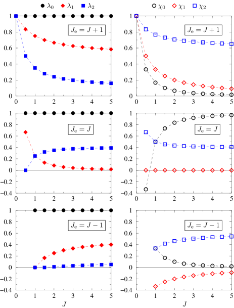
Figure 2: Irreducible eigenvalues of the atomic intensity vertex as a function of the ground-state angular momentum $J$. Left: ladder eigenvalues (46bm). Right: crossed eigenvalues (46bp). The unit ladder eigenvalue $\lambda_{0}=1$ reflects energy conservation. For $J>0$, antisymmetric and symmetric traceless modes are not conserved $\lambda_{1,2}<1$, reflecting depolarization. The crossed scalar eigenvalue $\chi_{0}$ plunges rapidly for $J>0$, $J_{\mathrm{e}}=J+1$, implying a drastic loss of interference contrast. In the semi-classical limit $J_{\mathrm{e}}=J\to\infty$, the interference is re-established since $\chi_{0}\to 1$.

The direct product of two polarization vectors has nine independent components. The atomic scattering vertices therefore can be represented by $9\times 9$ transfer matrices whose eigenvalues are $\lambda_{K}$ and $\chi_{K}$. Since the atomic scattering vertices are averages over a scalar density matrix and therefore invariant under rotations, these eigenvalues are $(2K+1)$-times degenerate (corresponding to the Clebsch-Gordan decomposition of the direct product of representations of dimension $3\times 3=1+3+5$). Introducing the irreducible components greatly simplifies a problem that at first glance defied an analytical treatment. It is thus natural to apply this strategy to the problem of transverse propagation as well.

5.3 Irreducible eigenmodes of the transverse intensity propagator

The sum over the polarizations of an intermediate photon in scattering diagrams like (42) defines a transverse projector $\sum_{\boldsymbol{\varepsilon}\perp\bi k}\varepsilon_{i}\bar{\varepsilon}_{j}=\delta_{ij}-\hat{k}_{i}\hat{k}_{j}$. The average retarded propagator for the transverse field in momentum space therefore can be written

$$\left\langle G_{ij}(k;\omega)\right\rangle=\frac{\delta_{ij}-\hat{k}_{i}\hat{k}_{j}}{\omega-k-\Sigma(\omega)}.$$ (46bq)

Up to near-field terms, the average real-space propagator is given by (cf. (46ax))

$$\left\langle G_{ij}(r;\omega)\right\rangle=-\frac{\omega}{2\pi r}\,\rme^{\rmi(k-\Sigma(\omega))r}\Delta_{ij}$$ (46br)

where $\Delta_{ij}=\delta_{ij}-\hat{r}_{i}\hat{r}_{j}$ is the projector onto the plane transverse to the direction of propagation. Generalizing the scalar case (46ay), we now need to analyze the transverse intensity propagator between scattering events,

$$\mathsf{G}_{il;jk}(\bi q)=\frac{3}{8\pi\ell}\int{\mathrm{d}}^{3}r\,\frac{\rme^{-r/\ell}}{r^{2}}\,\Delta_{ij}\Delta_{kl}\,\rme^{\rmi\bi{q}\cdot\bi{r}}.$$ (46bs)

Here, the prefactor $u(\omega,0)=3n\sigma/(4\pi\rho_{0}(\omega))$ from the atomic vertex has been incorporated in order to manipulate a dimensionless quantity. All information on the vector character is contained in the direct product $\Delta_{ij}\Delta_{kl}$ of transverse projectors. Contrary to the rotation-invariant atomic vertex, the intensity propagator now depends on the momentum $\bi q$. Thus isotropic tensor modes can no longer be sufficient, leading to a more involved, but still exact decomposition (for details, see A)

$$\mathsf{G}_{il;jk}(\bi q)=\hat{s}_{2}(p)\,P_{ij}P_{kl}+\hat{s}_{1}(p)\,[P_{ij}Q_{kl}+Q_{ij}P_{kl}]+8\hat{s}_{3}(p)\;Q_{ij}Q_{kl}$$

$$+\hat{s}_{3}(p)\;[P_{ij}P_{kl}+2\,\mathrm{perm.}]+\hat{s}_{4}(p)\;[P_{ij}Q_{kl}+5\,\mathrm{perm.}]$$ (46bt)

in terms of the projectors $Q_{ij}=\hat{q}_{i}\hat{q}_{j}$ and $P_{ij}=\delta_{ij}-Q_{ij}$ onto the direction $\hat{\bi}{q}=\bi q/q$ and the plane perpendicular to it. Indeed, the projectors $Q_{ij}$ and $P_{ij}$ are the natural objects to deal with transversality and yield the most concise expressions. The terms in the second line of the right hand side of (46bt) are totally symmetric with respect to any permutation of indices which is indicated by “$+n\,\mathrm{perm.}$”. The functions $\hat{s}_{\alpha}(p)$ are given in equations (46dn) and (46dw) of the appendix; $p=q\ell$ is the reduced momentum. The transverse projector in real space $\Delta_{ij}\Delta_{kl}$ has the very simple structure of a direct product which is obviously not conserved by the Fourier transformation. In momentum space, the (difficult) real-space integral equation of multiple scattering becomes a (simple) geometrical series of diagonal operators, but the price to be paid is the complicated coupling between momentum and polarization expressed by (46bt).

Analyzing (46bt) in irreducible left-right components $\mathsf{G}^{(K,K^{\prime})}=\mathsf{T}^{(K)}\mathsf{G}\mathsf{T}^{(K^{\prime})}$ as described in A, the transverse intensity propagator takes the form

$$\mathsf{G}(\bi q)=\sum_{K,\alpha}g_{K\alpha}(p)\;\mathsf{T}^{(K)}_{\alpha}(\hat{\bi}{q})+\tilde{g}(p)\left(\mathsf{\widetilde{T}}^{(0,2)}(\hat{\bi}{q})+\mathsf{\widetilde{T}}^{(2,0)}(\hat{\bi}{q})\right).$$ (46bu)

The nine $p$-dependent eigenvalues of the $9\times 9$ transfer matrix are partially degenerate such that only six irreducible eigenvalues are relevant,

$$\eqalign{g_{00}(p)&\equiv\mathcal{A}(p)=\frac{\arctan(p)}{p}=1-\frac{p^{2}}{3}+O(p^{4}),\\ g_{11}(p)&=\frac{3\left(1-\mathcal{A}(p)\right)}{2p^{2}}=\frac{1}{2}-\frac{3p^{2}}{10}+O(p^{4}),\\ g_{12}(p)&=\frac{3\left(-1+(1+p^{2})\mathcal{A}(p)\right)}{4p^{2}}=\frac{1}{2}-\frac{p^{2}}{10}+O(p^{4}),\\ g_{20}(p)&=\frac{-9(1+p^{2})+(9+12p^{4}+5p^{4})\mathcal{A}(p)}{4p^{4}}=\frac{7}{10}-\frac{29p^{2}}{210}+O(p^{4}),\\ g_{21}(p)&=\frac{6+p^{2}-3(2+p^{2}-p^{4})\mathcal{A}(p)}{4p^{4}}=\frac{7}{10}-\frac{13p^{2}}{70}+O(p^{4}),\\ g_{22}(p)&=\frac{-3+7p^{2}+3(1-p^{2})^{2}\mathcal{A}(p)}{8p^{4}}=\frac{7}{10}-\frac{23p^{2}}{70}+O(p^{4}).}$$ (46bv)

Figure 3: Irreducible eigenvalues (46bv) of the transverse intensity propagator as functions of the reduced moment $p=q\ell$. At the isotropic limit $p=0$, the eigenvalues are $(2K+1)$-fold degenerate, and the coupling $\tilde{g}(p)$, equation (46bx), between scalar and symmetric traceless modes vanishes.

The $(2K+1)$-degenerate eigenvalues at the origin, $g_{K\alpha}(0)$, have been used by Akkermans et al. [6] in a qualitative evaluation of polarization effects on the coherent backscattering peak, based on the diffusion approximation for scalar waves. The expressions at order $p^{2}$ (with a small error for the coefficient of $g_{20}$) have been found by Stephen and Cwilich [35, (7.4)–(4.9)] and MacKintosh and John [36, (4.16)]. The above functions, noted $\lambda_{i}(p)=1-g_{K\alpha}(p)$, are identical to those found by Ozrin [18, (3.16)]. In a slightly modified form, they appear also in the radiative transfer theory solved exactly by Amic, Luc and Nieuwenhuizen [19, (3.8),(3.15)]. But these last approaches do not make use of an explicit analysis in terms of irreducible components, which here gives also the projectors on the corresponding eigenmodes in terms of $P_{ij}=\delta_{ij}-\hat{q}_{i}\hat{q}_{j}$ and $Q_{ij}=\hat{q}_{i}\hat{q}_{j}$:

$$\eqalign{\mathsf{T}^{(0)}_{0,il;jk}&\equiv\frac{1}{3}\,\delta_{il}\delta_{jk},\\ \mathsf{T}^{(1)}_{1}(\hat{\bi}{q})_{il;jk}&=\frac{1}{2}(P_{ij}P_{kl}-P_{ik}P_{jl}),\\ \mathsf{T}^{(1)}_{2}(\hat{\bi}{q})_{il;jk}&=\frac{1}{2}(P_{ij}Q_{kl}+Q_{ij}P_{kl}-P_{ik}Q_{jl}-Q_{ik}P_{jl}),\\ \mathsf{T}^{(2)}_{0}(\hat{\bi}{q})_{il;jk}&=\frac{1}{6}(P_{il}-2Q_{il})(P_{jk}-2Q_{jk}),\\ \mathsf{T}^{(2)}_{1}(\hat{\bi}{q})_{il;jk}&=\frac{1}{2}(P_{ij}Q_{kl}+Q_{ij}P_{kl}+P_{ik}Q_{jl}+Q_{ik}P_{jl}),\\ \mathsf{T}^{(2)}_{2}(\hat{\bi}{q})_{il;jk}&=\frac{1}{2}(P_{ij}P_{kl}+P_{ik}P_{jl})-\frac{1}{2}P_{il}P_{jk}.}$$ (46bw)

For the “horizontal” tensor product (46bc), the above tensors are orthogonal projectors, $\mathsf{T}^{(K)}_{\alpha}\mathsf{T}^{(K^{\prime})}_{\beta}=\delta_{KK^{\prime}}\delta_{\alpha\beta}\mathsf{T}^{(K)}_{\alpha}$. At the limit $\bi q=0$, they recombine to give the isotropic tensors (46bh) encountered in the decomposition of the rotation-invariant atomic vertex, $\sum_{\alpha}\mathsf{T}^{(K)}_{\alpha}(\hat{\bi}{q})=\mathsf{T}^{(K)}$. But this decomposition does not yield a totally diagonal representation. As already pointed out by Ozrin [18], there exists an irreducible coupling term between the scalar and one symmetric traceless mode that vanishes at the origin,

$$\tilde{g}(p)=\frac{\sqrt{2}[3-(3+p^{2})\mathcal{A}(p)]}{4p^{2}}=-\frac{\sqrt{2}\,p^{2}}{15}+O(p^{4})$$ (46bx)

with coupling tensors

$$\mathsf{\widetilde{T}}^{(0,2)}(\hat{\bi}{q})_{il;jk}=\frac{\sqrt{2}}{6}\;\delta_{il}\;(P_{jk}-2Q_{jk}),\qquad\mathsf{\widetilde{T}}^{(2,0)}(\hat{\bi}{q})_{il;jk}=\frac{\sqrt{2}}{6}\;(P_{il}-2Q_{il})\;\delta_{jk}.$$ (46by)

The multiplication table (46ee) of these coupling tensors can be found in the appendix. This coupling at $\bi q\neq 0$ can of course be formally diagonalized, at the price of rather unwieldy expressions. At the limit of the summed multiple scattering series, this coupling term is more simply taken care of by the diagonalization of a $2\times 2$ matrix. Furthermore, it vanishes in the diffusion approximation.

5.4 Sum of the ladder and crossed series

The tensor $\mathsf{A}$ entering into the ladder series (46az) is given as the product of transverse intensity propagator and atomic intensity vertex, $\mathsf{A}_{L}(\bi q)\equiv\mathsf{G}(\bi q)\,\mathsf{I}$. Knowing the respective decompositions (46bi) and (46bu) into eigenmodes, the product is simply

$$\mathsf{A}_{L}(\bi q)=\sum_{K,\alpha}\lambda_{K}g_{K\alpha}(p)\,\mathsf{T}^{(K)}_{\alpha}+\lambda_{2}\tilde{g}(p)\mathsf{\widetilde{T}}^{(0,2)}+\lambda_{0}\tilde{g}(p)\mathsf{\widetilde{T}}^{(2,0)}.$$ (46bz)

The message of this expression is clear: in order to generalize the multiple scattering of light to atoms, it suffices to multiply the vector eigenfunctions $g_{K\alpha}(p)$ by the corresponding atomic eigenvalue $\lambda_{K}(J,J_{\mathrm{e}})$ — a rather trivial prescription once the meaning of the word “corresponding” has been clarified (which constitutes the main achievement of the present theory).

The sum of all ladder diagrams is $\mathsf{L}(\bi q)=\mathsf{I}\,(\mathsf{1}-\mathsf{A}_{L}(\bi q))^{-1}$. To invert $(\mathsf{1}-\mathsf{A}_{L}(\bi q))$, we try the Ansatz

$$(\mathsf{1}-\mathsf{A}_{L})^{-1}=\sum_{K,\alpha}a_{K\alpha}\,\mathsf{T}^{(K)}_{\alpha}+\tilde{a}_{2}\mathsf{\widetilde{T}}^{(0,2)}+\tilde{a}_{0}\mathsf{\widetilde{T}}^{(2,0)}.$$ (46ca)

By definition, $(\mathsf{1}-\mathsf{A}_{L}(\bi q))(\mathsf{1}-\mathsf{A}_{L}(\bi q))^{-1}=\mathsf{1}$. The identity being $\mathsf{1}=\sum_{K,\alpha}\mathsf{T}^{(K)}_{\alpha}$, the coefficients of (46ca) are completely determined. For the decoupled modes, i.e. all except $(K=0,2,\,\alpha=0)$, the result simply is $a_{K\alpha}=(1-\lambda_{K}g_{K\alpha})^{-1}$. The coefficients for the coupled modes are determined by two independent linear systems,

$$\left(\begin{array}[]{c}a_{00}\\ \tilde{a}_{0}\end{array}\right)=\boldsymbol{\Lambda}^{-1}\left(\begin{array}[]{c}1\\ 0\end{array}\right),\qquad\left(\begin{array}[]{c}\tilde{a}_{2}\\ a_{20}\end{array}\right)=\boldsymbol{\Lambda}^{-1}\left(\begin{array}[]{c}0\\ 1\end{array}\right).$$ (46cb)

Here, the $2\times 2$ coupling matrix is

$$\boldsymbol{\Lambda}\equiv\left(\begin{array}[]{cc}1-\lambda_{0}g_{00}&-\lambda_{2}\tilde{g}\\ -\lambda_{0}\tilde{g}&1-\lambda_{2}g_{20}\end{array}\right),$$ (46cc)

with determinant $|\Lambda|\equiv(1-\lambda_{0}g_{00})(1-\lambda_{2}g_{20})-\lambda_{0}\lambda_{2}\tilde{g}^{2}$. The coefficients of the summed series are therefore obtained by inverting this matrix, yielding

$$a_{00}=\frac{1-\lambda_{2}g_{20}}{|\Lambda|},\quad a_{20}=\frac{1-\lambda_{0}g_{00}}{|\Lambda|},\quad\tilde{a}_{0}=\frac{\lambda_{0}\tilde{g}}{|\Lambda|},\quad\tilde{a}_{2}=\frac{\lambda_{2}\tilde{g}}{|\Lambda|}.$$ (46cd)

Regrouping all terms, we obtain the summed ladder series as

$$\mathsf{L}(\bi q)=\sum_{K,\alpha}\Lambda_{K\alpha}(p)\mathsf{T}^{(K)}_{\alpha}(\hat{\bi}{q})+\widetilde{\Lambda}(p)\widetilde{\mathsf{T}}(\hat{\bi}{q})$$ (46ce)

where the coefficients are

$$\eqalign{\Lambda_{00}\equiv\lambda_{0}\frac{1-\lambda_{2}g_{20}}{|\Lambda|},\qquad\Lambda_{11}\equiv\frac{\lambda_{1}}{1-\lambda_{1}g_{11}},\qquad\Lambda_{12}\equiv\frac{\lambda_{1}}{1-\lambda_{1}g_{12}},\\ \Lambda_{20}\equiv\lambda_{2}\frac{1-\lambda_{0}g_{00}}{|\Lambda|},\qquad\Lambda_{21}\equiv\frac{\lambda_{2}}{1-\lambda_{2}g_{21}},\qquad\Lambda_{22}\equiv\frac{\lambda_{2}}{1-\lambda_{2}g_{22}},}$$ (46cf)

in terms of the atomic ladder eigenvalues $\lambda_{K}(J,J_{\mathrm{e}})$ defined in (46bm) and the eigenfunctions $g_{K\alpha}(p)$ of transverse propagation (equations (46bv)). The tensors $\mathsf{T}^{(K)}_{\alpha}(\hat{\bi}{q})$ carrying the information about the angular dependence have been defined in (46bw). The irreducible coupling term

$$\widetilde{\Lambda}(p)\equiv\lambda_{2}\lambda_{0}\frac{\tilde{g}(p)}{|\Lambda|}$$ (46cg)

is proportional to the coupling function (46bx) which vanishes as $p\to 0$. Its associated tensor is $\widetilde{\mathsf{T}}(\hat{\bi}{q})\equiv\widetilde{\mathsf{T}}^{(2,0)}(\hat{\bi}{q})+\widetilde{\mathsf{T}}^{(0,2)}(\hat{\bi}{q})$ in terms of the left and right coupling tensors given in (46by).

Finally, we have to contract the external polarization vectors with the tensors, yielding the weights of the different field modes,

$$\eqalign{t^{(K)}_{L,\alpha}(\hat{\bi}{q})&\equiv\varepsilon_{1,i}\,\bar{\varepsilon}_{2,j}\,\varepsilon_{3,k}\,\bar{\varepsilon}_{4,l}\,\mathsf{T}^{(K)}_{\alpha}(\hat{\bi}{q})_{il;jk},\\ \tilde{t}_{L}(\hat{\bi}{q})&\equiv\varepsilon_{1,i}\,\bar{\varepsilon}_{2,j}\,\varepsilon_{3,k}\,\bar{\varepsilon}_{4,l}\,\mathsf{\widetilde{T}}(\hat{\bi}{q})_{il;jk}.}$$ (46ch)

Here, the populations of the different field modes are determined by the choice of polarization, and are in particular independent of the atomic internal structure which enters only in the corresponding propagators $\Lambda(p;J)$. The summed transverse atomic ladder propagator in momentum space reads

$$L(\bi q)\equiv u(\omega)\Big{(}\sum_{K,\alpha}\Lambda_{K\alpha}(p)\,t^{(K)}_{L,\alpha}(\hat{\bi}{q})+\widetilde{\Lambda}(p)\,\tilde{t}_{L}(\hat{\bi}{q})\Big{)}.$$ (46ci)

Proceeding similarly, one obtains the summed crossed tensor

$$\mathsf{C}(\bi q)=\sum_{K,\alpha}X_{K\alpha}(p)\mathsf{T}^{(K)}_{\alpha}(\hat{\bi}{q})+\widetilde{X}(p)\mathsf{\widetilde{T}}(\hat{\bi}{q}).$$ (46cj)

The same tensors as for the ladder series appear, and the coefficients are obtained by substracting the single-scattering contribution and replacing the atomic ladder eigenvalues $\lambda_{K}$ by the corresponding crossed eigenvalues $\chi_{K}$,

$$\eqalign{X_{00}\equiv\chi_{0}\left(\frac{1-\chi_{2}g_{20}}{|X|}-1\right),\qquad X_{11}\equiv\frac{\chi_{1}^{2}g_{11}}{1-\chi_{1}g_{11}},\qquad X_{12}\equiv\frac{\chi_{1}^{2}g_{12}}{1-\chi_{1}g_{12}},\\ X_{20}\equiv\chi_{2}\left(\frac{1-\chi_{0}g_{00}}{|X|}-1\right),\qquad X_{21}\equiv\frac{\chi_{2}^{2}g_{21}}{1-\chi_{2}g_{21}},\qquad X_{22}\equiv\frac{\chi_{2}^{2}g_{22}}{1-\chi_{2}g_{22}}.}$$ (46ck)

The determinant of the crossed coupling matrix is $|X|\equiv(1-\chi_{0}g_{00})(1-\chi_{2}g_{20})-\chi_{0}\chi_{2}\tilde{g}^{2}$. The coupling coefficient reads accordingly

$$\widetilde{X}(p)\equiv\chi_{2}\chi_{0}\frac{\tilde{g}(p)}{|X|}$$ (46cl)

The eigenvalues $\chi_{K}(J,J_{\mathrm{e}})$ of the twisted atomic intensity vertex have been defined in equation (46bp). The weights of the different modes are determined by contracting the tensors with the external polarization vectors (respecting the substitution rule (46b)):

$$\eqalign{t^{(K)}_{C,\alpha}(\hat{\bi}{q})&\equiv\varepsilon_{1,i}\,\bar{\varepsilon}_{2,j}\,\bar{\varepsilon}_{4,k}\,\varepsilon_{3,l}\,\mathsf{T}^{(K)}_{\alpha}(\hat{\bi}{q})_{il;jk},\\ \tilde{t}_{C}(\hat{\bi}{q})&\equiv\varepsilon_{1,i}\,\bar{\varepsilon}_{2,j}\,\bar{\varepsilon}_{4,k}\,\varepsilon_{3,l}\,\mathsf{\widetilde{T}}(\hat{\bi}{q})_{il;jk}.}$$ (46cm)

As for the ladder case, the population of a field mode is determined solely by the choice of polarization vectors (but is different from the corresponding ladder mode unless $\boldsymbol{\bar{\varepsilon}}_{4}=\boldsymbol{\varepsilon}_{3}$). The atomic internal structure only enters in the corresponding propagators $X(p;J)$. The total summed crossed propagator therefore reads

$$C(\bi q)\equiv u(\omega)\Big{(}\sum_{K,\alpha}X_{K\alpha}(p)\,t^{(K)}_{C,\alpha}(\hat{\bi}{q})+\widetilde{X}(p)\,\tilde{t}_{C}(\hat{\bi}{q})\Big{)}.$$ (46cn)

6 Transport velocity, diffusion constant and relaxation times

Let us now turn to the discussion of dynamic quantities like the transport velocity and the diffusion constant for the different field modes. In the dynamic setting $\Omega\neq 0$, the atomic ladder and crossed vertices (46bi) and (46bn) remain unchanged. Indeed, the only dependence on frequency had been factorized in the prefactor $u(\omega,\Omega)=NM_{J}t(\omega_{+})\bar{t}(\omega_{-})$ and included in the transverse ladder kernel (46bs),

$$\mathsf{G}_{il;jk}(\bi q,\Omega)=u(\omega,\Omega)L^{3}\int\rmd^{3}r\left\langle G_{ij}(\bi r;\omega_{+})\right\rangle\left\langle\overline{G}_{kl}(\bi r;\omega_{-})\right\rangle\rme^{\rmi\bi q\cdot\bi r}$$ (46co)

where $\omega_{\pm}=\omega\pm\Omega/2$. Then,

$$\mathsf{G}_{il;jk}(\bi q,\Omega)=\mathcal{B}(\Omega)\frac{3}{8\pi\ell(\Omega)}\int{\mathrm{d}}^{3}r\,\frac{\rme^{-r/\ell(\Omega)}}{r^{2}}\,\Delta_{ij}\Delta_{kl}\,\rme^{\rmi\bi{q}\cdot\bi{r}}$$ (46cp)

where the frequency dependence of the propagators gives rise to an $\Omega$-dependent complex scattering mean free path

$$\ell(\Omega)=\frac{1}{\rmi\Sigma(\omega_{+})-\rmi\overline{\Sigma}(\omega_{-})-\rmi\Omega}.$$ (46cq)

The static limit is of course $\ell(0)=\ell=-1/2\mathrm{Im}\,\Sigma(\omega)$. Using $\Sigma(\omega)=NM_{J}t(\omega)$, the prefactor of the integral (46cp) can be written

$$\mathcal{B}(\Omega)=\frac{\Sigma(\omega_{+})\overline{\Sigma}(\omega_{-})}{|\Sigma(\omega)|^{2}}\frac{\ell(\Omega)}{\ell}$$ (46cr)

such that $\mathcal{B}(0)=1$. Obviously, the tensor structure and $\bi q$-dependence in (46cp) are identical to the static case (46bs), so that the Fourier-Laplace transforms yield the same results, now featuring the complex mean free path $\ell(\Omega)$. The eigenfunctions of the transverse propagator become

$$g_{K\alpha}(q,\Omega)=\mathcal{B}(\Omega)g_{K\alpha}(p(\Omega)),$$ (46cs)

where the static eigenfunctions $g_{K\alpha}(p)$, given in (46bv), are evaluated at the dynamic reduced moment $p(\Omega)=q\ell(\Omega)$. Since the atomic eigenvalues $\lambda_{K}$ and $\chi_{K}$ are not affected, the ladder and crossed sums are still given by (46ci) and (46cn), with the dynamic eigenfunctions (46cs) and the dynamic prefactor $u(\omega,\Omega)$. Please note that these expressions are exact in $\Omega$ and $q$.

6.1 Transport velocity

In order to determine the long-time and long-distance behaviour of transport, one habitually develops the propagator to lowest orders in $\Omega$ and $q$. Since the atomic internal structure has completely factorized from the frequency dependence, we exactly recover results that are well-known from the case of resonant scattering of scalar waves by point particles [23, 25]. Let us briefly show how the main results are obtained very easily in our framework. The small frequency behavior of (46cr), $\mathcal{B}(\Omega)=1+\rmi\Omega\tau_{\mathrm{tr}}+O(\Omega^{2})$, defines a common transport time scale for all field modes,

$$\tau_{\mathrm{tr}}=\mathrm{Im}\,\frac{\Sigma^{\prime}(\omega)}{\Sigma(\omega)}+\ell(1-\mathrm{Re}\,\Sigma^{\prime}(\omega)).$$ (46ct)

where $\Sigma^{\prime}=\rmd\Sigma/\rmd\omega$. Its two contributions have simple physical interpretations. The first term on the right-hand side can be traced back to the prefactor $u(\omega,\Omega)$ and is simply the (Wigner) time delay

$$\tau_{\mathrm{W}}=\mathrm{Im}\,\frac{\Sigma^{\prime}(\omega)}{\Sigma(\omega)}=\frac{\rmd\phi(\omega)}{\rmd\omega}$$ (46cu)

where $\phi(\omega)$ is the phase of the scattering t-matrix $t(\omega)=\Sigma(\omega)/NM_{J}$. The second term is the propagation time $\ell/v_{\mathrm{g}}$ between consecutive scatterering events with the group velocity inside the effective medium, $v_{\mathrm{g}}=\rmd\omega/\rmd k=(1-\mathrm{Re}\,\Sigma^{\prime}(\omega))^{-1}$ (remember $c=1$ and the real part of the dispersion relation, $k(\omega)=\omega-\mathrm{Re}\,\Sigma(\omega)$). The group velocity by itself looses its physical meaning in the vicinity of a scattering resonance where extinction cannot be neglected. The transport velocity $v_{\mathrm{tr}}=\ell/\tau_{\mathrm{tr}}=(v_{\mathrm{g}}^{-1}+\tau_{\mathrm{W}})^{-1}$, however, stays causal, $v_{\mathrm{tr}}\leq 1$, at all frequencies $\omega$, and may decrease by orders of magnitude at resonance for a high enough density of scatterers [39, 23]. In the present case of resonant point scatterers, the above expressions simplify remarkably since

$$\frac{\mathrm{Re}\,\Sigma^{\prime}(\omega)}{2\mathrm{Im}\,\Sigma(\omega)}+\mathrm{Im}\,\frac{\Sigma^{\prime}(\omega)}{\Sigma(\omega)}=\frac{1}{\Gamma},$$ (46cv)

up to terms of order $(\delta/\omega)^{2},(\Gamma/\omega)^{2}$. The transport velocity then takes the simple form $v_{\mathrm{tr}}=(1+(\Gamma\ell)^{-1})^{-1}$, which corresponds to an inverted Lorentzian of width $\Gamma$ because of the resonant character of the inverse scattering mean free path $\ell^{-1}\propto 1/(\delta^{2}+\Gamma^{2}/4)$. The sum (46cv) has been called “dwell time” (in the case of non-resonant ($\Gamma\to\infty$) scattering of electrons, the dwell time vanishes due to a Ward identity that is invalid for scattering by frequency-dependent potentials [39]). The total time of transport (46ct) can be written as the sum of the free propagation time $\ell$ between consecutive scatterers and the dwell time $1/\Gamma$. At resonance, for example, the Wigner time delay is $\tau_{\mathrm{W}}=2/\Gamma$, but the group velocity correction is negative since $\mathrm{Re}\,\Sigma^{\prime}(\omega_{0})/2\mathrm{Im}\,\Sigma(\omega_{0})=-1/\Gamma$. Whereas the Wigner time delay accounts for the (possibly large time) spent “inside” a resonant scattering object, the total dwell time includes the self-consistent dressing of scatterers by the surrounding effective medium which must not be neglected.

6.2 Extinction lengths

The transversality of the light field and the atomic internal structure are connected to the spatial variable $\bi q$. Setting $\Omega=0$ in a first step, all propagation eigenfunctions (46bv) have a quadratic development in $p=q\ell$ of the form $g_{K\alpha}(p)\approx b_{K}-c_{K\alpha}p^{2}$, whereas the coupling term vanishes quadratically, $\tilde{g}(p)=\tilde{c}p^{2}$. At order $p^{2}$, the coupling between scalar and symmetric traceless modes disappears, and the propagators (46cf) for the transverse ladder modes behave like

$$\Lambda_{K\alpha}(p)\approx\frac{\lambda_{K}}{1-\lambda_{K}(b_{K}-c_{K\alpha}p^{2})}=\frac{c_{K\alpha}^{-1}\ell^{-2}}{q^{2}+\ell^{-2}_{K\alpha}}.$$ (46cw)

Here appears an extinction length

$$\ell_{K\alpha}(J)=\ell\sqrt{\frac{c_{K\alpha}}{\lambda_{K}^{-1}-b_{K}}}$$ (46cx)

that is responsible for an exponential decay of the mode $K,\alpha$ in real-space (in field theory, this corresponds to a finite particle mass $m=\ell^{-1}_{K\alpha}$). We notice immediately that the intensity or scalar mode $K=0$ has a diverging extinction length since $b_{0}=1$ and $\lambda_{0}=1$ for arbitrary internal degeneracy. This true diffusion pole (or massless Goldstone mode) survives thanks to a fundamental conservation law, the conservation of energy. All other field modes have finite, and in fact rather short extinction lengths $\ell_{K\alpha}(J)\lesssim\ell$, implying that the transversality of propagation mixes well-defined polarization modes. The smaller $b_{K}$ and $\lambda_{K}$, the shorter the extinction length. Thus, the atomic internal degeneracy, responsible for $\lambda_{1,2}<1$ as soon as $J>0$, leads to even smaller extinction lengths for non-scalar field modes. This observation confirms the intuitive picture that degenerate Raman transitions between different Zeeman sublevels $|Jm^{\prime}\rangle\neq|Jm\rangle$ contribute to scramble the field polarization.

Analogous arguments apply for the crossed propagator. Here, the atomic ladder eigenvalues are replaced by their crossed counterparts $\chi_{K}$, and the crossed extinction lengths are

$$\xi_{K\alpha}(J)=\ell\sqrt{\frac{c_{K\alpha}}{\chi_{K}^{-1}-b_{K}}}.$$ (46cy)

The scalar eigenvalue $\chi_{0}$ is not constrained by energy conservation and can become very small for $J>0$ (cf. figure 2). The atomic internal degeneracy breaks the time-reversal symmetry between ladder and crossed propagators, and leads to a rapid exponential damping of the interference modes.

Extinctions lengths of the order of or smaller than the scattering mean free path $\ell$ imply that the evolution can no longer be considered diffusive. Amic et al. [19] have stressed that the exact extinction length, defined as the inverse of the pole of the propagator with smallest imaginary real part, can differ from the above diffusive expression by as much as $50\%$. This difference is bound to become even worse as the atomic eigenvalues decreases. Clearly, a quantitative prediction for the propagation of the full vector field must go beyond the diffusion approximation. This is especially true if one is interested in coherent backscattering from a finite scattering medium, where short paths or non-scalar field modes can become dominant.

6.3 Diffusion constant and relaxation times

Combining the developments linear in $\Omega$ and quadratic in $q$, the ladder propagators take the form

$$\Lambda_{K\alpha}(q,\Omega)\approx\frac{(b_{K}\tau_{\mathrm{tr}})^{-1}}{-\rmi\Omega+t_{K}^{-1}+D_{K\alpha}q^{2}}.$$ (46cz)

Here appears the diffusion constant $D_{K\alpha}=(3c_{K\alpha}/b_{K})\,D_{0}$ for the corresponding field mode, simply proportional to the diffusion constant of the intensity, $D_{0}=\ell v_{\mathrm{tr}}/3$, and independent of the atomic eigenvalues. Furthermore, a relaxation time has been defined,

$$t_{K}=\frac{\tau_{\mathrm{tr}}}{(\lambda_{K}b_{K})^{-1}-1}$$ (46da)

The physical meaning of this relaxation time is equivalent to that of the extinction lengths $\ell_{K\alpha}$ defined above since $\ell_{K\alpha}^{2}=D_{K\alpha}t_{K}$. For the scalar mode of field intensity, $t_{0}^{-1}=0$ implies a truly diffusive transport as required by local energy conservation. For the non-scalar field modes, the finite relaxation times $t_{1,2}$ become of the order of the transport time $\tau_{\mathrm{tr}}$ indicating that light transport can no longer be described accurately in the diffusion approximation, a tendency aggravated by the internal atomic degeneracy leading to $\lambda_{1,2}<1$. For the crossed propagator, analogous conclusions hold. The quantum internal structure introduces dephasing times as will be discussed elsewhere [40].

6.4 Conclusion and things to be done

In summary, we develop a consistent theory for the multiple scattering of photons by a dilute gas of cold atoms. The external degrees of freedom of the atomic point scatterers are supposed to be classical Poissonian variables. Particular attention is paid to the internal degrees of freedom: a resonant dipole transition of arbitrary degeneracy is treated analytically by a systematic use of irreducible tensor operators. We sum the ladder diagrams of the full transverse vector field, and calculate the correction of maximally crossed diagrams. The internal degeneracy has no impact on the properties of the average amplitude (such as the scattering mean free path) since the average over a scalar internal density matrix projects onto the scalar component of the transition matrix. Furthermore, the internal degeneracy is only coupled to the (static) polarization vectors and completely factorized from the (dynamic) frequency dependence. Therefore, the transport velocity and the diffusion constant remain unaffected. However, the interference properties are strongly modified. Indeed, the non-scalar parts of the scattering t-matrix survive in the average intensity and are responsible for a decrease of contrast as soon as $J>0$. In the diffusion approximation, we give expressions for extinction lengths or relaxation times that depend in very simple manner on $J$. Atoms thus appear as an important class of anisotropic scatterers with intriguing interference properties that allow a complete analytical description of light scattering.

The present contribution deals with transport inside an infinite scattering medium, taking full advantage of the statistical invariance under translations which makes all operators diagonal in momentum representation. The influence of boundary conditions, relevant for coherent backscattering or transmission experiments, may be evaluated in the framework of the exact Wiener-Hopf method or of the approximate method of images. Both approaches deserve a detailed discussion which is beyond the scope of this paper and will be discussed elsewhere [41]. Another important issue is the influence of an external magnetic field. Perhaps the systematic use of irreducible tensors can help to simplify the theoretical description of light transport in magneto-active media [42]. In addition, the impact of a splitting of the internal Zeeman degeneracy remains to be studied, experimentally as well as theoretically.

The transversality of the propagating light field imposes a change of polarization in the course of multiple scattering. In this respect, the present theory provides a microscopic analogue of spin-orbit coupling studied extensively in electronic disordered systems [8]. But contrary to the electron case of spin $\frac{1}{2}$, no weak anti-localization for the spin $1$ photon can be expected, however strong the spin-orbit coupling. The scattering of photons by atoms with internal degeneracy appears as an analogue of spin-flip scattering of electrons by magnetic impurities [8]. Interestingly, we can derive exact expressions for characteristic extinction lengths and relaxation times, and further experimental as well as theoretical studies can be envisaged. The links between optics and atomic physics on the one hand and condensed matter physics on the other thus promise to continue to be an important source of inspiration to both fields.

Appendix A How to find the irreducible eigenmodes of the transverse intensity propagator

A.1 Decomposition in real space

Starting from the purely transverse projector in real space $\mathsf{G}_{il;jk}(\hat{\bi}{r})\equiv\Delta_{ij}\Delta_{kl}$, where $\Delta_{ij}=\delta_{ij}-\hat{r}_{i}\hat{r}_{j}$, let us first determine its “left” and “right” irreducible components by projecting onto the isotropic basis tensors (46bh),

$$\mathsf{G}^{(K,K^{\prime})}(\hat{\bi}{r})\equiv\mathsf{T}^{(K)}\mathsf{G}(\hat{\bi}{r})\mathsf{T}^{(K^{\prime})}.$$ (46db)

The exchange symmetry $(i,j)\leftrightarrow(l,k)$ implies that the sum of orders $K+K^{\prime}$ is even since $\mathsf{G}_{il;jk}^{(K,K^{\prime})}(\hat{\bi}{r})=\mathsf{G}_{li;kj}^{(K,K^{\prime})}(\hat{\bi}{r})=(-1)^{K+K^{\prime}}\mathsf{G}_{il;jk}^{(K,K^{\prime})}(\hat{\bi}{r})$, by parity properties of the $\mathsf{T}^{(K)}$. This condition decouples the antisymmetric from the symmetric modes. We find the purely scalar component

$$\mathsf{G}_{il;jk}^{(0,0)}(\hat{\bi}{r})=\frac{2}{9}\,\delta_{il}\delta_{jk},$$ (46dc)

the antisymmetric component

$$\mathsf{G}_{il;jk}^{(1,1)}(\hat{\bi}{r})=\frac{1}{2}(\Delta_{ij}\Delta_{kl}-\Delta_{ik}\Delta_{jl}),$$ (46dd)

the traceless symmetric component

$$\mathsf{G}_{il;jk}^{(2,2)}(\hat{\bi}{r})=\frac{1}{2}(\Delta_{ij}\Delta_{kl}+\Delta_{ik}\Delta_{jl})-\frac{1}{3}(\delta_{il}\Delta_{jk}+\delta_{jk}\Delta_{il})+\frac{2}{9}\,\delta_{il}\delta_{jk},$$ (46de)

as well as two scalar-symmetric mixed components

$$\mathsf{G}_{il;jk}^{(0,2)}(\hat{\bi}{r})=\frac{1}{9}\,\delta_{il}\,(\Delta_{jk}-2\hat{r}_{j}\hat{r}_{k}),\quad\mathsf{G}_{il;jk}^{(2,0)}(\hat{\bi}{r})=\frac{1}{9}\,(\Delta_{il}-2\hat{r}_{i}\hat{r}_{l})\,\delta_{jk}.$$ (46df)

The irreducible components of the transverse propagator $\mathsf{G}(\bi q)$ are thus given by integrating the previous expressions according to (46bs),

$$\mathsf{G}^{(K,K^{\prime})}(\bi q)=\frac{3}{2\ell}\int_{0}^{\infty}{\mathrm{d}}r\,\rme^{-r/\ell}\int\frac{{\mathrm{d}}^{2}\hat{r}}{4\pi}\,\mathsf{G}^{(K,K^{\prime})}(\hat{\bi}{r})\,\rme^{\rmi\bi{q}\cdot\bi{r}}.$$ (46dg)

We introduce the short-hand notation $\mathsf{G}^{(K,K^{\prime})}(\bi q)\equiv\int_{\bi q}\mathsf{G}^{(K,K^{\prime})}(\hat{\bi}{r})$ for this Fourier-Laplace transform. The angular integral of the expressions (46dc)-(46df) depends on the number of times that the components $\hat{r}_{i}$ of the unit vector appear: we distinguish scalar terms of type $\delta_{ij}\delta_{kl}$, quadratic terms of type $\hat{r}_{i}\hat{r}_{j}\delta_{kl}$ and a quaternary term $\hat{r}_{i}\hat{r}_{j}\hat{r}_{k}\hat{r}_{l}$.

A.2 Scalar component

The angular integral of the scalar terms is trivial, of course, and the result of the Fourier-Laplace transform is

$$\int_{\bi q}1\equiv\hat{s}_{0}(p)=\frac{3}{2}\mathcal{A}(q\ell),$$ (46dh)

proportional to the scalar transfer function $\mathcal{A}(p)=\arctan(p)/p$. The scalar component of the transverse propagator therefore is simply given by

$$\mathsf{G}^{(0,0)}(q)=\mathcal{A}(q\ell)\,\mathsf{T}^{(0)}$$ (46di)

using the definition (46bh) of the scalar basis tensor $\mathsf{T}^{(0)}$. Naturally, the scalar component only depends on the transfer function already known from the purely scalar case.

A.3 Antisymmetric components

The angular integral of the quadratic terms is easily solved using a generating function argument,

$$\int\frac{{\mathrm{d}}^{2}\hat{r}}{4\pi}\,\hat{r}_{i}\hat{r}_{j}\rme^{\rmi\bi{q}\cdot\bi{r}}=-\frac{1}{r^{2}}\frac{\partial^{2}}{\partial q_{i}\partial q_{j}}\frac{\sin(qr)}{qr}.$$ (46dj)

Call for brevity $s(x)\equiv\sin(x)/x$, $x=|\bi x|$, $\bi x\equiv r\bi q$, $\partial_{i}\equiv\partial/\partial x_{i}$, and $s^{\prime}(x)=(\rmd/\rmd x)s(x)$ so that (46dj) evaluates to

$$-\partial^{2}_{ij}s(x)=-s^{\prime\prime}(x)\,\hat{q}_{i}\hat{q}_{j}-\frac{s^{\prime}(x)}{x}\,(\delta_{ij}-\hat{q}_{i}\hat{q}_{j}).$$ (46dk)

The derivation (or equivalent angular integration) generates the quadratic terms $\hat{q}_{i}\hat{q}_{j}$ that could be expected, but also a new term proportional to $\delta_{ij}$. Define the two orthogonal projectors on the subspaces parallel and perpendicular to $\hat{\bi}{q}$, $Q_{ij}\equiv\hat{q}_{i}\hat{q}_{j}$ and $P_{ij}\equiv\delta_{ij}-\hat{q}_{i}\hat{q}_{j}$. They add up to the identity $\delta_{ij}$ and satisfy

$$P_{im}P_{mj}=P_{ij},\quad Q_{im}Q_{mj}=Q_{ij},\quad P_{im}Q_{mj}=Q_{im}P_{mj}=0.$$ (46dl)

The Fourier-Laplace integral of quadratic terms is thus given by

$$\int_{\bi q}\hat{r}_{i}\hat{r}_{j}=\hat{s}_{1}(p)\;P_{ij}+\hat{s}_{2}(p)\;Q_{ij}$$ (46dm)

where the coefficients are

$$\eqalign{\hat{s}_{1}(p)&\equiv-\frac{3}{2p}\int_{0}^{\infty}{\mathrm{d}}x\,\rme^{-x/p}\,\frac{s^{\prime}(x)}{x}=-\frac{3[1-(1+p^{2})\mathcal{A}(p)]}{4p^{2}},\\ \hat{s}_{2}(p)&\equiv-\frac{3}{2p}\int_{0}^{\infty}{\mathrm{d}}x\,\rme^{-x/p}\,s^{\prime\prime}(x)=\frac{3[1-\mathcal{A}(p)]}{2p^{2}}.}$$ (46dn)

The three functions $\hat{s}_{0}(p)$ (defined in (46dh)), $\hat{s}_{1}(p)$ and $\hat{s}_{2}(p)$ are not independent. Indeed, the contraction of indices in the quadratic term (46dm) must reproduce the scalar integral (46dh), so that $\hat{s}_{0}(p)=2\hat{s}_{1}(p)+\hat{s}_{2}(p)$.

The purely antisymmetric component of the transverse propagator (46dd) contains only scalar and quadratic terms, so that the previous results permit to write

$$\mathsf{G}^{(1,1)}(\bi q)=g_{11}(p)\,\mathsf{T}^{(1)}_{1}(\hat{\bi}{q})+g_{12}(p)\,\mathsf{T}^{(1)}_{2}(\hat{\bi}{q}).$$ (46do)

The projectors depend on the direction $\hat{\bi}{q}$,

$$\eqalign{\mathsf{T}^{(1)}_{1}(\hat{\bi}{q})_{il;jk}&\equiv\frac{1}{2}(P_{ij}P_{kl}-P_{ik}P_{jl}),\\ \mathsf{T}^{(1)}_{2}(\hat{\bi}{q})_{il;jk}&\equiv\frac{1}{2}(P_{ij}Q_{kl}+Q_{ij}P_{kl}-P_{ik}Q_{jl}-Q_{ik}P_{jl}).}$$ (46dp)

Thanks to the relations (46dl), they are indeed orthogonal projectors for the horizontal tensor product (46bc), $\mathsf{T}^{(1)}_{\alpha}\mathsf{T}^{(1)}_{\beta}=\delta_{\alpha\beta}\,\mathsf{T}^{(1)}_{\alpha}$. By construction, they are purely antisymmetric from left and right, so that the antisymmetriser $\mathsf{T}^{(1)}$ commutes with them, $\mathsf{T}^{(1)}\mathsf{T}^{(1)}_{\alpha}=\mathsf{T}^{(1)}_{\alpha}=\mathsf{T}^{(1)}_{\alpha}\mathsf{T}^{(1)}$. The eigenvalues of the decomposition (46do) depend on the reduced momentum $p=q\ell$,

$$\eqalign{g_{11}(p)&\equiv\hat{s}_{2}(p)=\frac{3[1-\mathcal{A}(p)]}{2p^{2}},\\ g_{12}(p)&\equiv\frac{\hat{s}_{0}(p)-\hat{s}_{2}(p)}{2}=\frac{3[-1+(1+p^{2})\mathcal{A}(p)]}{4p^{2}}.}$$ (46dq)

It is instructive to consider the limit of zero momentum $\bi q\to 0$, where all dependence on the direction $\hat{\bi}{q}$ must vanish. Both eigenfunctions

$$g_{11}(p)=\frac{1}{2}-\frac{3p^{2}}{10}+O(p^{4}),\qquad g_{12}(p)=\frac{1}{2}-\frac{p^{2}}{10}+O(p^{4}),$$ (46dr)

have the common limit $g_{1\alpha}(0)=\frac{1}{2}$, so that the two $\hat{\bi q}$-dependent tensors recombine to the isotropic antisymmetric projector,

$$\mathsf{T}^{(1)}_{1}(\hat{\bi}{q})_{il;jk}+\mathsf{T}^{(1)}_{2}(\hat{\bi}{q})_{il;jk}=\frac{1}{2}(\delta_{ij}\delta_{kl}-\delta_{ik}\delta_{jl})=\mathsf{T}^{(1)}_{il;jk}.$$ (46ds)

The antisymmetric mode $K=1$ must have three eigenvalues that are degenerate at zero momentum where indeed $g_{1\alpha}(0)=\frac{1}{2}$. At finite momentum $p>0$, the degeneracy is partially lifted, and the two distinct eigenvalues $g_{11}(p)$ and $g_{12}(p)$ appear. Ozrin obtains the same eigenfunctions (noted $1-\lambda_{9}(p)$ and $1-\lambda_{5}(p)$, respectively, [21, (3.16)]) and shows that the remaining twofold degeneracy is carried by the function $g_{12}(p)$. Note that we express the propagator in Cartesian components $\mathsf{G}^{(K,K^{\prime})}_{il;jk}$ and not in its re-coupled spherical components $\mathsf{G}^{(K,K^{\prime})}_{m;m^{\prime}}=\sum_{pqrs}\langle Km|11pq\rangle\langle K^{\prime}m^{\prime}|11rs\rangle\mathsf{G}^{(K,K^{\prime})}_{pq;rs}$ which turn out not to diagonalize the propagator and therefore are not well adapted for our purposes.

A.4 Symmetric traceless components

For the symmetric traceless components (46de) of the transverse propagator the angular integral over a quaternary term,

$$\int\frac{{\mathrm{d}}^{2}\hat{r}}{4\pi}\,\hat{r}_{i}\hat{r}_{j}\hat{r}_{k}\hat{r}_{l}\,\rme^{\rmi\bi{q}\cdot\bi{r}}=\partial^{4}_{ijkl}s(x)$$ (46dt)

has to be calculated, giving

$$\partial^{4}_{ijkl}s(x)=\frac{1}{x}\left(\frac{s^{\prime}}{x}\right)^{\prime}(P_{ij}P_{kl}+2\,\mathrm{perm.})+\left(\frac{s^{\prime}}{x}\right)^{\prime\prime}(P_{ij}Q_{kl}+5\,\mathrm{perm.})+s^{\prime\prime\prime\prime}(x)\,Q_{ij}Q_{kl}.$$ (46du)

The result must be totally symmetric with respect to any permutation of indices which is indicated by “$+n\,\mathrm{perm.}$”. The total Fourier-Laplace transform then takes the following form,

$$\int_{\bi q}\hat{r}_{i}\hat{r}_{j}\hat{r}_{k}\hat{r}_{l}=\hat{s}_{3}(p)\;(P_{ij}P_{kl}+2\,\mathrm{perm.})+\hat{s}_{4}(p)\;(P_{ij}Q_{kl}+5\,\mathrm{perm.})+\hat{s}_{5}(p)\;Q_{ij}Q_{kl},$$ (46dv)

with the $p$-dependent coefficients

$$\eqalign{\hat{s}_{3}(p)&\equiv\frac{3}{2p}\int_{0}^{\infty}{\mathrm{d}}x\,\rme^{-x/p}\,\frac{1}{x}\left(\frac{s^{\prime}}{x}\right)^{\prime}=\frac{-(3+5p^{2})+3(1+p^{2})^{2}\mathcal{A}(p)}{16p^{4}},\\ \hat{s}_{4}(p)&\equiv\frac{3}{2p}\int_{0}^{\infty}{\mathrm{d}}x\,\rme^{-x/p}\,\left(\frac{s^{\prime}}{x}\right)^{\prime\prime}=\frac{3+2p^{2}-3(1+p^{2})\mathcal{A}(p)}{4p^{4}},\\ \hat{s}_{5}(p)&\equiv\frac{3}{2p}\int_{0}^{\infty}{\mathrm{d}}x\,\rme^{-x/p}\,s^{\prime\prime\prime\prime}(x)=\frac{-3+p^{2}+3\mathcal{A}(p)}{2p^{4}}.}$$ (46dw)

Again, these functions are not independent because a contraction of indices in (46dv) must reduce to (46dm), implying $\hat{s}_{1}(p)=4\hat{s}_{3}(p)+\hat{s}_{4}(p)$ and $\hat{s}_{2}(p)=2\hat{s}_{4}(p)+\hat{s}_{5}(p)$.

Knowing (46do), the symmetric traceless components of the transverse propagator can be predicted to have the form

$$\mathsf{G}^{(2,2)}(\bi q)=g_{20}(p)\,\mathsf{T}^{(2)}_{0}(\hat{\bi}{q})+g_{21}(p)\,\mathsf{T}^{(2)}_{1}(\hat{\bi}{q})+g_{22}(p)\,\mathsf{T}^{(2)}_{2}(\hat{\bi}{q}).$$ (46dx)

Indeed, for zero momentum $\bi q=0$, the three anisotropic tensors $\mathsf{T}^{(2)}_{\alpha}(\hat{\bi}{q})$ must recombine to the isotropic projector $\mathsf{T}^{(2)}_{il;jk}=\frac{1}{2}(\delta_{ij}\delta_{kl}+\delta_{ik}\delta_{jl})-\frac{1}{3}\delta_{il}\delta_{jk}$. At non-zero momentum, the degeneracy is lifted, and each identity is replaced by $\delta_{rs}=P_{rs}+Q_{rs}$, such that

$$\eqalign{\mathsf{T}^{(2)}_{il;jk}&=\frac{2}{3}\,Q_{il}Q_{jk}\\ &\quad+\frac{1}{2}(P_{ij}Q_{kl}+Q_{ij}P_{kl}+P_{ik}Q_{jl}+Q_{ik}P_{jl})-\frac{1}{3}(P_{il}Q_{jk}+Q_{il}P_{jk})\\ &\quad+\frac{1}{2}(P_{ij}P_{kl}+P_{ik}P_{jl})-\frac{1}{3}P_{il}P_{jk}}$$ (46dy)

By applying the projector $\mathsf{T}^{(2)}$ to the terms of order $0,1,2$ in $P_{ij}$ separately, we find the following traceless symmetric expressions,

$$\eqalign{\mathsf{T}^{(2)}_{0}(\hat{\bi}{q})_{il;jk}&\equiv\frac{1}{6}(2Q_{il}-P_{il})(2Q_{jk}-P_{jk}),\\ \mathsf{T}^{(2)}_{1}(\hat{\bi}{q})_{il;jk}&\equiv\frac{1}{2}(P_{ij}Q_{kl}+Q_{ij}P_{kl}+P_{ik}Q_{jl}+Q_{ik}P_{jl}),\\ \mathsf{T}^{(2)}_{2}(\hat{\bi}{q})_{il;jk}&\equiv\frac{1}{2}(P_{ij}P_{kl}+P_{ik}P_{jl})-\frac{1}{2}P_{il}P_{jk}.}$$ (46dz)

Again, these tensors are orthogonal projectors, $\mathsf{T}^{(2)}_{\alpha}\mathsf{T}^{(2)}_{\beta}=\delta_{\alpha\beta}\,\mathsf{T}^{(2)}_{\alpha}$. By construction, their partial left and right traces vanish, $(\mathsf{T}^{(2)}_{\alpha})_{mm;jk}=(\mathsf{T}^{(2)}_{\alpha})_{il;nn}=0$. The corresponding eigenfunctions are

$$\eqalign{g_{20}(p)&\equiv-\frac{2}{3}\hat{s}_{0}(p)+\hat{s}_{2}(p)+12\hat{s}_{3}(p)=\frac{-9(1+p^{2})+(9+12p^{4}+5p^{4})\mathcal{A}(p)}{4p^{4}},\\ g_{21}(p)&\equiv\frac{3}{2}\hat{s}_{0}(p)-\frac{3}{2}\hat{s}_{2}(p)-8\hat{s}_{3}(p)=\frac{6+p^{2}-3(2+p^{2}-p^{4})\mathcal{A}(p)}{4p^{4}},\\ g_{22}(p)&\equiv\hat{s}_{2}(p)+2\hat{s}_{3}(p)=\frac{-3+7p^{2}+3(1-p^{2})^{2}\mathcal{A}(p)}{8p^{4}},}$$ (46ea)

confirming the expressions for $\lambda_{2}=1-g_{20}$, $\lambda_{4,6}=1-g_{21}$ and $\lambda_{3,8}=1-g_{22}$ of Ozrin [21, eq. (3.16)]. We recall their behavior close to the origin,

$$\eqalign{g_{20}(p)&=\frac{7}{10}-\frac{29p^{2}}{210}+O(p^{4}),\\ g_{21}(p)&=\frac{7}{10}-\frac{13p^{2}}{70}+O(p^{4}),\\ g_{22}(p)&=\frac{7}{10}-\frac{23p^{2}}{70}+O(p^{4}).}$$ (46eb)

A.5 Mixed symmetric modes

Finally, the mixed scalar-symmetric modes of the transverse propagator are

$$\mathsf{G}^{(0,2)}(\bi q)=\tilde{g}(p)\mathsf{\widetilde{T}}^{(0,2)}(\hat{\bi}{q}),\qquad\mathsf{G}^{(2,0)}(\bi q)=\tilde{g}(p)\mathsf{\widetilde{T}}^{(2,0)}(\hat{\bi}{q}),$$ (46ec)

in terms of the mixed tensors

$$\mathsf{\widetilde{T}}^{(0,2)}(\hat{\bi}{q})_{il;jk}\equiv\frac{\sqrt{2}}{6}\;\delta_{il}\;(P_{jk}-2Q_{jk}),\qquad\mathsf{\widetilde{T}}^{(2,0)}(\hat{\bi}{q})_{il;jk}\equiv\frac{\sqrt{2}}{6}\;(P_{il}-2Q_{il})\;\delta_{jk}.$$ (46ed)

These tensors are no longer projectors; their multiplication table is

$$\eqalign{\mathsf{\widetilde{T}}^{(K,K^{\prime})}\mathsf{\widetilde{T}}^{(K^{\prime\prime},K^{\prime\prime\prime})}&=\delta_{K^{\prime}K^{\prime\prime}}\,\mathsf{T}^{(K)}_{0},\\ \mathsf{\widetilde{T}}^{(K,K^{\prime})}\mathsf{T}^{(K^{\prime\prime})}_{\alpha}&=\delta_{K^{\prime}K^{\prime\prime}}\,\delta_{\alpha 0}\,\mathsf{\widetilde{T}}^{(K,K^{\prime})},\\ \mathsf{T}^{(K)}_{\alpha}\mathsf{\widetilde{T}}^{(K^{\prime},K^{\prime\prime})}&=\delta_{KK^{\prime}}\,\delta_{\alpha 0}\,\mathsf{\widetilde{T}}^{(K^{\prime},K^{\prime\prime})}.}$$ (46ee)

The coupling function is given by

$$\tilde{g}(p)\equiv-\frac{\sqrt{2}[\hat{s}_{0}(p)-3\hat{s}_{2}(p)]}{6}=-\frac{\sqrt{2}[-3+(3+p^{2})\mathcal{A}(p)]}{4p^{2}},$$ (46ef)

and vanishes quadratically at the origin,

$$\tilde{g}(p)=-\frac{\sqrt{2}\,p^{2}}{15}+O(p^{4}).$$ (46eg)

References

References

- [1] Drude P 1900 Annal. d. Phys. 1 566 and 3 369
- [2] Schuster A 1905 Astrophys. J. 21 1
- [3] Anderson P 1958 Phys. Rev.109 1492
- [4] Watson K M 1969 J. Math. Phys.10 688
- [5] Tsang L and Ishimaru A 1984 J. Opt. Soc. Am.A 1 836
- [6] Akkermans E, Wolf P E, Maynard R and Maret G 1988 J. Phys. France 49 77
- [7] van der Mark M B, van Albada M P and Lagendijk A 1988 Phys. Rev.B 37 3575 (erratum Phys. Rev.B 38 5063)
- [8] Bergmann G 1984 Phys. Rep. 107 1
- [9] Lee P A and Ramakrishnan T V 1985 Rev. Mod. Phys.57 287
- [10] Akkermans E, Montambaux G, Pichard J-L and Zinn-Justin J (eds) 1995 Mesoscopic Quantum Physics, Les Houches 1994 (Amsterdam: Elsevier)
- [11] Sornette D and Souillard B 1988 Europhys. Lett. 7 269
- [12] Nieuwenhuizen T M, Burin A, Kagan Y and Shlyapnikov G 1994 Phys. Lett.A 184 360
- [13] Labeyrie G, de Tomasi F, Bernard J-C, Müller C A, Miniatura C and Kaiser R 1999 Phys. Rev. Lett.83 5266
- [14] Labeyrie G, Müller C A, Wiersma D S, Miniatura C and Kaiser R 2000 J. Opt. B: Quantum Semiclass. Opt.2 672-685
- [15] Bidel Y, Klappauf B, Bernard J-C, Delande D, Labeyrie G, Miniatura C, Wilkowski D and Kaiser R 2002 Phys. Rev. Lett.88 203902
- [16] Jonckheere T, Müller C A, Kaiser R, Miniatura C and Delande D 2000 Phys. Rev. Lett.85 4269
- [17] Müller C A, Jonckheere T, Miniatura C and Delande D 2001 Phys. Rev.A 64 053804
- [18] Ozrin V D 1992 Waves Random Media2 141
- [19] Amic E, Luck J and Nieuwenhuizen T 1997 J. Phys. I France 7 445
- [20] Amic E, Luck J Mand Nieuwenhuizen T M 1996 J. Phys. A: Math. Gen.29 4915
- [21] Ozrin V D 1992 Phys. Lett.A 162 341
- [22] Edmonds A R 1960 Angular Momentum in Quantum Mechanics (Princeton: Princeton University Press)
- [23] Lagendijk A and van Tiggelen B A 1996 Phys. Rep. 270 143
- [24] Frisch U 1968 Probabilistic Methods in Applied Mathematics, vol. 1, ed. Bharucha-Reid A T (New York: Academic Press), page 75
- [25] van Rossum M C W and Nieuwenhuizen T M 1999 Rev. Mod. Phys.70 313
- [26] Goldberger M and Watson K 1967 Collision Theory (New York: Wiley)
- [27] de Vries P, van Coevorden D V and Lagendijk A 1998 Rev. Mod. Phys.70 447
- [28] Berestetskii V B, Lifshitz E M and Pitaevskii L P 1982 Quantum Electrodynamics (Oxford: Butterworth-Heinemann)
- [29] Cohen-Tannoudji C, Dupont-Roc J and Grynberg G 1998 Atom-Photon Interactions: Basic Processes and Applications (New York: Wiley Interscience)
- [30] Vollhardt D and Wölfle P 1980 Phys. Rev.B 22 4666
- [31] Belitz D and Kirkpatrick T R 1994 Rev. Mod. Phys.66 261
- [32] Langer J and Neal T 1966 Phys. Rev. Lett.16 984
- [33] Wiersma D S, van Albada M P, van Tiggelen B A and Lagendijk A 1995 Phys. Rev. Lett.74 4193
- [34] van Tiggelen B A and Maynard R 1997 Waves in Random and Other Complex Media, vol. 96, eds. Burridge R, Papanicolaou G and Pastur L (Heidelberg: Springer), page 247
- [35] Stephen M J and Cwilich G 1986 Phys. Rev.B 34 7564
- [36] MacKintosh F C and John S 1988 Phys. Rev.B 37 1884
- [37] Morice O, Castin Y and Dalibard D 1995 Phys. Rev.A 51 3896
- [38] Morse P M and Feshbach H 1953 Methods of Theoretical Physics, Part I (New York: McGraw-Hill), page 978
- [39] van Albada M P, van Tiggelen B A, Lagendijk A and Tip A 1991 Phys. Rev. Lett.66 3132
- [40] Akkermans E, Miniatura C, and Müller C A, submitted, cond-mat/0206298
- [41] Müller C A, Miniatura C and Delande D, in preparation
- [42] van Tiggelen B A, Maynard R and Nieuwenhuizen T M 1996 Phys. Rev.E 53 2881