The alpha effect and its saturation in a turbulent swirling flow generated in the VKS experiment

Abstract

We report the experimental observation of the $\alpha$-effect. It consists in the generation of a current parallel to a magnetic field $\vec{B}_{0}$ applied to a turbulent swirling flow of liquid sodium. At low magnetic Reynolds number, $R_{m}$, we show that the magnitude of the $\alpha$-effect increases like $R_{m}^{2}$ and that its sign is determined by the flow helicity. It saturates and then decreases at large $R_{m}$, primarily because of the expulsion of the applied field $\vec{B}_{0}$ from the bulk of the flow. We show how this expulsion is affected by the flow geometry by varying the relative amplitudes of the azimuthal and axial flows.

It has been first proposed by Parker that ”cyclonic eddies” in an electrically conducting fluid may generate a current parallel to an applied magnetic field $\vec{B}_{0}$ par54 . This effect, called the “$\alpha$-effect”, has been understood on a more quantitative basis by Steenbeck, Krause and Rädler kra80 and Moffatt mof78 in the case of scale separation, i.e. when the magnetic field has a large scale component compared to the scale of the eddies. The $\alpha$-effect is a key mechanism of most astrophysical and geophysical dynamo models mof78 ; rob94 and is also involved in the two recent laboratory observations of self-generation of a magnetic field by a flow of liquid sodium: the “Karlsruhe experiment” kar00 , which is an $\alpha^{2}$-type dynamo and the “Riga experiment” rig00 which may be understood as an $\alpha\omega$-type dynamo rob87 . These experiments, as well as the only direct experimental study of the $\alpha$-effect ste68 , involve flows with geometrical constraints that are chosen in order to maximize the efficiency of the dynamo effect (respectively the $\alpha$-effect). Several groups are now trying to achieve self-generation of a magnetic field in turbulent flows without, or with less geometrical constraints, in order to study situations that are closer to astrophysical or geophysical models cargese . It is thus of primary interest to study the $\alpha$-effect in such fully developed turbulent flows.

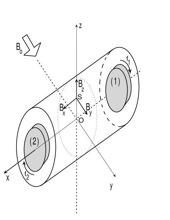
Figure 1: Geometry of the experimental set-up. The flow is generated by rotating only one disk either at position (1) or (2). The magnetic field is measured at position $S$.

We have measured the induced magnetic field $\vec{B}$ generated by a turbulent von Kármán swirling flow of liquid sodium submitted to a transverse external magnetic field $\vec{B}_{0}$ (see Fig. 1). The sodium flow is operated in a loop that has been described elsewhere together with the details of the experimental set-up vks01 . The flow is driven by rotating one of the two disks of radius $R$ located at position (1) or (2) in a cylindrical vessel, $40$ cm in inner diameter and $40$ cm in length. In most experiments presented here, we use a disk of radius $R=150$ mm, fitted with 8 straight blades of height $h=10$ mm driven at a rotation frequency up to $f=30$ Hz. Four baffles, $20$ mm in height, have been mounted on the cylindrical vessel inner wall, parallel to its axis. A turbulent swirling flow with an integral Reynolds number, $Re=2\pi R^{2}f/\nu$, up to $3\times 10^{6}$ is driven by the rotating disk. The mean flow has the following characteristics: the fluid is ejected radially outward by the disk; this drives an axial flow toward the disk along its axis and a recirculation in the opposite direction along the cylinder lateral boundary. The baffles inhibit the azimuthal velocity of the recirculating flow and thus prevent a global rotation of the fluid. In some experiments, we have used a disk of radius $R=190$ mm, fitted with 16 curved blades of height $h=40$ mm, with or without the lateral baffles in order to observe the effect of a stronger azimuthal flow.

Two Helmholtz coils generate a magnetic field $\vec{B}_{0}$, perpendicular to the cylinder axis (see Fig. 1). The three components of the field induced by the flow are measured with a 3D Hall probe, located $180$ mm away from the disk in the plane perpendicular to $\vec{B}_{0}$ and containing the rotation axis. The probe distance from the rotation axis is adjustable ($z=42,100,150$ mm).

The equations governing the magnetic field $\vec{B}_{0}+\vec{B}(\vec{r},t)$, where $\vec{B}(\vec{r},t)$ is the magnetic field generated by the flow in the presence of the applied field $\vec{B}_{0}$, are in the MHD approximation,

$$\vec{\nabla}\cdot\vec{B}=0,$$ (1)

$$\frac{\partial{\vec{B}}}{\partial{t}}=\vec{\nabla}\times\left(\vec{V}\times(\vec{B}+\vec{B}_{0})\right)+{1\over\mu_{0}\sigma}\Delta\vec{B},$$ (2)

where $\vec{V}(\vec{r},t)$ is the velocity field, $\mu_{0}$ is the magnetic permeability of vacuum, and $\sigma$ is the fluid electric conductivity.

The reaction of the magnetic field on the flow is characterized by the ratio of the Lorentz force to the characteristic pressure forces driving the flow. This is measured by the interaction parameter, $N=B_{0}^{2}/\rho\mu_{0}U^{2}$, where $\rho$ is the fluid density and $U$ is the characteristic velocity of the solid boundaries driving the fluid motion. The maximum field amplitude being $B_{0}=12$ G, $N$ is in the range $10^{-5}-10^{-3}$, thus the effect of the magnetic field on the flow is negligible in our experiments. This has been checked directly by measuring the induced magnetic field as a function of the applied one at a constant driving of the flow. We calculate the mean induced field $\langle\vec{B}\rangle$ where $\langle\cdot\rangle$ stands for average in time, as well as its $rms$ fluctuations in time, $\vec{B}_{rms}$. Both vary linearly with $B_{0}$, thus showing that the modification of the velocity field $\vec{V}$ in Eq. (2) can be neglected when $B_{0}$ is increased vks01 . Thus, the only relevant dimensionless parameter of our experiments is the magnetic Reynolds number, $R_{m}=\mu_{0}\sigma RU=2\pi\mu_{0}\sigma R^{2}f$, which is proportional to the rotation frequency $f$ and has been varied up to 40 for radius of the disks $R=150$ mm (respectively $55$ for $R=190$ mm).

The three components of the mean magnetic field $\vec{B}_{0}+\langle\vec{B}(\vec{r})\rangle$, at $z=100$ mm above the rotation axis, are displayed in Fig. 2 as a function of the rotation frequency. We observe that when the rotation of the disk is reversed, $f\rightarrow-f$, we approximately get $\left(\langle B_{x}\rangle,\langle B_{y}\rangle,\langle B_{z}\rangle\right)\rightarrow\left(-\langle B_{x}\rangle,\langle B_{y}\rangle,-\langle B_{z}\rangle\right)$. When disk (2) is rotated instead of (1) but keeping $f$ unchanged, we get $\left(\langle B_{x}\rangle,\langle B_{y}\rangle,\langle B_{z}\rangle\right)\rightarrow\left(-\langle B_{x}\rangle,\langle B_{y}\rangle,\langle B_{z}\rangle\right)$ (note that the measurements of $\vec{B}$ are performed in the mid-plane between the two disks). Assuming that the swirling flow has not broken the symmetries of the driving configuration, the above transformations of the field components can be understood using the following symmetry transformations:

- (i) the symmetry with respect to the vertical plane perpendicular to $\vec{B}_{0}$, $x0z$, shows that if the disk is rotated in the opposite way, $f\rightarrow-f$, we get $\left(\langle B_{x}\rangle,\langle B_{y}\rangle,\langle B_{z}\rangle\right)\rightarrow\left(-\langle B_{x}\rangle,\langle B_{y}\rangle,-\langle B_{z}\rangle\right)$ ($\vec{B}$ is a pseudovector).

- (ii) The symmetry with respect to the vertical plane parallel to $\vec{B}_{0}$, $y0z$, followed by the transformation $\vec{B}_{0}\rightarrow-\vec{B}_{0}$, shows that when we rotate disk (2) instead of disk (1) without changing the sign of $f$, we get $\left(\langle B_{x}\rangle,\langle B_{y}\rangle,\langle B_{z}\rangle\right)\rightarrow\left(-\langle B_{x}\rangle,\langle B_{y}\rangle,\langle B_{z}\rangle\right)$.

The induced field component $\langle B_{y}\rangle$ is opposed to $\vec{B}_{0}$ and increases in amplitude, thus the total field along $\vec{B}_{0}$ decreases as $R_{m}$ is increased. This expulsion of a transverse magnetic field from eddies is well documented, both theoretically par66 ; wei66 and experimentally odi00 . The expulsion is stronger close to the axis of the cylinder ($z=42$ mm). On the contrary, closer to the cylinder lateral boundary ($z=150$ mm), the field increases with $R_{m}$. Thus, the field is expelled from the core of the swirling flow and concentrates at its periphery.

The components of the field induced perpendicular to $\vec{B}_{0}$ both increase in amplitude from zero, reach a maximum and then saturate when $R_{m}$ is increased further. As shown in Fig. 3, these two components do not scale in the same way at small rotation frequency, i.e. at small $R_{m}$. The amplitude of the vertical component $\langle B_{z}\rangle$ increases linearly whereas the axial component $\langle B_{x}\rangle$ increases quadratically with $R_{m}$. Indeed, at the location of the measurements, we observe $\langle B_{x}\rangle\propto\langle B_{z}\rangle^{2}$ and $\langle B_{y}\rangle\propto\langle B_{z}\rangle^{2}$, roughly up to $f=10$ Hz (see Fig. 3).

Writing $\vec{B}(\vec{r},t)=\langle\vec{B}(\vec{r})\rangle+\vec{b}(\vec{r},t)$, and similarly for $\vec{V}$, we get from Eq. (2) for the mean induced field

$$-{1\over\mu_{0}\sigma}\Delta\vec{\langle B\rangle}=\vec{\nabla}\times\left(\vec{\langle V\rangle}\times\vec{B}_{0}+\vec{\langle V\rangle}\times\vec{\langle B\rangle}+\langle\vec{v}\times\vec{b}\rangle\right).$$ (3)

When the magnetic Reynolds number is small, the first source term on the right hand side of Eq. (3) is the dominant term and we get for each component of the mean induced field $\langle B_{i}\rangle\propto R_{m}B_{0}$. However, both the expulsion of a transverse field from a rotating eddy and the $\alpha$-effect, i.e. the generation of a current parallel to an applied field by a cyclonic eddy, cannot be described at this level and involve the nonlinear source terms of Eq. (3).

Indeed, keeping only the contribution of the first term on the right hand side of equation (3) gives for $\langle B_{x}\rangle$

$$-{1\over\mu_{0}\sigma}\Delta{\langle B_{x}\rangle}={B}_{0}\frac{\partial\langle V_{x}\rangle}{\partial y}\,.$$ (4)

The source term being antisymmetric with respect to the vertical plane $x0z$, we have for the linear response $\langle B_{x}(x,y=0,z)\rangle=0$.

The generation of $B_{x}$ is the consequence of the $\alpha$-effect, i.e. of the generation of a current parallel to $\vec{B}_{0}$. Indeed, at leading order in $R_{m}$, $\langle B_{x}\rangle$ increases like $R_{m}^{2}$ and its sign with respect to the sign of $B_{0}$ is determined by the flow helicity, $h=\overline{\vec{V}\cdot(\vec{\nabla}\times\vec{V})}$ where the overbar stands for the spatial average. One can easily check that $\langle B_{x}\rangle$ changes sign under any symmetry with respect to a plane containing the rotation axis, just as does the pseudoscalar $h$.

For fixed $R_{m}$, $\langle B_{x}\rangle$ increases with the distance to the cylinder axis in the range $42<z<150$ mm. We can show that it should vanish for $z=0$: indeed, the rotation of angle $\pi$ around the $x$-axis followed by the transformation $\vec{B}_{0}\rightarrow-\vec{B}_{0}$ which implies $\vec{B}\rightarrow-\vec{B}$, gives $\langle B_{x}(x,0,z)\rangle=-\langle B_{x}(x,0,-z)\rangle$.

When $R_{m}$ is increased $\langle B_{x}\rangle$ seems to saturate for $z=100$ mm (see Fig.2). Closer to the rotation axis ($z=42$ mm), it reaches a maximum and then decreases roughly to zero when $f$ is increased up to $30$ Hz. This is due to the expulsion of the applied magnetic field $\vec{B}_{0}$ from the core of the swirling flow. Indeed, when the baffles are removed from the cylindrical vessel inner wall, global rotation of the flow is no longer inhibited, and $\langle B_{x}\rangle$ measured $100$ mm away from the rotation axis, decreases to zero at large $R_{m}$ (see Fig. 4 and compare with Fig. 2 where $\langle B_{x}\rangle$ stays finite at large $R_{m}$). Consequently, we observe that the $\alpha$-effect decays when $R_{m}$ is too large, or more precisely when the magnetic Reynolds number corresponding to the azimuthal flow is too large, because of the transverse field expulsion from the cyclonic eddy. A similar effect has been recently computed by Rädler et al. in the case of the Roberts flow rad97 . They have shown by computing terms higher than the second order in $R_{m}$, that the $\alpha$-effect reaches a maximum and then tends to zero when $R_{m}$ is increased further (compare their Fig. 3 with our Fig. 4). Our measurements are the first experimental demonstration that for large $R_{m}$ the $\alpha$-effect can vanish due to the geometry of the flow (i.e. when the amplitude of the azimuthal component of the swirling flow is too large compared to the axial component).

Using dimensional analysis, we can write

$$\langle B_{x}(\vec{r})\rangle=B_{0}\,{\cal F}(\vec{r},R_{m},P_{m},N),$$ (5)

where $P_{m}=\mu_{0}\sigma\nu$ is the magnetic Prandtl number ($\nu$ is the kinematic viscosity). As said above, for $B_{0}$ small enough, ${\cal F}$ does not depend on the interaction parameter $N$. The only previous experimental study of the $\alpha$-effect ste68 considers a constrained flow configuration in a range of $B_{0}$ for which a dependence on $N$ but no dependence on $R_{m}$ have been found. The dependence on $N$ can give insights on the nonlinear saturation mechanism of a dynamo generated via the $\alpha$-effect. On the contrary, the dependence on $R_{m}$ determines the dependence of the linear growth rate of a dynamo generated via the $\alpha$-effect. The decay of the $\alpha$-effect for large $R_{m}$ reported here, gives a possible mechanism for a “slow dynamo”, i.e. a dynamo with a growth rate that decreases at large $R_{m}$. Finally, the dependence on $P_{m}$, or equivalently on the Reynolds number of the flow, cannot be determined from our measurements. In other words, we do not know the contribution of the turbulent fluctuations to the measured $\alpha$-effect, i.e. the relative contribution of the two nonlinear source terms $\vec{\nabla}\times\left(\vec{\langle V\rangle}\times\vec{\langle B\rangle}\right)$ and $\vec{\nabla}\times\left(\langle\vec{v}\times\vec{b}\rangle\right)$ in equation (3). Both the velocity field, measured in water vks01 , and the magnetic field display large fluctuations (roughly $20\%$), but we cannot evaluate $\langle\vec{v}\times\vec{b}\rangle$. It would be of great interest to develop a device for simultaneous measurements of magnetic and velocity fields, or to perform experiments with different liquid metals in order to quantify the effect of $P_{m}$. Indeed, the effect of $P_{m}$ on the induced fields can give insights in the problem of the dependence of an $\alpha$-dynamo threshold, $R_{m}^{c}$, on $P_{m}$ or equivalently on the Reynolds number of the flow. The behavior of $R_{m}^{c}$ in the limit of large Reynolds number is an open problem of kinematic dynamo theory and is of prime experimental and theoretical interest.

We gratefully acknowledge the assistance of J.-B. Luciani and M. Moulin and the financial support of the french institutions: Direction des Sciences de la Matière and Direction de l’Energie Nucléaire of CEA, Ministère de la Recherche and Centre National de Recherche Scientifique. J. Burguete was supported by post-doctoral grant No. PB98-0208 from ministerio de Educacion y Ciencias (Spain) while at CEA-Saclay.

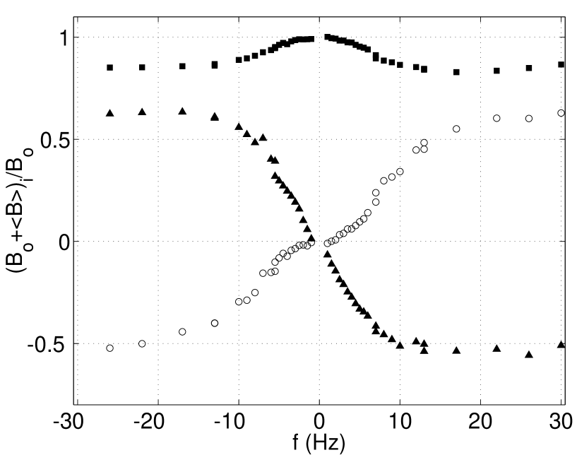
Figure 2: Components of the total mean magnetic field as a function of the rotation frequency of disk (2). The disk radius is $R=150$ mm with straight blades. Four baffles are mounted on the inner wall of the cylindrical vessel. The magnetic field is measured at $z=100$ mm. (($o$) $=\frac{\langle B_{x}\rangle}{B_{o}}$, ($\blacksquare$)$=\frac{B_{o}+\langle B_{y}\rangle}{B_{o}}$,($\blacktriangle$)$=\frac{\langle B_{z}\rangle}{B_{o}}$)

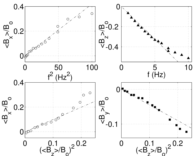
Figure 3: (a-b): Axial and vertical mean components of the induced magnetic field as a function of the rotation frequency. (c-d): Axial and transverse mean components of the induced magnetic field as a function of the square of the vertical one, for $f<10\,Hz$. Same experimental configuration as in Fig. 2.

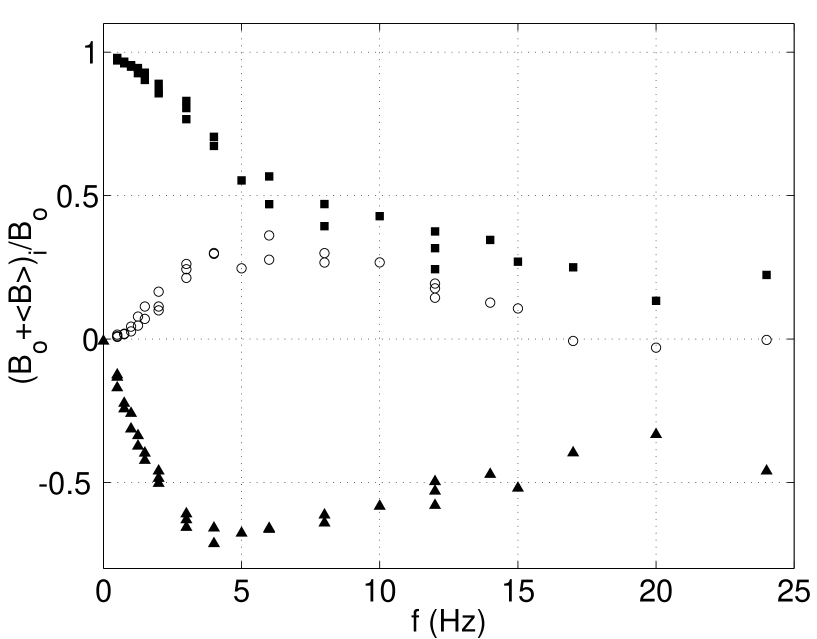
Figure 4: Components of the total mean magnetic field as a function of the rotation frequency of the disk (2). The disk radius is $R=190$ mm with curved blades. There are no baffles on the inner wall of the cylindrical vessel. The magnetic field is measured at $z=100$ mm. (($o$) $=\frac{\langle B_{x}\rangle}{B_{o}}$, ($\blacksquare$)$=\frac{B_{o}+\langle B_{y}\rangle}{B_{o}}$,($\blacktriangle$)$=\frac{\langle B_{z}\rangle}{B_{o}}$)

References

- (1) E. N. Parker, Astrophysical J. 122, 293 (1955).
- (2) F. Krause and K.-H. Rädler, Mean field magnetohydrodynamics and dynamo theory, Pergamon Press (New-York, 1980).
- (3) H. K. Moffatt, Magnetic field generation in electrically conducting fluids, Cambridge University Press (Cambridge, 1978).
- (4) P. H. Roberts, in Lectures on solar and planetary dynamos , chap. 1, M. R. E. Proctor and A. D. Gilbert eds., Cambridge University Press (Cambridge, 1994).
- (5) R. Stieglitz and U. Müller, Phys. Fluids 13, 561 (2001).
- (6) A. Gailitis, O. Lielausis, E. Platacis, S. Dement’ev, A. Cifersons, G. Gerbeth, T. Gundrum, F. Stefani, M. Christen and G. Will, Phys. Rev. Lett. 86, 3024 (2001).
- (7) P. H. Roberts, in Irreversible phenomena and dynamical systems analysis in geosciences, 73-133, C. Nicolis and G. Nicolis eds., Reidel (1987).
- (8) M. Steenbeck, I. M. Kirko, A. Gailitis, A. P. Klyavinya, F. Krause, I. Ya. Laumanis and O. A. Lielausis, Sov. Phys. Dok. 13, 443 (1968).
- (9) see for instance, Dynamo and dynamics, a mathematical challenge, P. Chossat et al. (eds.), L. Marié et al. “MHD in von Kármán swirling flows”, pp. 35-50, R. O’Connell et al., “On the possibility of an homogeneous MHD dynamo in the laboratory”, pp. 59-66, W. L. Shew et al. “Hunting for dynamos: height different liquid sodium flows”, pp. 83-92, Kluwer Academic Publishers (2001).
- (10) M. Bourgoin et al., “MHD measurements in the von Kármán sodium experiment”, submitted to Phys. Fluids (2001).
- (11) R. L. Parker, Proc. Roy. Soc. A 291, 60 (1966).
- (12) N. O. Weiss, Proc. Roy. Soc. A 293, 310 (1966).
- (13) P. Odier, J.-F. Pinton and S. Fauve, Eur. Phys. J. B 16, 373 (2000).
- (14) K.-H. Rädler, E. Apstein and M. Schüler, “The -effect in the Karlsruhe dynamo experiment” in Transfer phenomena in magnetohydrodynamic and electroconducting flows, 1, 9-14 (1997).