Molecular gyroscopes and biological effects of weak ELF magnetic fields

Abstract

Extremely-low-frequency magnetic fields are known to affect biological systems. In many cases, biological effects display ‘windows’ in biologically effective parameters of the magnetic fields: most dramatic is the fact that relatively intense magnetic fields sometimes do not cause appreciable effect, while smaller fields of the order of 10–100 $\mu$T do. Linear resonant physical processes do not explain frequency windows in this case. Amplitude window phenomena suggest a nonlinear physical mechanism. Such a nonlinear mechanism has been proposed recently to explain those ‘windows’. It considers quantum-interference effects on protein-bound substrate ions. Magnetic fields cause an interference of ion quantum states and change the probability of ion-protein dissociation. This ion-interference mechanism predicts specific magnetic-field frequency and amplitude windows within which biological effects occur. It agrees with a lot of experiments. However, according to the mechanism, the lifetime $\Gamma^{-1}$ of ion quantum states within a protein cavity should be of unrealistic value, more than 0.01 s for frequency band 10–100 Hz. In this paper, a biophysical mechanism has been proposed that (i) retains the attractive features of the ion interference mechanism, i.e., predicts physical characteristics that might be experimentally examined and (ii) uses the principles of gyroscopic motion and removes the necessity to postulate large lifetimes. The mechanism considers dynamics of the density matrix of the molecular groups, which are attached to the walls of protein cavities by two covalent bonds, i.e., molecular gyroscopes. Numerical computations have shown almost free rotations of the molecular gyros. The relaxation time due to van der Waals forces was about 0.01 s for the cavity size of 28 angströms.

I Introduction

Weak static and extremely-low-frequency (ELF) magnetic fields (MFs) can affect living things: cells, tissues, physiological systems, and whole organisms Blank (1995); Goodman et al. (1995); Bersani (1999). In many cases biological effects of weak MF feature resonance-like multipeak behavior. Multipeak responses or magnetobiological spectra may appear with varying the frequency or amplitude of AC MF Adey (1993) and the magnitude of DC MF Belyaev et al. (1994). Usually, the term ‘windows’ is used for the peaks of the spectra.

Amplitude ‘windows’, see Fig. 1, specify nonlinearity of the transduction mechanisms involved in magnetobiological effects. This is confirmed more by the fact that magnetic noise simultaneously superimposed on a regular magnetic signal suppresses biological effect of that signal Mullins et al. (1993); Lin and Goodman (1995); Raskmark and Kwee (1996); Litovitz et al. (1997).

A nonlinear mechanism based on quantum interference has been developed in Binhi (1997) to explain unusual ELF MF frequency and amplitude dependencies of magnetobiological effects (MBEs). The mechanism elaborates the interference of ions bound within proteins. According to this mechanism, superposition of the ion states forms a non-uniform pattern of the probability density of ion. This pattern consists of a row of more or less dense segments occurring due to the interference between quantum states of ions in a protein binding cavity. In a DC MF the pattern rotates with the cyclotron frequency. Exposure to a time-varying MF of specific parameters retards the rotation of the pattern and facilitates escape of the ion from the cavity. This escape might influence equilibrium of biochemical reactions to ultimately result in a biological effect.

Biologically effective parameters of AC-DC magnetic fields depend on the charge-to-mass ratio of the ion in question. The closed formula is derived for ‘magnetic’ part P of ion-protein dissociation probability. Predictions based on this formula reveal good agreement with experimental results involving calcium, magnesium, potassium, hydrogen and other ions of as molecular targets for MF. The theory describes multipeak frequency and amplitude spectra of MBEs involving ions of Ca²⁺, Mg²⁺, and H⁺ as molecular targets for AC-DC MFs Binhi (1997).

The interference mechanism is surprisingly effective in retrospectively predicting results of existing experiments conducted under the following defined MF conditions: parallel AC-DC and pulsed MFs Binhi (1997, 1998), ‘null’ and static MFs Binhi et al. (2001), and various MFs with a slow rotation of a biological system Binhi (2000). As an example, Fig. 1 demonstrates the comparison of experimental data, in parallel AC-DC MFs, on MBEs involving fixed and rotating proteins, and calculated curve (dash line).

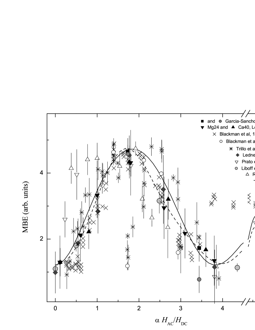
Figure 1: Experimental evidence Liboff et al. (1987); Ross (1990); Blackman et al. (1994); Garcia-Sancho et al. (1994); Blackman et al. (1995); Prato et al. (1995); Lednev et al. (1996a, b); Trillo et al. (1996); Blackman et al. (1999) for MBEs in a uniaxial MF (Ross (1990) noted a weak perpendicular component of a DC MF). Theoretical amplitude spectra: a dash line was derived for fixed ion-protein complexes (factor $\alpha=1$ was not shown) and also for rotating ion-protein complexes, see details in Binhi (2000). Solid line represents the function (18) derived for gyro interference.

The good consistency between theoretical calculations and many experiments indicates that what underlies magnetobiological effects is most likely an interference phenomenon.

According to the interference mechanism, the relation should be valid $\Gamma^{-1}\Omega_{\rm c}\gtrsim 1$, where $\Gamma^{-1}$ is the lifetime of ion quantum states within a bound cavity and $\Omega_{\rm c}$ is a cyclotron frequency of an ion in the geomagnetic field, usually 10–100 Hz. The postulate therefore has to be made that ion quantum states, more exactly their angular modes, live more than 0.01 s within the cavity. However it is in contradiction with our common knowledge that such states might live only $10^{-12}$–$10^{-10}$ s because of the thermalizing interaction of ion with cavity walls. On the other hand, the weak AC MF, $\hbar\Omega_{\rm c}\ll k_{{}_{\rm B}}T$, is commonly believed to be unable to contribute into thermally driven (bio)chemical reactions (so-called kT-problem).

To overcome the problem, we note that there is a specific mechanism that provides relatively large lifetime of the angular modes. Consider a dipole molecular group that are attached within the cavity to its walls in two points, i.e. by two covalent bonds, thus forming a group that may rotate inside the cavity without contact with walls. Such a construction is referred to as gyroscope. In the case, it is a molecular gyroscope. Of importance is the fact that thermal oscillations of that covalent bonds, or gyroscope’s supports, make only zero torque about the axis of rotation. This leads to relatively slow thermalization of a gyroscopic degree of freedom. Relaxation is mainly due to van der Waals interaction with thermalizing walls. As far as the interaction potential, the Lennard–Jones potential, decreases as $r^{-6}$ and walls’ inner surface grows as $r^{2}$, the overall van der Waals contribution varies approximately as $r^{-4}$. That is, relaxation quickly diminishes with the cavity size to grow. Computations show almost free rotations (thermalization time 0.01 s) of a molecular gyro within the cavity of 28 angströms size. This is enough for the ion interference mechanism to display itself. Probably, such roomy cavities are formed by ensembles of a few protein globules, between them, or within some enzymes that unfold DNA double-helix.

II Molecular gyroscope

A long lifetime of angular modes is the sole serious idealization underlying the mechanism of ion interference. This idealization would be hard to substantiate with the ion-in-protein-capsule model. One would have to assume that the ion forms bound states of the polaron type with capsule walls. In turn, justification of a large lifetime of polaron angular modes would require new idealizations. A ‘vicious circle’ occurs which one could not leave without having to substantially change the model itself. Thus, despite the obvious advantages of the ion-in-capsule model, namely, simplicity and a high forecasting skill, we have to recognize its limitations and seek for other solutions.

One of them hinges on the use of conservation laws in the dynamics of rotating solids. Rotation of a solid is described by the equation

$$\frac{d{\bf L}}{dt}={\bf K},$$ (1)

where $\bf L$ is the angular momentum, $\bf K$ is the sum of torques acting on the solid. Consider for simplicity a symmetric gyro rotating around one of its main axes of inertia with a force $\bf F$ acting on its point of support, as shown in Fig. 2. The moment of this force about the shown axis is obviously zero. From equation (1) we have

$${\bf L}={\bf L}_{0}+d{\bf L},~{}~{}~{}d{\bf L}={\bf K}\,dt={\bf r}\times{\bf F}dt.$$

Since ${\bf K}\perp{\bf F}$, then $d{\bf L}\perp{\bf F}$, i.e., the force caused an orthogonal displacement of the axis of rotation. Also, the vector $\bf r$ is directed along the axis of rotation, therefore the vector $d{\bf L}$ is also orthogonal with ${\bf L}_{0}$.

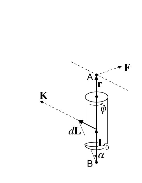
Figure 2: Forces, moments of forces, and angular momenta in rotation of a gyro.

Thus, a continuously acting force $\bf F$ causes a forced precession of the gyro about the direction $\bf F$ with an angular velocity defined by the angle through which the gyro axis of rotation deviates per unit time, viz.,

$$\Omega_{\rm precession}=\frac{d{\bf L}/{\bf L}_{0}}{dt}=\frac{K}{L_{0}}=\frac{rF}{L_{0}}.$$

The length of vector $\bf r$ is defined by the gyro locking conditions. If point B is fixed, then the origin of $\bf r$ coincides with B. If point B is free, then the origin of $\bf r$ is on line AB and depends on the gyro parameters. For estimation, it is important that $r$ has the order of magnitude of gyro length.

Let the gyro be a model of a rigid molecule free to move and constrained by the thermal oscillations of one of the point of support (e.g. A) alone. We estimate the mean gyro axis deviation angle for a random force $\bf F$ causing chaotic oscillations of its point of support. It should be noted that the gyro gravity energy $\sim MgR$ is many orders of magnitude below its kinetic energy $\sim L^{2}/2I$ and the effects of gravity may be neglected. In the last formulas, $M,R$, and $I$ are the gyro mass, size, and moment of inertia, and $g$ is the acceleration due to gravity.

The energy of natural gyro rotation is $\varepsilon_{0}=L_{0}^{2}/2I$. The gyro energy including chaotic rotations is $\varepsilon_{0}+k_{{}_{\rm B}}T$. On the other hand, the mean energy with allowance for orthogonality of ${\bf L}_{0}$ and $d{\bf L}$ is

$$\langle\frac{1}{2I}({\bf L}_{0}+d{\bf L})^{2}\rangle=\frac{1}{2I}\left\{L_{0}^{2}+2\langle{\bf L}_{0}d{\bf L}\rangle+\langle d^{2}{\bf L}\rangle\right\}$$

$$=\varepsilon_{0}+\frac{\langle d^{2}L\rangle}{2I},$$ (2)

where brackets mean averaging over the ensemble. Then ${\langle d^{2}L\rangle}/{2I}\sim k_{{}_{\rm B}}T$. Denoting the average deviation angle by $\alpha=\sqrt{\langle d^{2}L\rangle}/L_{0}$ yields $\alpha^{2}\sim 2Ik_{{}_{\rm B}}T/L_{0}^{2}$. The smaller $L_{0}$ the larger the random deviations of a molecule caused by thermal perturbations of its support. Such a support is the covalent bond with the body of protein molecule. Low bound estimates of $L_{0}$ follow from the Heisenberg uncertainty principle which, for a complementary pair of noncommuting operators of angular variable $\varphi$ and angular momentum ${\mathcal{L}}\sim d\,/d\varphi$, can be written as:

$$\triangle L\,\triangle\varphi\sim\hbar/2.$$

Since $\triangle\varphi\sim\pi$, then $\triangle L\sim\hbar/2\pi$; thus the angular momentum cannot be smaller than its uncertainty, i.e., $L_{0}\sim\hbar/2\pi$. Finally, we have

$$\alpha^{2}\sim 8\pi^{2}\frac{Ik_{{}_{\rm B}}T}{\hbar^{2}}.$$

As can be seen deviations increase with the size of molecule; however, even for small molecules, the estimate of deviation is unrealistically large. It implies that, in lower rotation states, molecules will ‘lay aside’ in response to perturbation of their support and, consequently, the angular momentum will not be conserved. It should be noted that we are interested only in angular states with small quantum numbers. Otherwise the interference patterns to be discussed below become fine grained and are unlikely to be reflected in measured properties.

Thus, in order to be immune to thermal displacements of supports, the gyro has to have its second support also fixed in the protein matrix. The configuration of a rotating solid with supports fixed in the rim is one of the types of a gyroscope, i.e., a device to measure angular displacements and velocities. What we consider is essentially a molecular gyro: a relatively large molecular group is placed in a protein cavity and its two edges form covalent bonds (supports) with the cavity walls. It is important to note that thermal oscillations of the supports produce only zero moments of forces about the natural group rotation axis. Therefore, the gyroscopic degree of freedom $\varphi$ is not thermalized by the supports’ oscillations. This does not imply that the energy of the gyro does not dissipate. Radiation damping or Lorentz friction force is neglected, because of its infinitesimal value. Below we examine at first the interference of the molecular gyro and then the damping due to wan der Waals forces.

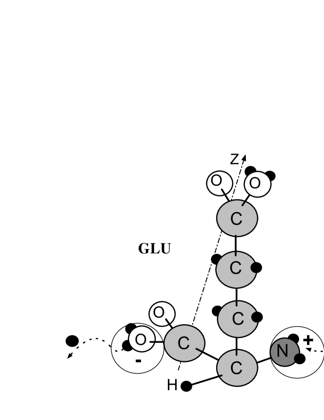
Figure 3: An amino glutaric acid molecule with potentially ionizing groups. The $z$ axis is the main axis of inertia. Rotation of charges distributed over the molecule in a magnetic field leads to interference of its quantum angular states.

III Interference of the molecular gyroscope

Rotations of large molecules is much slower a process than electron and oscillatory processes. Therefore, we think of the rotating molecular group as a rigid system of charged point masses — atoms and molecules with partially polarized chemical bonds. To illustrate, we point to molecules of amino acids which could be built into rather spacious protein cavities forming chemical bonds at extreme ends of the molecule, thus forming a molecular gyroscope. Amino acids are links of polymeric protein macromolecules and also occur in a bioplasm as free monomers. The general formula of amino acids is well known:

$${\rm R}$$

$$|$$

$$~{}~{}~{}~{}~{}{\rm H}_{2}{\rm N}^{+}-{\rm C}{\rm H}-{\rm C}{\rm O}{\rm H}{\rm O}^{-} ~{},$$

where R is a radical which differs one molecule from another. Polarities of the groups are shown in a water solution. By way of example, the radical of amino glutaric acid consists of three links $-{\rm C}{\rm H}_{2}-{\rm C}{\rm H}_{2}-{\rm C}{\rm O}{\rm O}{\rm H}$, as shown in Fig. 3. Fixed on either side of a cavity, such a molecule, treated as a dynamic unit, has one degree of freedom — a polar angle $\varphi$, which simplifies analysis of its behavior in a magnetic field.

For small velocities, the Lagrange function of one charge particle has the form

$${\sf L}=\frac{Mv^{2}}{2}+\frac{q}{c}{\bf A}{\bf v}-qA_{0},$$ (3)

where $\bf v$ is the particle velocity, and $q$ is a charge. Let the magnetic field ${\bf H}=(0,~{}0,~{}H)$ be directed along the $z$ axis, and the particle be bounded by a holonomic constraint causing its circumferential motion in the $xy$ plane. In spherical coordinates, the constrains can be written in the form

$$r=R=\mbox{\rm const.},~{}~{}~{}\theta={\pi}/2.$$ (4)

We choose the vector potential in the form

$${\bf A}=\left(-\frac{1}{2}Hy,~{}\frac{1}{2}Hx,~{}0\right).$$ (5)

With allowance for constraints (4), the velocity of a particle in spherical coordinates will be $v=R\dot{\varphi}$, and the velocity vector in Cartesian coordinates is

$${\bf v}=\left(-R\dot{\varphi}\sin(\varphi),~{}R\dot{\varphi}\cos(\varphi),~{}0\right).$$ (6)

Substituting this expression in equation (3), we obtain the Lagrange function in spherical coordinates

$${\sf L}=\frac{MR^{2}\dot{\varphi}^{2}}{2}+\frac{qH}{2c}R^{2}\dot{\varphi}-qA_{0}.$$ (7)

Now, the generalized momentum is $l=\partial{\sf L}/\partial\dot{\varphi}$, and the Hamilton function ${\sf H}=l\dot{\varphi}-{\sf L}$ is equal to

$${\sf H}=\frac{1}{2MR^{2}}\left(l-\frac{qH}{2c}R^{2}\right)^{2}+qA_{0}~{}.$$ (8)

In the absence of electromagnetic field ${\sf H}={l^{2}}/{2MR^{2}}$, and it is obvious that $l$ is the angular momentum of the particle. The Hamiltonian operator repeats (8) with the difference that here $l$ is the angular momentum operator ${\mathcal{L}}=-i\hbar{\partial}/{\partial\varphi}$.

Let now a few particles rotate and, in a spherical system of coordinates, the constraints for particle $i$ be

$$r_{i}=\mbox{\rm const.}~{},~{}~{}~{}\theta_{i}=\mbox{\rm const.}$$

Then, for a system of particles in a uniaxial magnetic field, the Lagrange function can be written following the derivation of formula (7) as

$${\sf L}=\frac{I}{2}\dot{\varphi}^{2}+\frac{HQ}{2c}\dot{\varphi}-\sum_{i}q_{i}A_{0}(r_{i},\theta_{i},\varphi_{i})~{},$$ (9)

where

$$I=\sum_{i}M_{i}r_{i}^{2}\sin^{2}(\theta_{i}),~{}~{}~{}Q=\sum_{i}q_{i}r_{i}^{2}\sin^{2}(\theta_{i})$$ (10)

is the moment of inertia, and ‘charge moment of inertia’ of the system about the axis of rotation. As can be seen, the Lagrange function of the system follows from the Lagrange function (7) after formal replacement of $MR^{2}$ with $I$, $qR^{2}$ with $Q$, and $qA_{0}$ with the respective sum. Therefore, the Hamiltonian of the system immediately follows from equation (8) after similar substitutions

$${\mathcal{H}}=\frac{1}{2I}\left({\mathcal{L}}-\frac{QH}{2c}\right)^{2}+\sum_{i}q_{i}A_{0}(r_{i},\theta_{i},\varphi_{i}).$$

We assume further that the electric field is absent, i.e., let $A_{0}=0$:

$${\mathcal{H}}=\frac{1}{2I}\left({\mathcal{L}}-\frac{QH}{2c}\right)^{2}.$$

In addition to ${\mathcal{L}}^{2}/2I$ we find here two more operators. There are certain grounds to neglect the term proportional to squared $H$. From the ratios of coefficients at the terms quadratic and linear in $H$ we obtain $QH/{4c\hbar}\sim 10^{-7}$, where, for estimation purposes, we let $Q\sim eR^{2}$, $R\sim 10^{-7}$ cm, $H\sim 1$ G. Dropping this term we write the Hamiltonian in a convenient form

$${\mathcal{H}}=\frac{{\mathcal{L}}^{2}}{2I}-\omega(t){\mathcal{L}}~{},~{}~{}~{}\omega(t)\equiv\frac{QH}{2Ic}~{}.$$ (11)

The eigenfunctions and energies of the time-independent part of Hamiltonian (11) are

$$|m\rangle=\frac{1}{\sqrt{2\pi}}\exp(im\varphi),~{}~{}m=0,\pm 1,\,...,~{}~{}~{}~{}\varepsilon_{m}=\frac{\hbar^{2}}{2I}m^{2}~{}.$$

We now consider the ensemble of gyros that features a density operator $\sigma$ obeying the Liouville equation

$$i\hbar\dot{\sigma}={\cal H}\sigma-\sigma{\cal H}~{},~{}~{}~{}\sigma=\sum_{\alpha}w_{(\alpha)}\sigma^{(\alpha)}~{}.$$ (12)

Some physical quantities, like the intensity of a spontaneous emission or the radiation reemitted by an ensemble, are known to linearly depend on the density matrix of the ensemble

$$\sigma_{mm^{\prime}}=\sum_{\alpha}w_{(\alpha)}\sigma^{(\alpha)}_{mm^{\prime}}~{}.$$

The probability of biochemical reaction that we examine here is not a quantity of that sort. The reaction probability does not directly depend on the density matrix of the ensemble. It is rather the probability of the reaction of a gyro averaged over that ensemble. Therefore, at first we will find the density matrix $\sigma^{(\alpha)}_{mm^{\prime}}$ of the $\alpha$th gyro, then the reaction probability of that gyro that non-linearly depends on $\sigma^{(\alpha)}_{mm^{\prime}}$, and at last we will average the result over the gyro ensemble.

Let the ensemble consist of gyros that appear with a constant rate at random moments of time. We assume the new gyros appear in a quantum state that is a superposition of the states close to the ground one, i.e.,

$$\sigma^{(\alpha)}_{mm^{\prime}}(0)=\left\{\begin{array}[]{rl}{\rm const}~{},&~{}~{}m,m^{\prime}\sim 1\\ 0~{},&~{}~{}m,m^{\prime}\nsim 1\end{array}\right.~{}.$$

In the process of thermalization, the levels turn out to be populated with the energies up to $\varepsilon_{m}\sim k_{{}_{\rm B}}T$, i.e., with numbers up to $m\sim\frac{1}{\hbar}\sqrt{Ik_{{}_{\rm B}}T}\sim 10^{3}$ for gyros with the inertia moments of the order of $I\sim 10^{35}$ g$\cdot$cm². However, we are interested in the dynamics of the lowest states, that only could result in observable effects.

In the representation of the eigenfunctions of ${\cal H}_{0}$ the density matrix equation may be written from (11) and (12) as follows

$$\dot{\sigma}_{mm^{\prime}}=-(\Gamma_{mm^{\prime}}+i\omega_{mm^{\prime}})\sigma_{mm^{\prime}}-\frac{i}{\hbar}\sum_{l}({\cal V}_{ml}\sigma_{lm^{\prime}}-\sigma_{ml}{\cal V}_{lm^{\prime}})~{},$$ (13)

where

$$\omega_{mm^{\prime}}=\frac{\hbar}{2I}(m^{2}-m^{\prime 2})~{},~{}~{}~{}{\cal V}_{ml}=-\hbar\omega(t)m\delta_{ml}~{}.$$

Phenomenological relaxation of the density matrix elements is taken into account, through the damping constants $\Gamma_{mm^{\prime}}$. Because of the relaxation the elements $\sigma_{mm^{\prime}}$ of the lowest modes decrease while those of upper modes increase. As far as the stationery dynamics of a separate gyro is out of interest, we don’t allow for the pumping upper modes, i.e., population redistribution into the states with large numbers $m$.

Substitution of the above relations in (13) gives rise to the equation

$$\dot{\sigma}=-\Gamma\sigma+i\sigma\left[(m-m^{\prime})\omega(t)-\omega\right]~{},$$

where indices $m,m^{\prime}$ are temporarily omitted for convenience. Along with notation

$$g(t)\equiv-\Gamma+if~{},~{}~{}~{}f\equiv(m-m^{\prime})\omega(t)-\omega$$

the equation takes the straightforward form $\dot{\sigma}=g(t)\sigma$. In the solution of that equation $\sigma=C\exp\left(\int g(t)\,dt\right)$, the constant $C$ follows starting conditions.

Let the MF possesses both DC and AC parts, then

$$\omega(t)=\omega_{\rm g}(1+h^{\prime}\cos\Omega t)~{},~{}~{}~{}\omega_{\rm g}\equiv\frac{QH_{\rm DC}}{2Ic}~{},~{}~{}~{}h^{\prime}\equiv\frac{H_{\rm AC}}{H_{\rm DC}}~{}.$$

Now we separate constant and alternating parts in $g(t)$:

$$g(t)=-x+iz\Omega\cos\Omega t~{},~{}~{}~{}x\equiv\Gamma+i\omega-i(m-m^{\prime})\omega_{\rm g}~{},$$

$$z\equiv(m-m^{\prime})\omega_{\rm g}\frac{h^{\prime}}{\Omega}=(m-m^{\prime})\frac{h^{\prime}}{\Omega^{\prime}}~{},~{}~{}~{}\Omega^{\prime}\equiv\frac{\Omega}{\omega_{\rm g}}~{}.$$

The integral equals

$$\int g(t)\,dt=\int(-x+iz\Omega\cos\Omega t)dt=-xt+iz\sin\Omega t~{},$$

hence

$$\sigma=\sigma(0)e^{\int g(t)\,dt}=\sigma(0)e^{-xt}e^{iz\sin\Omega t}$$

$$=\sigma(0)e^{-xt}\sum_{n}{\rm J}_{n}(z)e^{in\Omega t}~{}.$$

Restoring indeces $m,m^{\prime}$, we arrive at the equation

$$\sigma_{mm^{\prime}}=\sigma_{mm^{\prime}}(0)e^{-[\Gamma_{mm^{\prime}}+i\omega_{mm^{\prime}}-i(m-m^{\prime})\omega_{\rm g}]t}$$

$$\times\sum_{n}{\rm J}_{n}(z_{mm^{\prime}})e^{in\Omega t}~{}.$$

Further, all the damping constants are assumed to equal $\Gamma$. With the notation

$$\beta\equiv\Gamma+i\omega_{mm^{\prime}}-i(m-m^{\prime})\omega_{\rm g}-in\Omega~{},$$

we rewrite the last equation in the form

$$\sigma_{mm^{\prime}}=\sigma_{mm^{\prime}}(0)\sum_{n}{\rm J}_{n}(z_{mm^{\prime}})e^{-\beta t}$$

that will be used later.

Now we consider the probability density of a gyro to take an angular position $\varphi$, which is the only favorable position of the rotating group of the gyro to react with the active site on the wall

$$p(t)=\Psi^{*}(t,\varphi)\Psi(t,\varphi)=\frac{1}{2\pi}\sum_{m}c_{m}^{*}(t)e^{-im\varphi}\sum_{m^{\prime}}c_{m^{\prime}}(t)e^{im^{\prime}\varphi}$$

$$=\frac{1}{2\pi}\sum_{mm^{\prime}}\sigma_{mm^{\prime}}e^{-i(m-m^{\prime})\varphi}~{},$$

that is,

$$p(t)=\frac{1}{2\pi}\sum_{mm^{\prime}n}\sigma_{mm^{\prime}}(0)e^{-i(m-m^{\prime})\varphi}e^{-\beta t}{\rm J}_{n}(z_{mm^{\prime}})~{}.$$

It is expedient to perform a sliding averaging in order to smooth out the relatively fast oscillations: they do not affect the active site that features character time constant $\tau$, i.e.,

$$p_{\tau}(t)=\frac{1}{2\tau}\int_{t-\tau}^{t+\tau}p(t^{\prime})\,dt^{\prime}~{}.$$

Virtually, the factor $\exp(-\beta t)$ should be averaged:

$$\left(e^{-\beta t}\right)_{\tau}=\frac{\sinh(\beta\tau)}{\beta\tau}e^{-\beta t}~{},$$

therefore

$$p_{\tau}(t)=\frac{1}{2\pi}\sum_{mm^{\prime}n}\sigma_{mm^{\prime}}(0)\frac{\sinh(\beta\tau)}{\beta\tau}e^{-i(m-m^{\prime})\varphi}e^{-\beta t}{\rm J}_{n}(z_{mm^{\prime}})~{}.$$ (14)

Then, as in the ion interference model, we assume the reaction probability of a side group of the rotating molecule with the protein active site to be a non-linear function of the probability density (14). In the absence of whatever information on that function, it makes sense to consider quadratic non-linearity, since the linear term makes no contribution to that probability, see details in Binhi (1997). To find the reaction probability we will square (14) and take the average over the gyro ensemble.

In the product $p_{\tau}(t)p_{\tau}(t)$ there are (i) complex conjugate terms, i.e., pairs with indeces $n,m,m^{\prime}$ and $-n,m^{\prime},m$, which apparently do not oscillate, and (ii) fast-oscillating terms that we omit in view of the subsequent averaging. Omitting also immaterial numerical coefficient, we write

$$p_{\tau}^{2}(t)\simeq e^{-2\Gamma t}\sum_{mm^{\prime}n}|\sigma_{mm^{\prime}}(0)|^{2}\left|\frac{\sinh(\beta\tau)}{\beta\tau}\right|^{2}{\rm J}_{n}^{2}(z_{mm^{\prime}})~{}.$$

In this expression, the multiplier

$$S\equiv\sum_{mm^{\prime}n}|\sigma_{mm^{\prime}}(0)|^{2}\left|\frac{\sinh(\beta\tau)}{\beta\tau}\right|^{2}{\rm J}_{n}^{2}(z_{mm^{\prime}})$$

contains the magnetic field dependence.

Let a gyro appear in a moment of time $t^{\prime}$, then the reaction probability at time $t$ equals

$$u(t,t^{\prime})=\left\{\begin{array}[]{rl}Se^{-2\Gamma(t-t^{\prime})}~{},&~{}~{}~{}t\geq t^{\prime}\\ 0~{},&~{}~{}~{}t<t^{\prime}~{}.\end{array}\right.$$

Assuming the moments of time $t^{\prime}$ to be distributed over the gyro ensemble in the interval $(-\theta,\theta)$ with a uniform density $w$ (instead of a discrete distribution for $w_{(\alpha)}$ in (12)), we find the mean probability $\sf P$ by proper integrating over the parameter $t^{\prime}$:

$${\sf P}=\lim_{\theta\rightarrow\infty}w\int_{-\theta}^{\theta}u(t,t^{\prime})\,dt^{\prime}=\frac{wS}{2\Gamma}~{}.$$

To link this value to an observable, e.g., a concentration of the reaction products, we write the kinetic equation for the number $N$ of gyros per unit of tissue volume

$$\dot{N}=w-{\sf P}N$$

that gives $N=w/{\sf P}=2\Gamma/S$ in stationery conditions. Let $S_{0}$ and $N_{0}$ stand for corresponding quantities in the absence of an AC MF, i.e., at $h^{\prime}=0$. We would like to know the relative change $\rho$ of the concentration of the reaction products under the AC MF influence. This is the relative number of gyros entering the reaction, i.e.,

$$\rho\equiv\frac{N_{0}-N}{N_{0}}=1-\frac{S_{0}}{S}~{}.$$ (15)

We now estimate values of $S$ and $\rho$. The following notation will be used:

$$\beta\tau\equiv\eta+i\xi~{},~{}~{}~{}\eta\equiv\Gamma\tau~{},~{}~{}~{}\xi\equiv[\omega_{mm^{\prime}}-(m-m^{\prime})\omega_{\rm g}-n\Omega]\tau~{}.$$

Then the expression for $S$ takes the form

$$S=\sum_{mm^{\prime}n}|\sigma_{mm^{\prime}}(0)|^{2}\frac{\sinh^{2}\eta+\sin^{2}\xi}{\eta^{2}+\xi^{2}}{\rm J}_{n}^{2}\left[(m-m^{\prime})\frac{h^{\prime}}{\Omega^{\prime}}\right].$$ (16)

Since $\eta$ is a constant, the frequency spectrum is defined mainly by the equation $\xi=0$, i.e.,

$$\omega_{mm^{\prime}}-\omega_{\rm g}(m-m^{\prime})-n\Omega=0~{}.$$

For arbitrary small $m$, $m^{\prime}$ frequencies $\omega_{mm^{\prime}}$ fall into the microwave range. The effects of low-frequency MFs are defined by the interference of the levels $m^{\prime}=-m$, when $\omega_{mm^{\prime}}=0$. Then

$$\omega_{\rm g}(m-m^{\prime})+n\Omega=0~{},$$

from which we find

$$\Omega^{\prime}=\frac{2m}{n}~{}.$$ (17)

The series over $n$ in (16) converges quickly, therefore the terms with $n=1$ mainly contribute to the reaction probability. So, at frequencies where the probability gains maxima ($\Omega^{\prime}=2m$) contributions of those terms equal

$$S_{m}\equiv|\sigma_{m,-m}(0)|^{2}\frac{\sinh^{2}(\Gamma\tau)}{\Gamma^{2}\tau^{2}}\,{\rm J}_{1}^{2}(h^{\prime})~{}.$$

Contributions of the terms with $n=2$

$$|\sigma_{m,-m}(0)|^{2}\frac{\sinh^{2}(\Gamma\tau)+\sin^{2}(6m\omega_{\rm g}\tau)}{\tau^{2}(\Gamma^{2}+36m^{2}\omega_{\rm g}^{2})}\,{\rm J}_{2}^{2}(2h^{\prime})~{},$$

obviously, are more than order of value smaller, in the case of $\omega_{\rm g}\gtrsim\Gamma$, i.e., when it makes sense to examine the interference in general. Thus, in order to make approximate assessments we omit the terms with $n>1$. Then, for the same reason, for the ground state $m=0$ only contributions of the terms with $n=0$ are essential. It is those terms that make the contribution independently of an AC MF:

$$S_{0}=|\sigma_{00}(0)|^{2}\frac{\sinh^{2}(\Gamma\tau)}{\Gamma^{2}\tau^{2}}~{}.$$

As well, at a fixed frequency $\Omega^{\prime}=2m^{*}$ only terms with $m=-m^{\prime}=m^{*}$ are essential in their contribution. Now the relative change of the concentration of the reaction products is easy to estimate at the MF frequency, e.g., $\Omega^{\prime}=2m$. Making note of ${\rm J}_{-1}^{2}(h^{\prime})={\rm J}_{1}^{2}(h^{\prime})$ and allowing for $S=S_{0}+S_{m}$ in this case, from (15) we arrive at

$$\rho=1-\left[1+2\frac{\sigma_{-m,m}^{2}(0)}{\sigma_{00}^{2}(0)}{\rm J}_{1}^{2}(h^{\prime})\right]^{-1}~{}.$$

As is seen, the magnitude of the magnetic effect depends on the ratio of the density matrix elements at the initial moment of time just after a gyro appears. For example, if the ground state and the state $m$ (out of Zeeman’s splitting) equipopulated at $t=+0$, then

$$\rho=1-\frac{1}{1+{\rm J}_{1}^{2}(h^{\prime})}~{}.$$ (18)

This function is shown in the Fig. 1, solid line. We conclude that the positions of the maxima of the amplitude spectrum of the magnetic effect do not depend (and the relative magnitude of the effect do) on the distribution of the initial populations of the gyro levels.

The spectrum (17) determines only possible locations of extrema. A real form of the spectrum depends on the initial conditions for the density matrix, i.e., on the populations of levels of different rotational quantum number $m$.

It is instructive to note that the molecule need not have a dipole moment $\sum_{i}q_{i}{\bf r}_{i}$ for the magnetic effect to appear. Rather, it is important that the ‘charge moment of inertia’ $Q$ (10) be other than zero. This can be the case in the absence of dipole moment, e.g. for ionic rather than zwitterionic form of the molecule.

The main properties of the gyro interference are identical with those of the ion interference, namely, (i) multiple peaks in the amplitude and frequency spectra, (ii) dependence of the positions of frequency peaks on the DC MF intensity, and (iii) independence of the positions of amplitude maxima on the AC MF frequency.

We note that the interference of a molecular gyro has some features that differ it from the ion interference. Firstly, the peak frequencies are defined with respect to the gyral frequency $\omega_{\rm g}$ — a rotation equivalent of cyclotron frequency. Peak frequencies depend on the distribution of electric charges over the molecule and may deviate from harmonics and subharmonics of the cyclotron frequency. Secondly, the gyro rotation axis is fixed with respect to the shell, which introduces, in the general case, one more averaging parameter in the model. However, these features are not of principal significance. The specific properties of the interference can always be calculated for any configuration of magnetic and electric fields, for rotation of biological systems and macromolecules involved, etc.

There is the crucial feature of the gyro interference: molecular gyros are relatively immune to thermal shaking and may be effective biophysical targets for external MFs.

As is seen from (16) the absolute magnitude of the magnetic effect, where the latter is maximized by the MF parameters, depends mainly on the value $\eta=\Gamma\tau$, which should be minimized for greater effects. The protein reaction time $\tau$ and the MF frequency $\Omega$ have to fulfill the relation $\Omega\tau\gtrsim 1$ in order to manifest an interference. This and the properties of the function $\sinh^{2}\eta/\eta^{2}$ lead to the condition of observability

$$\Gamma^{-1}\gtrsim\Omega^{-1}\sim 0.01\,\mbox{\rm s}$$ (19)

for the ELF range. The following section examines if the condition is real.

IV Estimating relaxation time from molecular dynamics

Computer simulation of molecular gyro behavior indicates that, for relaxation times of order 0.01 s, the size of cavity should be below 30 Å.

We consider the amino acid residue Phenilalanin, (Phe) C_αC₆H₅, as a gyro and look at the revolution of its benzene ring C₆H₅ about the valence bond C_α—C_β — see Fig. 4. This revolution may be thought of as a rotation in one plane of two rigidly bound point masses $m=26\,m_{\rm p}$ ($m_{\rm p}$ is the mass of proton), spaced by $a=2.42$ Å from one another, about their common center of gravity.

We model the cavity by four heavy particles of mass $M\geq m$ placed in the corners of a square (diagonal $b>a$) centered on the gyro axis, as shown in Fig. 5. We assume that these particles oscillate in the gyro rotation plane $xy$. Each particle moves in the potential well $U(x_{i},y_{i})$, where $x_{i}$, $y_{i}$ is the deviation of particle $i$ from its equilibrium state. The Hamilton function for this system has the form

$${\sf H} = \frac{1}{2}I\dot{\phi}^{2}+\sum_{i=1}^{4}[\frac{1}{2}M(\dot{x}_{i}^{2}+\dot{y}_{i}^{2})+V(\phi,x_{i},y_{i})$$ (20)

$$~{}~{}~{}~{}~{}~{}~{}~{}~{}~{}~{}~{}~{}~{}~{}~{}~{}~{}~{}~{}~{}~{}~{}~{}~{}~{}~{}~{}+U(x_{i},y_{i})],$$

where $I=\frac{1}{2}ma^{2}$ is the gyro moment of inertia, and $\phi$ is its revolution angle.

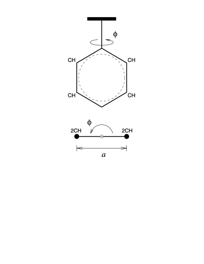
Figure 4: Schematic representation of a molecular gyroscope C_αC₆H₅ reduced to a model of a two-particle rotor of diameter $a$.

We take the potential of interaction of particle $i$ with the gyro as the sum of two Lennard–Jones potentials

$$V(\phi,x_{i},y_{i})=\epsilon\{[(r_{0}/r_{1})^{6}-1]^{2}+[(r_{0}/r_{2})^{6}-1]^{2}\},$$

where $r_{0}$ is the equilibrium arm between a heavy and a light particle, $r_{1}$ is the instantaneous distance of a heavy particle $i$ to the first particle of the gyro, and $r_{2}$ is the distance to the second particle. The interaction of carbon atoms in polymeric macromolecules is commonly described by Lennard–Jones potentials of the form

$$V_{\rm LJ}(r)=4\epsilon_{0}[(\sigma/r)^{12}-(\sigma/r)^{6}]$$

with $\sigma=3.8$ Åand $\epsilon_{0}=0.4937$ kJ/mol Noid et al. (1991); Savin and Manevitch (1998). Recognizing that each particle of the gyro consists of two carbon atoms, we let $\epsilon=1$ kJ/mol $\approx 2\epsilon_{0}$ and $r_{0}=4.5$ Å$\approx 2^{1/6}\sigma$.

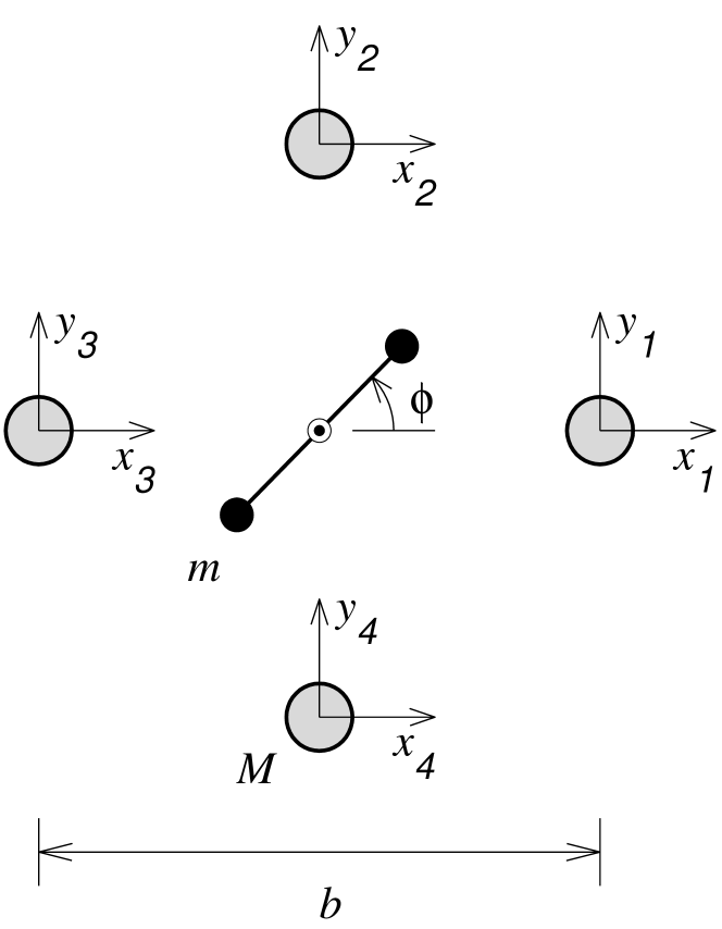
Figure 5: A two-dimensional model of a gyro in a molecular cavity of diameter $b$ formed by four heavy particles of mass $M$.

The carrier potential for each heavy particle will be taken in the form

$$U(x,y)=\frac{1}{2}K\frac{x^{2}+y^{2}}{1-(x^{2}+y^{2})/R_{0}},$$

where $K$ is the rigidity in particle-carrier interaction, and $R_{0}$ is the maximum possible deviation radius of a heavy particle. In a protein macromolecule, the rigidity of atomic displacements is $K=4$ N/m. We consider two maximum displacement values: $R_{0}=1$ Å and $R_{0}=\infty$.

Assuming that heavy particles alone are connected with the thermostat, we obtain the equations of motion in the form

$$I\ddot{\phi} = -\frac{\partial{\sf H}}{\partial\phi},$$

$$M\ddot{x}_{i} = -\frac{\partial{\sf H}}{\partial x_{i}}-\Gamma_{\rm r}M\dot{x}_{i}+\xi_{i},$$ (21)

$$M\ddot{y}_{i} = -\frac{\partial{\sf H}}{\partial y_{i}}-\Gamma_{\rm r}M\dot{y}_{i}+\eta_{i},$$

$$~{}~{}~{}~{}~{}~{}~{}~{}~{}i=1,2,3,4~{},$$

where the system’s Hamilton function is given by equation (20); $\xi_{i}$ and $\eta_{i}$ are random normally distributed forces (white noise) describing the interaction of a heavy particle $i$ with the thermostat, $\Gamma_{\rm r}=1/t_{\rm r}$ is the friction factor, and $t_{\rm r}$ is the particle velocity relaxation time. The correlation functions of random forces are

$$\langle\xi_{i}(t_{1})\xi_{j}(t_{2})\rangle = 2M\Gamma_{\rm r}k_{{}_{\rm B}}T\delta_{ij}\delta(t_{1}-t_{2}),$$

$$\langle\eta_{i}(t_{1})\eta_{j}(t_{2})\rangle = 2M\Gamma_{\rm r}k_{{}_{\rm B}}T\delta_{ij}\delta(t_{1}-t_{2}),$$

$$\langle\xi_{i}(t_{1})\eta_{j}(t_{2})\rangle = 0~{}.$$

Here, $k_{{}_{\rm B}}$ is the Boltzmann constant, and $T$ is the thermostat temperature.

We integrate the equation system (21) by the Runge–Kutta method to the fourth order of accuracy with a constant integration step $\Delta t$. In this computation, the delta function $\delta(t)$ is $0$ for $|t|>\Delta t/2$ and $1/\Delta t$ for $|t|<\Delta t/2$, that is, the integration step corresponds to the correlation time of random force. Therefore, to use a system of Langevin equations, we need that $\Delta t\ll t_{\rm r}$. Let the relaxation time be $t_{\rm r}=0.2$ ps, and the numerical integration step be $\Delta t=0.0025$ ps.

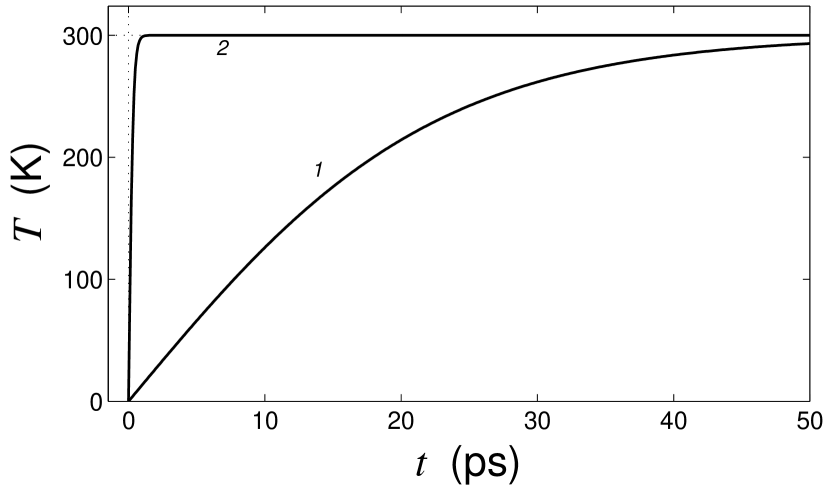
Figure 6: Current mean temperature of the molecular thermostat $T_{1}$ (curve 1) and temperatures of its molecular neighborhood $T_{2}$ (curve 2) as functions of time. Thermostat temperature $T=300$ K, cavity diameter $b=11$ Å, $M=m$, and $R_{0}=1$ Å.

Let in the initial moment of time $t=0$ the system be in the fundamental state

$$\phi(0)=\phi_{0},~{}~{}x_{i}(0)=u_{i},~{}~{}y_{i}(0)=v_{i},$$ (22)

$$~{}~{}\dot{\phi}(0)=0,~{}~{}\dot{x}_{i}(0)=0,~{}~{}\dot{y}_{i}(0)=0,~{}~{}i=1,2,3,4~{},$$

where the coordinates of a steady state, $\phi_{0}$, $\{u_{i},v_{i}\}_{i=1}^{4}$, are determined as solutions to the minimization problem

$${\sf H}\rightarrow\min_{\phi,x_{1},...,y_{4}}:\dot{\phi}\equiv 0,\dot{x}_{1}\equiv 0,...,\dot{y}_{4}\equiv 0~{}.$$

Thus, at time zero, the molecular gyro is not thermalized.

Our objective is to estimate the average time of gyro thermalization. It corresponds to the relaxation time of gyro rotation in a thermalized molecular system. For this purpose, we numerically integrate the equations of motion (21) subject to the initial condition (22).

The gyro thermalization at time $t$ is characterized by its current temperature

$$T_{1}(t)=I\langle\dot{\phi}^{2}(t)\rangle/k_{{}_{\rm B}},$$

where brackets $\langle\cdot\rangle$ imply averaging over independent realizations of random forces $\xi_{i}(t)$, $\eta_{i}(t)$, $i=1,2,3,4$. To obtain the average value, the system (21) was integrated more than 10000 times.

In turn, the thermalization of the system of heavy particles is characterized by its current temperature

$$T_{2}(t)=\frac{M}{8k_{{}_{\rm B}}}\sum_{i=1}^{4}\langle\dot{x}_{i}^{2}(t)+\dot{y}_{i}^{2}(t)\rangle.$$

The time dependence of these temperatures is presented in Fig. 6. At $t=0$, the temperatures are $T_{1}(0)=T_{2}(0)=0$. Further on the time coordinate, they monotonously approach the thermostat temperature $T=300$ K.

We will assume that the molecular subsystem is completely thermalized if its current temperature exceeds $0.99T$. We determine the gyro thermalization time $t_{1}$ as a solution of the equation $T_{1}(t)=0.99T$, and the time of heavy particle system thermalization $t_{2}$, as a solution of the equation $T_{2}(t)=0.99T$. The gyro is thermalized by interacting with the system of heavy particles, therefore its thermalization time will depend on the diameter $b$ of the heavy particle system and will always exceed the heavy particle system thermalization time $(t_{1}>t_{2})$. Time $t_{2}$ is almost independent of $b$ and is dependent only on the relaxation time $t_{\rm r}$: $t_{2}\approx 4t_{\rm r}$.

We analyzed the behavior of the system for $R_{0}=1$ Å, $\infty$ and $M=m$, $100m$. The dependence of gyro thermalization time $t_{1}$ on cavity diameter $b$ is shown in Fig. 7. It is evident that, whatever the values of $R_{0}$ and $M$, the thermalization time increases exponentially with $b$. If we extrapolate this dependence to the range of large $b$, we see that, at $b=28$–32 Å, the thermalization time, and hence the gyro relaxation time $\Gamma^{-1}$, will be of the order of seconds. With this size of cavity, the molecular gyro will revolve almost freely.

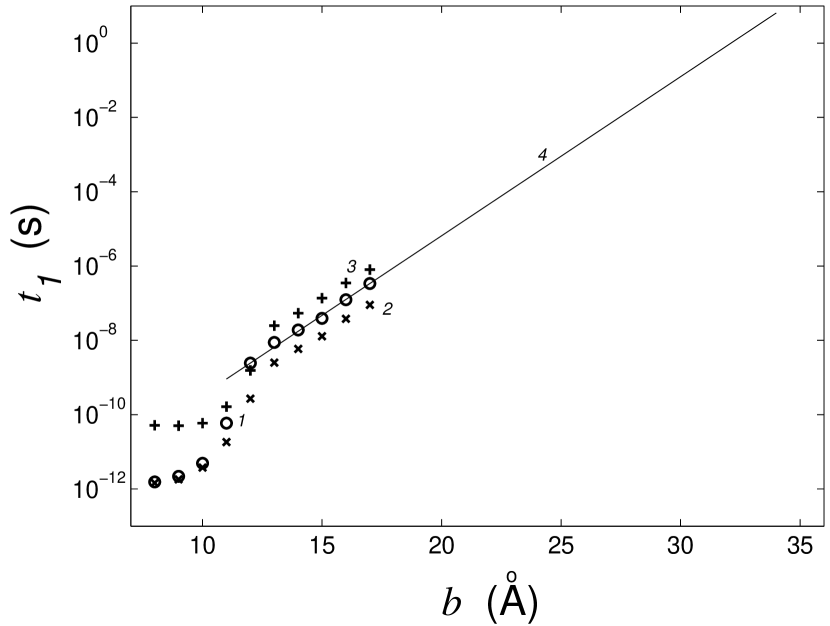
Figure 7: Gyro thermalization time $t_{1}$ computed as a function of molecular cavity diameter $b$ at $M=m$, $R_{0}=1$ Å (symbols 1); $M=m$, $R_{0}=\infty$ (symbols 2); $M=100m$, $R_{0}=\infty$ (symbols 3), and extrapolation of this function to large $b$ (curve 4).

V Conclusion

The molecular interfering gyroscope is a challenger for solving the kT-problem as a probable mechanism of magnetobiological effects. Indeed, the walls of a protein cavity do not interfere with the gyro degree of freedom directly via short-range chemical bonds. For cavities larger than 30 Å in size, the contribution to the relaxation from the van der Waals electromagnetic forces, induced by wall oscillations, is small. Radiation damping is negligibly small. Finally, the oscillations of gyro supports produce a zero moment of forces about the axis of rotation and do not affect the angular momentum. The gyro degree of freedom is very slow to thermalize, its dynamic behavior is coherent, which gives rise to slow interference effects. Of course, whether or not some more or less water-free cavities of the size of 30 Å and larger do exist remains an open question, but, what is essential, ELF magnetic field bioeffects are no longer a paradox.

The role of molecular gyros could probably be played by short sections of polypeptides and nucleic acids built inside globular proteins or in cavities between associated globules. In this respect it is interesting to look at Watson–Crick pairs of nitrous bases (adenine–thymine and guanine–cytosine) which bind DNA strands into a double helix as well as some other hydrogen-bound complexes of nitrous bases. Their rotations are hampered by steric factors. However, in the realm of activity of special DNA enzymes, steric constraints may be lifted to allow a relatively free rotation of molecular complexes. It is not yet clear whether or not the gyro type of molecular structures exists. They are unlikely to be detected by X-ray methods since these require crystallization of proteins for structural analysis. In this state, the rotation would likely be frozen. Should a rotation be allowed, the mobile groups would not give clear cut reflections. Some other methods are needed that would work with native forms of proteins avoiding distortions due to crystallization.

Generally speaking, the fact that the molecular gyro model gives a physically consistent explanation of MBEs proves indirectly its real grounds. Further studies should verify whether this conclusion is correct. In any case, today, the interfering molecular gyroscope is a single available mechanism to give explanations that would be physically transparent and generally agreeable with experiments.

References

- Blank (1995) M. Blank, ed., Electromagnetic fields: Biological Interactions and Mechanisms, Advances in Chemistry – 250 (Am. Chem. Soc., Washington, 1995).
- Goodman et al. (1995) E. Goodman, B. Greenebaum, and M. Marron, Int. Rev. Cytol. 158, 279 (1995).
- Bersani (1999) F. Bersani, ed., Electricity and Magnetism in Biology and Medicine (Kluwer/Plenum, London, 1999).
- Adey (1993) W. Adey, J. Cell Biochem. 51, 410 (1993).
- Belyaev et al. (1994) I. Belyaev, A. Matronchik, and Y. Alipov, in Charge and Field Effects in Biosystems – 4, edited by M. Allen (World Scientific, Singapore, 1994), pp. 174–184.
- Mullins et al. (1993) J. Mullins, D. Krause, and T. Litovitz, in Electricity and Magnetism in Biology and Medicine, edited by M. Blank (San Francisco Press Inc, San Francisco, 1993), pp. 345–346.
- Lin and Goodman (1995) H. Lin and R. Goodman, Bioelectroch. Bioener. 36, 33 (1995).
- Raskmark and Kwee (1996) P. Raskmark and S. Kwee, Bioelectroch. Bioener. 40, 193 (1996).
- Litovitz et al. (1997) T. Litovitz, M. Penafiel, D. Krause, D. Zhang, and J. Mullins, Bioelectromagnetics 18, 388 (1997).
- Binhi (1997) V. Binhi, Electro Magnetobiol. 16, 203 (1997).
- Binhi (1998) V. Binhi, Bioelectroch. Bioener. 45, 73 (1998).
- Binhi (2000) V. Binhi, Bioelectromagnetics 21, 34 (2000).
- Binhi et al. (2001) V. Binhi, Y. Alipov, and I. Belyaev, Bioelectromagnetics 22, 79 (2001).
- Binhi and Goldman (2000) V. Binhi and R. Goldman, Biochim. Biophys. Acta 1474, 147 (2000).
- Slichter (1980) C. Slichter, Principles of magnetic resonance (Springer, Berlin, 1980), 2nd ed.
- Landau and Lifshitz (1977) L. Landau and E. Lifshitz, Quantum Mechanics, vol. 3 of Theoretical Physics (Pergamon, Oxford, 1977).
- Liboff et al. (1987) A. Liboff, R. Rozek, M. Sherman, B. McLeod, and S. Smith, J. Bioelect. 6, 13 (1987).
- Ross (1990) S. Ross, Bioelectromagnetics 11, 27 (1990).
- Blackman et al. (1994) C. Blackman, J. Blanchard, S. Benane, and D. House, Bioelectromagnetics 15, 239 (1994).
- Garcia-Sancho et al. (1994) J. Garcia-Sancho, M. Montero, J. Alvarez, R. Fonteriz, and A. Sanchez, Bioelectromagnetics 15, 579 (1994).
- Blackman et al. (1995) C. Blackman, J. Blanchard, S. Benane, and D. House, FASEB J. 9, 547 (1995).
- Prato et al. (1995) F. Prato, J. Carson, K. Ossenkopp, and M. Kavaliers, FASEB J. 9, 807 (1995).
- Lednev et al. (1996a) V. Lednev, L. Srebnitskaya, E. Ilyasova, Z. Rozhdestvenskaya, A. Klimov, N. Belova, and H. Tiras, Biofizika 41, 815 (1996a).
- Lednev et al. (1996b) V. Lednev, L. Srebnitskaya, E. Ilyasova, Z. Rozhdestvenskaya, A. Klimov, and H. Tiras, Dokl. Ross. Akad. Nauk 348, 830 (1996b).
- Trillo et al. (1996) M. Trillo, A. Ubeda, J. Blanchard, D. House, and C. Blackman, Bioelectromagnetics 17, 10 (1996).
- Blackman et al. (1999) C. Blackman, J. Blanchard, S. Benane, and D. House, Bioelectromagnetics 20, 5 (1999).
- Noid et al. (1991) D. Noid, B. Sumpter, and B. Wunderlich, Macromolecules 24, 4148 (1991).
- Savin and Manevitch (1998) A. Savin and L. Manevitch, Phys. Rev. B 58, 11386 (1998).