On the nonlinear dynamics of topological solitons in DNA

Abstract

Dynamics of topological solitons describing open states in the DNA double helix are studied in the frameworks of the model which takes into account asymmetry of the helix. It is shown that three types of topological solitons can occur in the DNA double chain. Interaction between the solitons, their interactions with the chain inhomogeneities and stability of the solitons with respect to thermal oscillations are investigated.

I Introduction

It is widely accepted now that the DNA molecule has a rather moveable internal structure, and that the internal DNA mobility plays an important role in functioning the molecule. The thermal bath where the DNA molecule is usually immersed, collisions with the molecules of the solution which surrounds DNA, local interactions with proteins, drugs or some other ligands lead to activation of different types of internal motions. Small oscillations of individual atoms near equilibrium positions, rotational, transverse and longitudinal displacements of atomic groups (phosphate groups, sugars and bases), motions of the double chain fragments having several base pairs lengths, local unwinding of the double helix, transitions of DNA fragments from one conformational form to another, for example, from A-form to B-form and so on, are only some of them. A more detailed list of internal motions and of their dynamical characteristics can be found in the works of Fritzsche p1 , Keepers and co-authors p2 , McClure p3 , McCommon and co-authors p4 , Yakushevich p5 ; p6 ).

Different approaches to the modeling of the internal DNA mobility are known. One of them has been developed by Prohofsky and co-authors p7 ; p8 ; p9 ; p10 , who considered DNA as a lattice and took into account the motions of all atoms (except of hydrogen atoms) in the lattice cell. Their approach was limited, however, by harmonic approximation, and this limitation did not permit them to model large amplitude internal motions such as, for example, local unwinding of the double helix. Another approach, based on the methods of molecular dynamics and proposed firstly by Levitt p11 and Tidor and co-authors p12 , is known now as one of the most powerful tools of investigation of the internal DNA mobility p13 . This approach is not limited by harmonic approximation and therefore it can be used to study internal motions of both large and small amplitudes. The approach has, however, one essential deficiency: because of the limited possibilities of modern computers it can not be used to study long DNA fragments, and therefore it does not suitable for studies of the processes of propagation of local structural distortions along the molecule.

In this paper, to investigate the internal DNA mobility, we use the approach developed in a series of works p14 ; p15 ; p16 ; p17 ; p18 ; p19 ; p20 ; p21 ; p22 ; p23 ; p24 ; p25 . Peculiarity of the approach is that it uses rather simple models of the internal DNA dynamics, which take into account only one or a few types of the DNA internal motions. This simplification gives an opportunity to find analytical solutions of corresponding dynamical equations imitating both small and large amplitude internal motions. And one more merit of the approach is that it gives a possibility to study the internal dynamics of long DNA fragments. Three works in the series are of most interest.

The first one has been done by Englander and co-authors p14 who studied the dynamics of DNA open states. Their model took into account only rotational motions of nitrous bases, which as it was suggested, made the main contribution to formation of the open states. Another paper belonged to Peyrard and Bishop p22 , who studied the process of DNA denaturation. Suggesting that the stretching of the hydrogen bonds in pairs made the most contribution into the process, they created a simplified model where only transverse motions of bases along the direction of the hydrogen bonds where taken into account. The third important paper was published by Muto and co-authors p21 . These authors suggested that two types of internal motions were made the main contribution to DNA denaturation process: transverse motions along the hydrogen bond direction and longitudinal motions along the backbone direction. Their model consisted of two polynucleotide strands linked together through the hydrogen bonds described by a Lennard-Jones potential, and the phosphodiester bridges in the backbone were described by an anharmonic Toda potential.

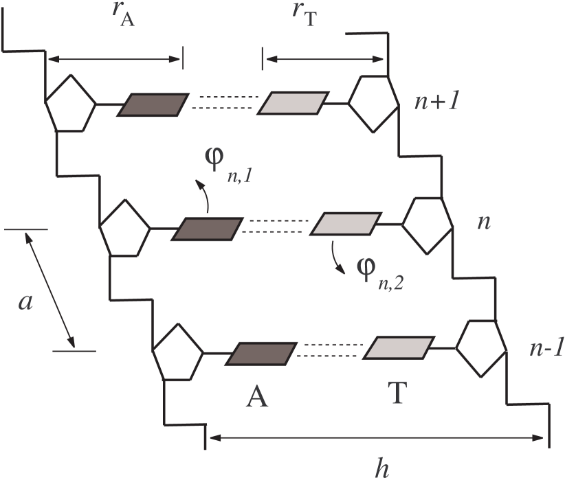
Figure 1: Fragment of the DNA double chain consisting of 3 AT base pairs. Longitudinal pitch of the helix $a=3.4$ Å;  transverse pitch $h=16.15$ Å.

Further development of the approach was limited for several years by small improvements of the models and their combinations, and only involving numerical methods of simulation of the internal DNA dynamics gave a new impulse and interesting possibilities which have been realized in the works of Van Zandt p26 , Techera and co-authors p27 , Salerno p25 , Barbi p28 ; p29 , and Campa p30 . Just these methods permitted not only to study a possibility of appearance of large amplitude localized distortions in the DNA structure, but also to investigate their stability, the influence of thermal noise, the interactions between the distortions, the propagation of them along the homogeneous and inhomogeneous DNA.

Table 1: The values of the parameters $m_{\alpha}$, $r_{\alpha}$, $I_{\alpha}=m_{\alpha}r_{\alpha}^{2}$, for all possible bases $\alpha$ ($m_{p}=1.67343\cdot 10^{-27}$ kg is the proton mass).

$\alpha$	$m_{\alpha}$ $(m_{p})$	$r_{\alpha}$ (Å)	$I_{\alpha}$ ($\times 10^{-47}$ m2kg)
A	135.13	5.8	7607.03
T	126.11	4.8	4862.28
G	151.14	5.7	8217.44
C	111.10	4.7	4106.93

In all these works, however, the asymmetry of the base pairs was neglected. That is both bases in a pair were modeled as identical structural elements with the same characteristics (masses, moments of inertia and so on). But even in the case of homogeneous (synthetic) DNA the asymmetry exists. Indeed, if, for example, one of the polynucleotide chains consists of only adenines, the other chain should consist of thymines, and this homogeneous model is substantially asymmetrical. Just this type of asymmetrical model is studied in this work. To simplify calculations, we consider only rotational motions of nitrous bases around the sugar-phosphate chains in the plane perpendicular to the main axis of the double chain. We find solitary wave solutions describing open states in the double helix. We classify the solitons, investigate stability of the solitons with respect to thermal oscillations, interactions between the solitons, interaction of the solitons with inhomogeneities of the chain. To solve all these problems, we use numerical-variation methods efficiency of which was proved in the works p31 ; p32 ; p33 ; p34 ; p35 ; p36 , devoted to the analysis of nonlinear dynamics of molecular chains and polymer crystals.

II Discrete model of the DNA double helix

Let us consider B-form of the DNA molecule, the fragment of which is presented in Fig. 1. The lines in the figure correspond to the skeleton of the double helix, black and grey rectangles correspond to bases in pairs (AT and GC). Let us focus our attention on the rotational motions of bases around the sugar-phosphate chains in the plane perpendicular to the helix axis. Below we shall call the chain placed on the left by the first chain, and the right chain – by the second one. Positive directions of the rotations of the bases for each of the chains are shown in Fig. 1.

Let us consider the plane DNA model where the chains of the macromolecule form two parallel straight lines placed at a distance $h$ from each other, and the bases can make only rotation motions around their own chain, being all the time perpendicular to it. Let us suggest that $\varphi_{n,1}$ is the angular displacement of the $n$-th base of the first chain, and $\varphi_{n,2}$ is the angular displacement of the $n$-th base of the second chain. Then the Hamiltonian of the double chain takes the form

$$H=\sum_{n}\left\{\frac{1}{2}I_{n,1}\dot{\varphi}_{n,1}^{2}+\frac{1}{2}I_{n,2}\dot{\varphi}_{n,2}^{2}+\epsilon_{n,1}\sin^{2}\frac{\varphi_{n+1,1}-\varphi_{n,1}}{2}+\epsilon_{n,2}\sin^{2}\frac{\varphi_{n+1,2}-\varphi_{n,2}}{2}+V_{\alpha\beta}(\varphi_{n,1},\varphi_{n,2})\right\}~{}.$$ (1)

The first two terms of Hamiltonian (1) correspond to the kinetic energy of the $n$-th base pair. Here $I_{n,1}$ is the moment of inertia of the $n$-th base of the first chain; $I_{n,2}$ is the moment of inertia of the $n$-th base of the second chain, point denotes differentiation in time $t$. For the base pair $\alpha\beta$ $(\alpha\beta=AT,~{}TA,~{}CG,~{}GC)$ the moment of inertia is equal to $I_{n,1}=m_{\alpha}r_{\alpha}^{2}$, $I_{n,2}=m_{\beta}r_{\beta}^{2}$. The value of the base mass $m_{\alpha}$, the length $r_{\alpha}$ and corresponding moment of inertia $I_{\alpha}=m_{\alpha}r_{\alpha}^{2}$ for all possible base pairs are presented in the Table 1.

The third and the fourth terms in Hamiltonian (1) describe interaction of the neighboring bases along each of the macromolecule chains. Parameter $\epsilon_{n,i}$ characterizes the energy of interaction of the $n$-th base with the $(n+1)$-th base of the $i$-th chain $(i=1,2)$. The value of the parameter is unknown. But if we take into account that angular displacement of one base is accompanied not only by overcoming the barrier due to the stacking interaction, but also by substantial deformation of the dihedral and valence angles,we can suggest that the energy of the displacement $\epsilon_{n,i}$ should be wittingly more than the stacking $40\div 60$ kJ/mol p37 , and it should weakly depend on the type of the base. This gives us a possibility to suggest later on that $\epsilon_{n,1}\equiv\epsilon_{n,2}\equiv\epsilon>60$ kJ/mol.

The fifth term in Hamiltonian (1) corresponds to the energy of interaction between conjugated bases of different chains. Here index $\alpha\beta=$AT, TA, GC, CG determines the type of the base pair. It is convenient to model the energy of interaction of conjugated pairs by the potential

$$V_{\alpha\beta}(\varphi_{n,1},\varphi_{n,2})=\frac{1}{2}K_{\alpha\beta}|{\bf R}_{n}-{\bf R}_{n}^{\circ}|^{2}~{},$$ (2)

where R_n is the vector connecting the end of the base $(n,1)$ with the end of the base $(n,2)$, R${}_{n}^{\circ}$ is the value of the vector for the ground state of the chain $\varphi_{n,1}\equiv 0$, $\varphi_{n,2}\equiv 0$. Potential (2) can be written in a more simple form

$$V_{\alpha\beta}(\varphi_{n,1},\varphi_{n,2})=K_{\alpha\beta}\{r_{\alpha}(r_{\alpha}+r_{\beta})(1-\cos\varphi_{n,1})+r_{\beta}(r_{\alpha}+r_{\beta})(1-\cos\varphi_{n,2})-r_{\alpha}r_{\beta}[1-\cos(\varphi_{n,1}-\varphi_{n,2})]\}~{}.$$ (3)

The rigidity of interaction $K_{\alpha\beta}$ can be estimated from the energy of interaction

$$e_{\alpha\beta}=\frac{1}{2}\left[V_{\alpha\beta}(0,\frac{\pi}{2})+V_{\alpha\beta}(\frac{\pi}{2},0)\right]=\frac{1}{2}K_{\alpha\beta}[r_{\alpha}^{2}+r_{\beta}^{2}]~{}.$$

The pair AT (TA) is stabilized by two hydrogen bonds (they are shown in Fig. 1 by dotted lines), and the pair CG (GC) – by three hydrogen bonds. Therefore we suggest later on that $e_{AT}=e_{TA}=2e_{CG}/3=2e_{GC}/3=e$.

For the value of the energy of interaction of the bases in AT base pair we can take the double energy of hydrogen bond $e=40$ kJ/mol. Then the rigidity of the bond between the bases is equal to

$$K_{AT}=K_{TA}=\frac{2}{3}K_{GC}=\frac{2}{3}K_{CG}=$$

$$K=\frac{2e}{r_{\alpha}^{2}+r_{\beta}^{2}}=0.234\mbox{ N/m}.$$ (4)

On the other hand, the value of the parameter can be estimated from the frequency spectrum of low amplitude oscillations of the chain. We shall obtain it in the next section.

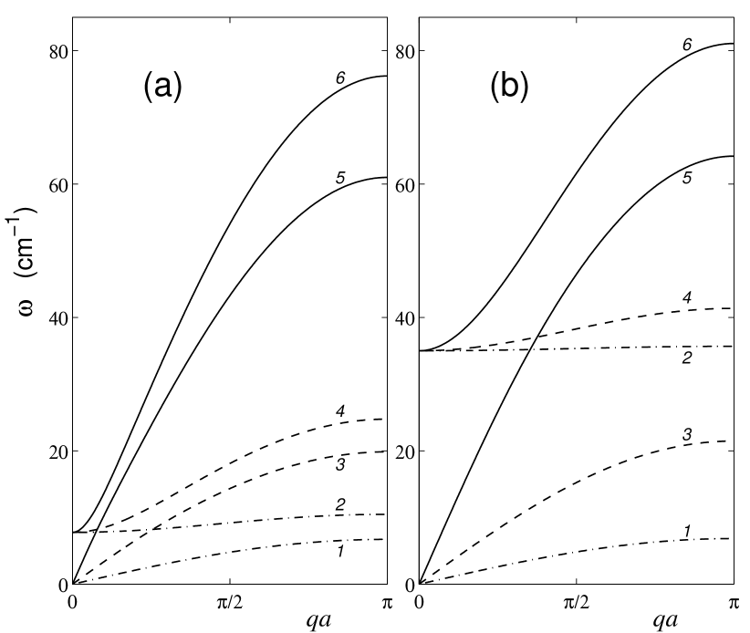
Figure 2: Acoustic $\omega=\omega_{a}(q)$ (curve 1, 3, 5) and optical $\omega=\omega_{o}(q)$ (curve 2, 4, 6) branches of the dispersion curve for homogeneous chain ($\alpha\beta=$AT, $\epsilon=$60, 600, 6000 kJ/mol) for chain with $K=0.234$ N/m (a) and $K=4.744$ N/m (b).

III Dispersion equation

The system of equations of motion, which corresponds to macromolecule Hamiltonian (1), takes the form

$$I_{n,1}\ddot{\varphi}_{n,1} = -\frac{\partial H}{\partial\varphi_{n,1}}~{};$$

$$I_{n,2}\ddot{\varphi}_{n,2} = -\frac{\partial H}{\partial\varphi_{n,2}}~{},$$ (5)

$$n = 0,\pm 1,\pm 2,...~{}~{}.$$

Let us consider homogeneous macromolecule where only one type of base pairs exists $\alpha\beta$ ($I_{n,1}\equiv I_{\alpha}$, $I_{n,2}\equiv I_{\beta}$).

Insert small amplitude plane wave

$$(\varphi_{n,1}(t),\varphi_{n,2}(t))=(\varphi_{1},\varphi_{2})Ae^{i(qan-\omega t)}~{},$$

into the system of equations (5). Here $(\varphi_{1},\varphi_{2})$ is a normalized to 1 two dimension vector, $A\ll\pi$ is the amplitude, $q\in[0,\pi/a]$ is the wave number. It is easy to show that in the linear approximation the frequency $\omega$ should satisfy the dispersion equation

$$\omega^{4}+B\omega^{2}+C=0~{},$$ (6)

where

$$B = [K_{\alpha\beta}(I_{\alpha}r_{\beta}^{2}+I_{\beta}r_{\alpha}^{2})+4\kappa(I_{\alpha}+I_{\beta})\sin^{2}\frac{qa}{2})]/I_{\alpha}I_{\beta}~{};$$

$$C = [4\kappa K_{\alpha\beta}(r_{\alpha}^{2}+r_{\beta}^{2})\sin^{2}\frac{qa}{2}+16\kappa^{2}\sin^{4}\frac{qa}{2}]/I_{\alpha}I_{\beta}~{},$$

$\kappa=\epsilon/2$ is the rigidity of the interaction of neighboring bases along the chain.

Dispersion curve (6) has two branches:

$$\omega_{a}(q) = [(B-\sqrt{B^{2}-4C})/2]^{1/2}~{};$$

$$\omega_{o}(q) = [(B+\sqrt{B^{2}-4C})/2]^{1/2}~{}.$$

The upper curve $\omega=\omega_{o}(q)$ corresponds to optical phonons, the lower curve $\omega=\omega_{a}(q)$ corresponds to acoustic phonons in the chain.

The frequency $\omega_{a}(q)$ tends to zero as $q\rightarrow 0$. Let us determine the velocity of acoustic phonons as

$$v_{0}=\lim_{q\rightarrow 0}\frac{\omega(q)}{q}=a\sqrt{\frac{\kappa(r_{\alpha}^{2}+r_{\beta}^{2})}{I_{\alpha}r_{\beta}^{2}+I_{\beta}r_{\alpha}^{2}}}~{}.$$

The dependence of the sound velocity $v_{0}$ in the homogeneous molecule $\alpha\beta=$AT (GC) on the energy of rotation $\epsilon$ is presented in the Table 2.

According to different estimations p38 ; p39 ; p40 the velocity of sound in DNA is on the interval from 1890 m/s till 3500 m/s. From the Table 2 it is clear, that among three typical values $\epsilon=60$, 600, 6000 kJ/mol the value $\epsilon=6000$ kJ/mol is the best one. Just this value will be used in the numerical investigations of the dynamics of topological solitons.

Table 2: Dependence of sound velocity $v_{0}$ (m/s) on the value of the parameter $\epsilon$ for homogeneous $\alpha\beta=$AT (GC) chain

$\epsilon$ (kJ/mol)	60	600	6000
AT	219.47	694.02	2194.7
GC	223.38	706.39	2233.4

The lowest value of the optical frequency is

$$\omega_{o}(0)=\sqrt{K_{\alpha\beta}(I_{\alpha}r_{\beta}^{2}+I_{\beta}r_{\alpha}^{2})/I_{\alpha}I_{\beta}}~{}.$$ (7)

According to p41 $\omega_{o}(0)=35$ cm^-1, therefore from (7) we have

$$K_{AT}=K=4.744\mbox{ N/m},~{}~{}K_{CG}=\frac{3}{2}K=7.117\mbox{ N/m}.$$ (8)

This estimation of the value of the rigidity differs from that obtained in (4). The use of the value given in (4) gives substantially lower value of the frequency $\omega_{o}(0)=7.77$ cm^-1. Thus we have the following estimation of the value of the parameter $K$: $0.234\leq K\leq 4.744$ N/m. The view of the dispersion curves for homogeneous chain ($\alpha\beta=AT$) with different values of the parameters is presented in Fig. 2.

For numerical investigation of the soliton dynamics we shall take intermediate value $K=0.8714$ N/m which corresponds to the frequency $\omega_{o}(0)=15$ cm^-1, and energy of interaction $e_{AT}=149$ kJ/mol.

IV Numerical method of finding solitary wave solutions

Complexity of the system of equations of motions (5) does not permit us to carry out analytical investigation. Therefore, we shall study it numerically and use variation technique, proposed in p32 , to find soliton like solutions.

Let us consider homogeneous DNA molecule (for all $n$ $I_{n,1}=I_{\alpha}$, $I_{n,2}=I_{\beta}$, where $\alpha\beta=$ AT (TA, CG, GC)). We shall find the solution of system (5) in the form of a wave with smooth constant profile. For the purpose, let us suggest that $\varphi_{n,1}(t)=\varphi_{1}(\xi)$, $\varphi_{n,2}(t)=\varphi_{2}(\xi)$, where the wave variable $\xi=na-vt$, and $v$ is the velocity of the wave.

Let us assume, that the functions $\varphi_{1}$ and $\varphi_{2}$ smoothly depend on $\xi$. Then the time second derivatives can be substituted for discreet derivatives

$$\frac{d^{2}\varphi_{n,i}}{dt^{2}}=v^{2}\frac{\partial\varphi_{i}}{\partial\xi^{2}}=v^{2}(\varphi_{n+1,i}-2\varphi_{n,i}+\varphi_{n-1,i})/a^{2},$$ (9)

$i=1,2$. Using these relations, we can write the equations of motions (5) in the form

$$L_{\varphi_{n,1}}=0,~{}~{}L_{\varphi_{n,2}}=0,~{}~{}n=0,\pm 1,\pm 2,...~{}.$$ (10)

Here the functional

$$L=\sum_{n}\{\frac{v^{2}}{2a^{2}}[I_{\alpha}(\varphi_{n+1,1}-\varphi_{n,1})^{2}+I_{\beta}(\varphi_{n+1,2}-\varphi_{n,2})^{2}]-$$

$$-\epsilon(\sin^{2}\frac{\varphi_{n+1,1}-\varphi_{n,1}}{2}+\sin^{2}\frac{\varphi_{n+1,2}-\varphi_{n,2}}{2})$$

$$-V_{\alpha\beta}(\varphi_{n,1},\varphi_{n,2})\}$$

is a discreet version of the Lagrangian

$${\cal L}=\sum_{n}[\frac{1}{2}I_{n,1}\dot{\varphi}_{n,1}^{2}+\frac{1}{2}I_{n,2}\dot{\varphi}_{n,2}^{2}-$$

$$-\epsilon(\sin^{2}\frac{\varphi_{n+1,1}-\varphi_{n,1}}{2}+\sin^{2}\frac{\varphi_{n+1,2}-\varphi_{n,2}}{2})$$

$$-V_{\alpha\beta}(\varphi_{n,1},\varphi_{n,2})]~{},$$

which corresponds to the system of equations of motion (5).

For further analysis it is convenient to write the functional $L$ in the dimensionless form

$$\bar{L}=2L/K(r_{A}^{2}+r_{T}^{2})=$$

$$\sum_{n}[c_{\alpha}(\varphi_{n+1,1}-\varphi_{n,1})^{2}+c_{\beta}(\varphi_{n+1,2}-\varphi_{n,2})^{2}$$

$$-g(\sin^{2}\frac{\varphi_{n+1,1}-\varphi_{n,1}}{2}+\sin^{2}\frac{\varphi_{n+1,2}-\varphi_{n,2}}{2})$$ (11)

$$-U_{\alpha\beta}(\varphi_{n,1},\varphi_{n,2})],$$

where the dimensionless coefficients

$$c_{\alpha}=\frac{v^{2}I_{\alpha}}{Ka^{2}(r_{A}^{2}+r_{T}^{2})},~{}~{}c_{\beta}=\frac{v^{2}I_{\beta}}{Ka^{2}(r_{A}^{2}+r_{T}^{2})},$$

parameter of cooperativity

$$g=2\epsilon/K(r_{A}^{2}+r_{T}^{2}),$$ (12)

dimensionless potential $U_{\alpha\beta}(\varphi_{n,1},\varphi_{n,2})=2V_{\alpha\beta}(\varphi_{n,1},\varphi_{n,2})/K(r_{A}^{2}+r_{T}^{2})$.

Soliton solution of the system (10) can be found numerically as a solution of the problem on conditional minimum

$$-\bar{L}\rightarrow\min_{\varphi_{2,i},...,\varphi_{N-1,i},~{}i=1,2}:$$ (13)

$$\varphi_{1,1}=\varphi_{-\infty,1},~{}\varphi_{1,2}=\varphi_{-\infty,2},$$ (14)

$$\varphi_{N,1}=\varphi_{\infty,1},~{}\varphi_{N,2}=\varphi_{\infty,2}~{}.$$ (15)

Boundary conditions (14), (15) for the problem (13) determine the type of the soliton solution. We should take a rather large number $N$, in order that the form of the solution of the problem might not depend on its value. For the purpose it is enough to take $N$ ten times larger than the width of the soliton.

The soliton solution of the problem (13) can be characterized by the topological charge q=$(q_{1},q_{2})$, where $q_{i}=(\varphi_{\infty,i}-\varphi_{-\infty,i})/2\pi$, $i=1,2$, is an integer $(q_{i}=0,\pm 1,\pm 2,...)$. To find soliton solution with topological charge q, it is necessary to solve the problem on minimum (13) with boundary conditions

$$\varphi_{-\infty,1}=\varphi_{-\infty,2}=0,~{}~{}\varphi_{\infty,1}=2\pi q_{1},~{}~{}\varphi_{\infty,2}=2\pi q_{2}~{}.$$

This problem was solved by the method of conjugated gradient. The value $N=2000$ was taken, and the initial point

$$\varphi_{n,i}=[1+\tanh\mu(n-N/2)]\pi q_{i}~{},~{}~{}i=1,2~{},$$

was used. Here $\mu$ is a changeable parameter.

Soliton solution (solution in the form of a solitary wave) $\{\varphi_{n,1}^{\circ},\varphi_{n,2}^{\circ}\}_{n=1}^{N}$ corresponds to topological soliton with the energy $E=K(r_{A}^{2}+r_{T}^{2})\bar{E}/2$, where dimensionless energy

$$\bar{E}=\sum_{n=1}^{N-1}[c_{\alpha}(\varphi_{n+1,1}-\varphi_{n,1})^{2}+c_{\beta}(\varphi_{n+1,2}-\varphi_{n,2})^{2}+$$

$$+g(\sin^{2}\frac{\varphi_{n+1,1}-\varphi_{n,1}}{2}+\sin^{2}\frac{\varphi_{n+1,2}-\varphi_{n,2}}{2})$$

$$+U_{\alpha\beta}(\varphi_{n,1}\varphi_{n,2})]$$

and with the diameter

$$D=1+2\sqrt{(n-\bar{n})^{2}p_{n}}~{},$$

where the point

$$\bar{n}=\sum_{n=1}^{N}np_{n}$$

determines the position of the soliton center, and the formula

$$p_{n}=\bar{E}_{n}/\bar{E}=\left\{\frac{1}{4}\left[c_{\alpha}(\varphi_{n+1,1}-\varphi_{n-1,1})^{2}+c_{\beta}(\varphi_{n+1,2}-\varphi_{n-1,2})^{2}\right]+\frac{1}{2}g\left[\sin^{2}\frac{\varphi_{n+1,1}-\varphi_{n,1}}{2}\right.\right.$$

$$\left.\left.+\sin^{2}\frac{\varphi_{n+1,2}-\varphi_{n,2}}{2}+\sin^{2}\frac{\varphi_{n,1}-\varphi_{n-1,1}}{2}+\sin^{2}\frac{\varphi_{n,2}-\varphi_{n-1,2}}{2}\right]+U_{\alpha\beta}(\varphi_{n,1}\varphi_{n,2})\right\}/\bar{E}$$

gives the distribution of the energy along the chain.

V Dynamical properties of solitons

At the beginning let us consider stationary soliton solutions of the problem (13). In the dimensionless functional $\bar{L}$, coefficients $c_{\alpha}=c_{\beta}=0$ when $v=0$. So, only one dimensionless parameter $g$ (12) which characterizes cooperativity of rotational motions remains in functional (11). The existence of soliton solution and its form depend on the value of the parameter.

V.1 Stationary solution

The results of numerical investigations of the problem (13) show that in the homogeneous chains stationary topological soliton solutions exist when the parameter of cooperativity $g$ is larger than the threshold value: $g\geq g_{0}>0$. The absence of the soliton topological stability when $g<g_{0}$ can be explained in the following way. Any topological defect can be eliminated by turning the DNA bases. The turning of one base about 360 degrees transfers the system to the initial state, that is $\phi_{i,n}\equiv\phi_{i,n}\pm 2\pi$. And this is why the narrow solitons with the size equal to one link of the chain are equivalent to the ground state and this is why they are unstable. So, only relatively wide solitons with the general turning consisting of several small changes of rotational angles that is when $|\phi_{i,n+1}-\phi_{i,n}|\ll 2\pi$, are stable. Dependence of the threshold value $g_{0}$ on the soliton topological charge q for homogeneous AT and GC chains are given in the Table 3.

Table 3: Dependence of the threshold value of the parameter of cooperativity $g_{0}$ on the value of the soliton topological charge q$=(q_{1},q_{2})$ for homogeneous $\alpha\beta=$AT (GC) chain

$(q_{1},q_{2})$	(1,0)	(0,1)	(1,1)
AT	8.3	5.7	8.3
GC	12.0	8.2	12.0

Table 4: Dependence of the energy $E$ and the diameter $D$ of stationary topological soliton on its topological charge q with two values of the transverse rigidity $K$

		$\alpha\beta=$AT		$\alpha\beta=$GC
$K$ (N/m)	q	$E$ (kJ/mol)	$D$	$E$ (kJ/mol)	$D$
	(1,0)	2776.52	16.59	3405.48	13.69
0.234	(0,1)	2237.36	19.58	2733.60	16.18
	(1,1)	4971.72	42.85	6087.54	35.13
	(1,0)	5329.76	9.03	6394.96	7.64
0.8714	(0,1)	4302.09	10.59	5146.38	8.98
	(1,1)	9551.14	22.60	11444.96	18.93

From Fig. 3 it becomes clear that the soliton energy $\bar{E}$ and its width $D$ monotonously increase when the parameter of cooperativity $g$ increases. For soliton stability it is necessary that its width $D>4.33$. The view of stationary solitons with the parameters of cooperativity $g=10$ and $g=150$ is presented in Fig. 4. In the case of the soliton with topological charge q=(1,0), the first component has the form of a smooth step (when $n$ monotonously changes, the base of the first of two DNA chains makes a complete turn) accompanied by smooth small amplitude deformation in the second component (Fig. 4a). In the case of the soliton with q=(0,1), only the second component has the form of a step (Fig. 4b). In the case of soliton with q=(1,1), each of the components has the form of a step (Fig. 4c), steps being displaced relatively one another. Later on we shall show that this soliton is the bound state of two topological solitons with the charges q₁=(1,0) and q₂=(0,1). There exist two equivalent states of the soliton: the left state q=(1,1)_l, when the soliton with the charge q₁ is on left of the soliton with the charge q₂ (Fig. 4c), and the right state q=(1,1)_r, when the soliton with the charge q₁ is on right of the soliton with the charge q₂.

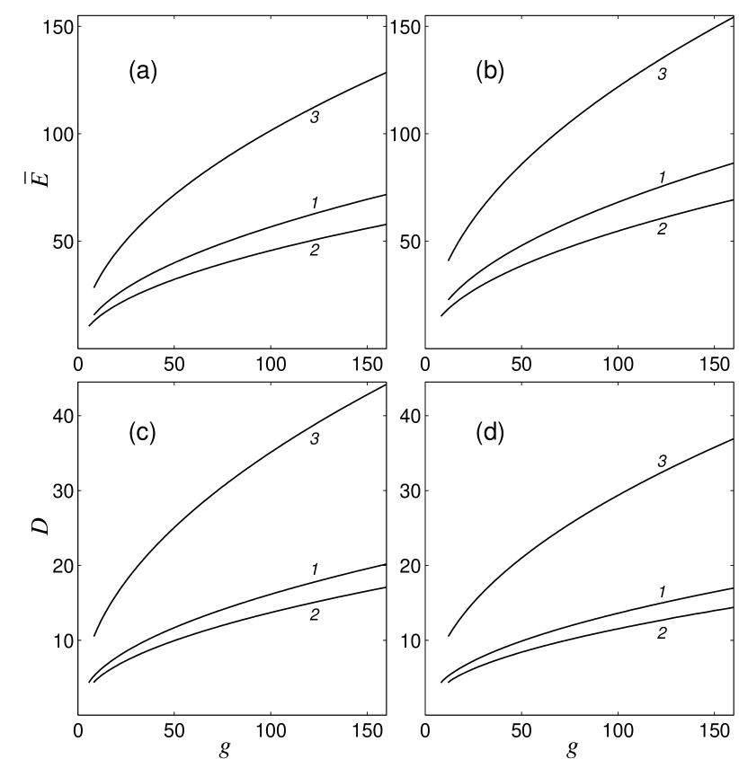
Figure 3: Dependence of the dimensionless soliton energy $\bar{E}$ and the width $D$ on the velue of the parameter of cooperativity $g$ when q=(1,0), (0,1), (1,1) (curves 1, 2, 3) in homogeneous AT (a),(c) and GC chains (b),(d).

When $\epsilon=6000$ kJ/mol and $K=0.234$ N/m the parameter of cooperativity $g=150.24\gg g_{0}$, and when $K=0.8714$ N/m the parameter $g=40.34>g_{0}$ (see Table 3) for all types of topological solitons. So, for these values of the rigidity parameter $K$ stable solitons with different topological charges exist. For maximum value of the rigidity parameter $K=4.744$ N/m the parameter of cooperativity $g=7.41<g_{0}$, and this means that stable topological solitons are absent. Thus the problem of the existence of topological solitons (open states) in the DNA reduces to the problem of receiving exact estimation of the parameters $\epsilon$ $K$. But this is, however, a rather difficult problem. We think that the values $\epsilon=6000$ kJ/mol, $K=0.8714$ N/m, when all three types of solitons exist, are the most grounded. And we shall use these values for further calculations.

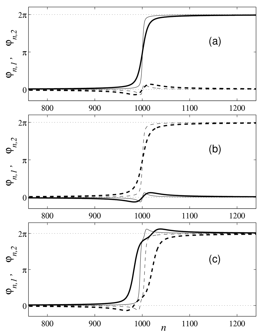
Figure 4: The view of stationary soliton with the topological charge q=(1,0) (a); q=(0,1) (b); q=(1,1)_l (c). Continuous lines correspond to displacements by the first component $\varphi_{n,1}$; dotted lines – to displacements by the second component $\varphi_{n,2}$; thin lines correspond to chain with $g=10$; flat lines – to chain with $g=150$.

Dependence of the energy $E$ and the diameter $D$ of stationary topological soliton on its topological charge q in the chain with $\epsilon=6000$ kJ/mol and the transverse rigidity determined by formulas (4) and (8), are given in the Table 4. From the data of the table it follows that the energy of the interaction of the solitons with the charges (1,0) and (0,1) is equal to $\Delta E=E(1,0)+E(0,1)-E(1,1)=90.71$ kJ/mol for the chain with the rigidity of the transverse interaction $K=0.8714$ N/m, and the energy is equal to $\Delta E=42.16$ kJ/mol for the chain with $K=0.234$ N/m.

V.2 Nonstationary solutions

Numerical investigation of the problem (13) shows, that in the homogeneous chain, topological soliton has the interval of the velocities $0\leq s\leq s_{1}<1$, where $s=v/v_{0}$ is the dimensionless velocity and $v_{0}$ is the velocity of sound. Dependence of maximum velocity of the soliton $s_{1}$ on its charge q, on type of the base in the chain $\alpha\beta$ and on the rigidity of the transverse interaction $K$ is presented in the Table 5.

Table 5: Dependence of the maximum value of the soliton velocity $s_{1}$ on its topological charge q, the soliton moving in the homogeneous $\alpha\beta$ chain with the transverse rigidity $K$.

$K$ (N/m)	q	AT	GC
	(1,0)	0.77	0.70
0.234	(0,1)	0.88	0.84
	(1,1)	0.77	0.70
	(1,0)	0.64	0.55
0.8714	(0,1)	0.86	0.84
	(1,1)	0.65	0.56

Dependence of the soliton energy $E$ and the diameter $D$ on the dimensionless velocity $s$ is presented in Fig. 5. With the increasing of the soliton velocity its energy monotonically increases, and the diameter monotonically decreases. Using the dependence $E(s)$ we can find the mass of rest of the topological soliton

$$M=\lim_{s\rightarrow 0}\frac{2(E(s)-E(0))}{s^{2}v_{0}^{2}}~{}.$$

Dependence of the mass of rest $M$ of the soliton on its charge q, on the type of the bases of the chain $\alpha\beta$ and on the rigidity of the transverse interaction $K$ is presented in the Table 6.

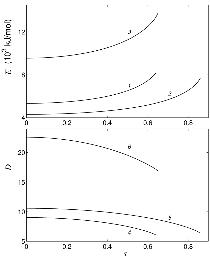
Figure 5: Dependence of the energy $E$ and the diameter $D$ of the soliton which moves along homogeneous AT chain and has the charge q$=(1,0)$ (curves 1 and 4), q$=(0,1)$ (curves 2 and 5) and q$=(1,1)$ (curves 3 and 6), on the dimensionless velocity $s$ ($\epsilon=6000$ kJ/mol, $K=0.8714$ N/m).

Table 6: The dependence of the soliton mass of rest $M$ (the values are given in proton mass units $m_{p}$) on its topological charge q, the soliton being in the homogeneous $\alpha\beta$ chain with the transverse rigidity $K$.

$K$ (N/m)	q	AT	GC
	(1,0)	7640	9663
0.234	(0,1)	4052	4064
	(1,1)	11581	13590
	(1,0)	14978	18730
0.8714	(0,1)	7899	7804
	(1,1)	22660	26265

Numerical investigation shows that all topological solitons at all permitted velocities are stable. They move along the chain with constant velocity, their form and energy being conserved. Thus, the specificity of the chain of the DNA molecule leads to a principal effect consisting in the possibility of preferable localization of soliton excitations on one chain. Moreover, it appears that soliton excitation with the charge (1,1) is a bound state of two excitations localized in separate chains.

VI Interaction of topological solitons

DNA is a rather long molecule, and several open states can be activated in it simultaneously. Therefore it is interesting to consider the problem of interaction of solitons imitating the open states.

Numerical approach (13) permits us to investigate the problem and to obtain the dependence of the energy of a pair of solitons with the charges q₁, q₂ on the distance between their centers $n_{1}$, $n_{2}$. For the purpose, it is necessary to take the boundary conditions and the initial point, which correspond to a pair of topological solitons with the centers moving away at a distance $R$. When minimizing the energy of the system $E=-L$, it is necessary also to fix the turns of the bases, which correspond to the centers of solitons. Then the energy of the obtained state $E(R)$ corresponds to the energy of a pair of topological solitons, the solitons being at a distance $R=n_{2}-n_{1}$ from each other. By changing positions of the soliton centers, we can obtain the potential of interaction

$$U_{{\bf q}_{1},{\bf q}_{2}}(R)=E(R)-E({\bf q_{1}})-E({\bf q_{2}})~{},$$

where $E({\bf q_{1}})$ and $E({\bf q_{2}})$ is the energy of isolated solitons.

The potential of interaction of solitons of different types and the potential of topological solitons with the charges of the same sign are presented in Fig. 6. The potential of two solitons of different types with q${}_{1}=(1,0)$ and q${}_{2}=(0,1)$ has the form of symmetrical double well potential (Fig. 6, curve 1). Maximum of the potential is reached when $R=0$, that is when the centers of the solitons are placed at the neighboring chains and when the solitons are opposite to each other. From energetic point of view this configuration of the solitons of different chains is the most disadvantageous. Minimum of the energy is reached when $R=\pm 20a$. Thus two solitons of this type can form two energetically equivalent coupled states. One of the states (left minimum of the potential of interaction) corresponds to the left isomer of the topological soliton with the charge q$=(1,1)_{l}$, and the other state (the right minimum of the potential of interaction) corresponds to the right isomer of the soliton ${\bf q}=(1,1)_{r}$.

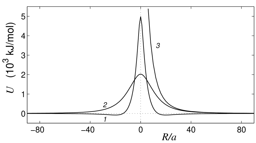
Figure 6: Potential of interaction of solitons $U_{{\bf q}_{1},{\bf q}_{2}}(R)$ with q${}_{1}=(1,0)$, q${}_{2}=(0,1)$ (curve 1); q${}_{1}=(1,0)$, q${}_{2}=(0,-1)$ (curve 2); q${}_{1}={\bf q}_{2}=(1,0)$ and q${}_{1}={\bf q}_{2}=(0,1)$ (curve 3).

If solitons have different signs of charges q${}_{1}=(1,0)$ and q${}_{2}=(0,-1)$, the potential of interaction has a bell-like form with one maximum at $R=0$ (Fig. 6, curve 2). From the potential it follows that, the solitons which belong to different chains, should repulse from each other. Solitons with the same sign of charge (q${}_{1}={\bf q}_{2}=(1,0)$, (0,1)) also repulse from each other.

When distance between the solitons decreases, the energy monotonically increases and goes to infinity when $R\rightarrow 0$ (Fig. 6, curve 3).

The potential of interaction $U_{{\bf q}_{1},{\bf q}_{2}}(R)$ permits to predict the result of repulsion of solitons with the charges ${\bf q}_{1}$ and ${\bf q}_{2}$. Let us model the repulsion of the solitons. For the purpose, let us consider a double chain consisting of $N=4000$ base pairs. At the ends of each of the polynucleotide chains let us introduce viscous friction which provides with absorption of phonons. The system of equations of motion (5), $n=1,2,...,N$, was integrated numerically with the initial condition which corresponds to two topological solitons with the centers placed in the points $n_{1}=N/4$ and $n_{2}=3N/4$ and with the velocities $s_{1}=-s_{2}=s>0$.

The results show that collision of solitons having equal signs q${}_{1}={\bf q}_{2}=(\pm 1,0),~{}(0,\pm 1)$ leads to their reflection at one another. When the velocities $s$ are small, the reflection is practically elastic, and when the velocities $s$ are large, collision is accompanied by slight emission of phonons. Collision of solitons with q${}_{1}=(\pm 1,0)$, q${}_{2}=(0,\mp 1)$ and $s=0.5$ leads to their reflection, accompanied by slight emission of phonons. This behavior is in a good agreement with the form of corresponding potential of interaction (Fig. 6, curve 2). To pass through one another, solitons need to overcome energy barrier $U_{{\bf q}_{1},{\bf q}_{2}}(0)=2025$ kJ/mol. Thus, their kinetic energy should be equal to $E_{k}(s)=E_{{\bf q}_{1}}(s)+E_{{\bf q}_{2}}(s)-E_{{\bf q}_{1}}(0)-E_{{\bf q}_{2}}(0)>U_{{\bf q}_{1},{\bf q}_{2}}(0)$. This condition is fulfilled only in the vicinity of the most possible values of the velocity (see. Fig. 5). So, when $s=0.5$, the kinetic energy $E_{k}=1732$ kJ/mol is lower than the height of the energy barrier (reflection takes place), and when $s=0.6$, the energy $E_{k}=3000.9$ kJ/mol is higher than the barrier (solitons pass through one another).

Solitons with the charges q${}_{1}=(\pm 1,0)$, q${}_{2}=(0,\pm 1)$ attract one another at a distance $R>20a$, and when the distance is shorter they repulse one another. Here the energy barrier $U_{{\bf q}_{1},{\bf q}_{2}}(0)=4989$ kJ/mol does not permit solitons to pass through one another. Solitons always reflect. Formation of the bound state does not occur even when the value of the velocity is small. It is explained by small value of the bond energy $\Delta E=91$ kJ/mol.

Potential of interaction of different topological solitons with the charges of opposite signs $({\bf q}_{1}=-{\bf q}_{2})$ is presented in Fig. 7. Potential of interaction of one component solitons $({\bf q}_{1}=(1,0),~{}(0,1))$ monotonically decreases with the decreasing of the distance between the solitons. When $R\rightarrow 0$, the potential $U_{{\bf q}_{1},{\bf q}_{2}}(R)\rightarrow-[E({\bf q}_{1})+E({\bf q}_{2})]$. At a distance $R=0$ solitons completely recombine.

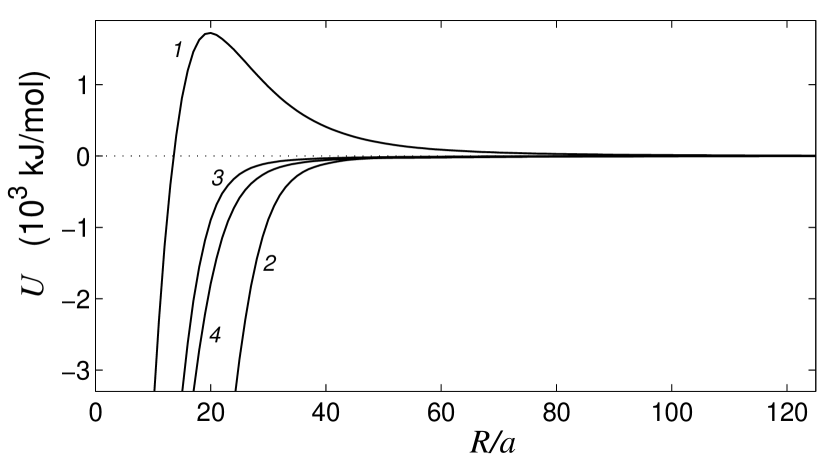
Figure 7: Potential of interaction of solitons $U_{{\bf q}_{1},{\bf q}_{2}}(R)$ with q${}_{1}=(1,1)_{l}$, q${}_{2}=(-1,-1)_{l}$ (curve 1); q${}_{1}=(1,1)_{l}$, q${}_{2}=(-1,-1)_{r}$ (curve 2); q${}_{1}=(1,0)$, q${}_{2}=(-1,0)$ (curve 3); q${}_{1}=(0,1)$, q${}_{2}=(0,-1)$ (curve 4).

Potential of interaction of two component solitons with the charges of different signs has a similar form. If the solitons have different polarity, that is, if the first soliton is a left isomer $({\bf q}_{1}=(1,1)_{l})$ and the second soliton is a right isomer $({\bf q}_{2}=(-1,-1)_{r})$. Solitons of that type attract one another. Their collisions always leads to recombination of the solitons.

If solitons have the same polarity, they repulse when $R>20a$, and attract when the distances are shorter. Recombination of the solitons requires overcoming the energy barrier 1730 kJ/mol. Solitons overcome the barrier only when $s>0.38$, and the value of their kinetic energy is more than the height of the barrier. When the value of the velocity is smaller, solitons reflect, and when the value is larger they recombine (Fig. 8). During recombination the energy of solitons is spent for intensive emission of phonons. Breather-like excitations can be also formed.

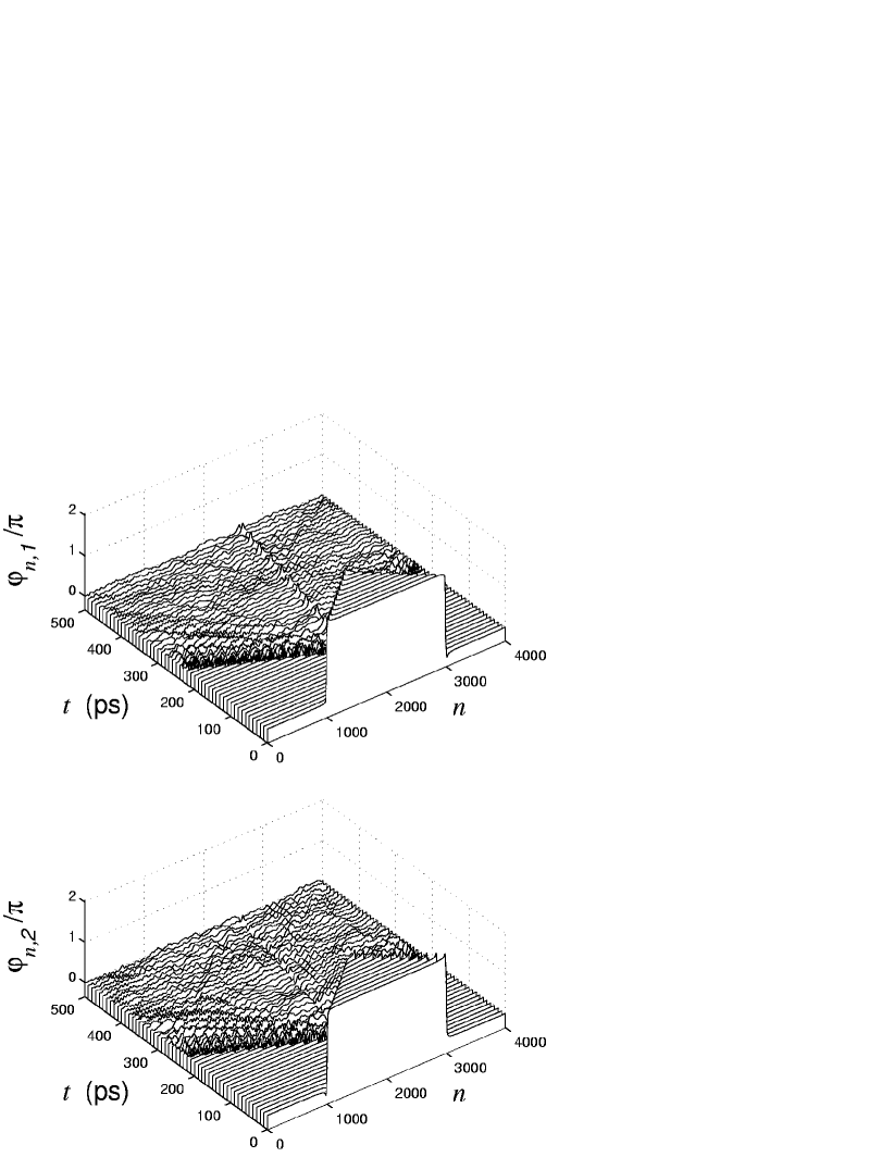
Figure 8: Recombination of solitons with the same signs of charges and the same polarities (${\bf q}_{1}=(1,1)_{l}$, ${\bf q}_{2}=(-1,-1)_{l}$, $s=0.5$).

Collision of one component soliton with two component soliton can lead (depending on the relationship of the signs of charges and on the polarity of the two component soliton) to their partial recombination or to inelastic reflection accompanied by disintegration of the two component soliton. So, at the velocity $s=0.5$ collision of the soliton having the charge ${\bf q}_{1}=(1,0)$, with the two component soliton having the charge ${\bf q}_{2}=(1,1)_{l}$, leads to inelastic reflection of the first soliton, and at the same time the second soliton disintegrates into two one component solitons with the charges (1,0) and (0,1) (Fig. 9).

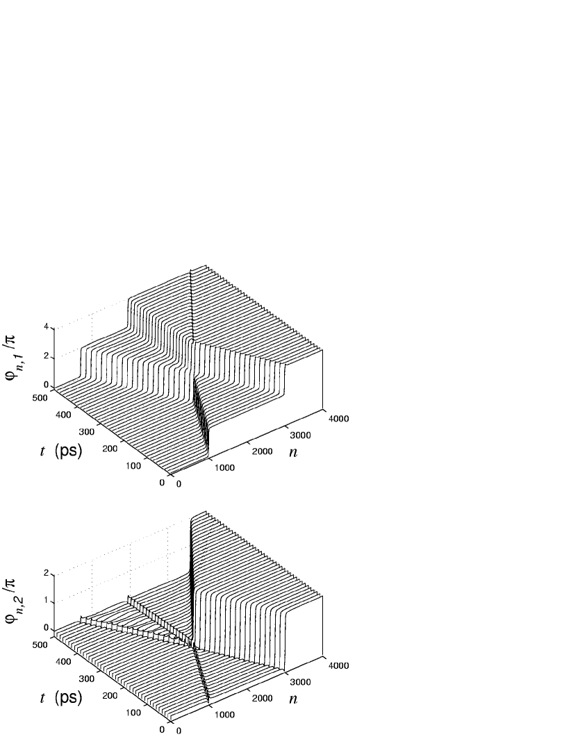
Figure 9: Disintegration of two component soliton (${\bf q}_{2}=(1,1)_{l})$ when it comes into collision with one component soliton (${\bf q}_{1}=(1,0))$. The velocity of the movement is $s=0.5$.

VII Effect of the chain inhomogeneities on the dynamics of topological solitons

Till now our investigation was limited by consideration of homogeneous model of DNA. The real DNA is, however, a substantially inhomogeneous system, therefore it is of special interest to consider the effect of the chain inhomogeneity on the dynamics of topological solitons. In the inhomogeneous chain, the energy of stationary soliton $E$ will depend on the position of the center of the soliton $\bar{n}$. To move, soliton requires to overcome the energetic potential barrier $E(\bar{n})$. To find the energy of the soliton with the center at the point $n=\bar{n}$ we need to solve numerically the problem of minimizing

$$E\rightarrow\min_{\varphi_{2,i},...,\varphi_{N-1,i},~{}i=1,2}:$$ (16)

$$\varphi_{1,1}=\varphi_{-\infty,1},~{}~{}\varphi_{1,2}=\varphi_{-\infty,2},$$ (17)

$$\varphi_{N,1}=\varphi_{\infty,1},~{}~{}\varphi_{N,2}=\varphi_{\infty,2},$$ (18)

where the energy

$$E=\sum_{n}[\epsilon(\sin^{2}\frac{\varphi_{n+1,1}-\varphi_{n,1}}{2}+\sin^{2}\frac{\varphi_{n+1,2}-\varphi_{n,2}}{2})$$

$$+V_{\alpha\beta_{n}}(\varphi_{n,1},\varphi_{n,2})],$$

$\alpha\beta_{n}$ – the sequence of the base pairs along the chain. The boundary conditions (17), (18) are the same as those in the problem (13). To fix the soliton center position we need to solve the problem of minimizing (16) with respect to variables $\varphi_{n,i}$ where $2\leq n\leq N-1$, $n\neq\bar{n}$, $i=1,2$. For soliton with charge $q_{1}\neq 0$ it is necessary to fix the value $\varphi_{\bar{n},1}=\pi q_{1}$, and for soliton with $q_{2}\neq 0$ – the value $\varphi_{\bar{n},2}=\pi q_{2}$.

The problem on conditional minimum (16) has been solved by the numerical method of conjugate gradient. We took $N=2000$. Possible view of energetic profile of the soliton moving in the inhomogeneous chain is presented in Fig. 10

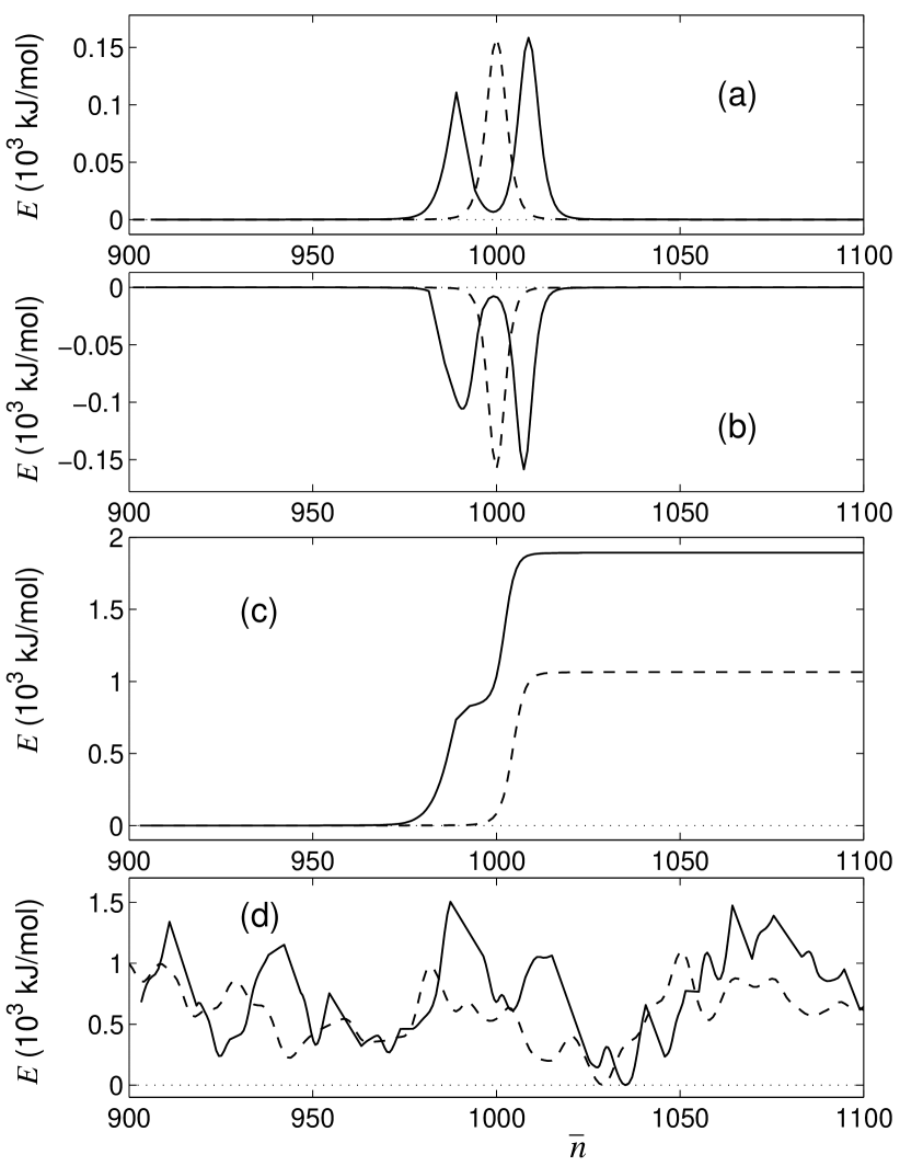
Figure 10: The view of energetic relief for soliton in the inhomogeneous chain: in homogeneous AT chain with one GC base pair (a); in homogeneous GC chain with one AT base pair (b); in the chain the first part of which consists of only AT base pairs, and the second - of only GC base pairs (c); in the chain with random sequence of base pairs (d). Dotted line shows the relief of the soliton with topological charge q$=(1,0)$, firm line – the relief for soliton with charge q$=(1,1)$.

At the beginning, let us estimate the effect of point inhomogeneities. From Fig. 10a it is obvious that one point defect in the homogeneous AT chain leads to appearance of localized potential barrier with height equal to $E_{d}=150$ kJ/mol. To overcome the barrier, the soliton kinetic energy should satisfy the condition $E_{k}(s)=E(s)-E(0)>E_{d}$. Soliton can to overcome the barrier only when its velocity $s>s_{d}$, where the threshold value of the velocity $s_{d}$ is taken from equation $E(s_{d})-E(0)=E_{d}$. From the data of Fig. 5 it is easy to find, that for soliton with q=(1,0) the velocity $s_{d}=0.21$, for soliton with q=(0,1) the velocity $s_{d}=0.28$, and when q=(1,1) the velocity $s_{d}=0.17$.

Let us model numerically the interaction of soliton with local defect of the homogeneous AT chain. For the purpose, let us consider homogeneous AT chain consisting of $N=4000$ bases with one base GC in the middle of the chain in the point $n=N/2$. Suggest that at the initial time a topological soliton is in the point $n=N/4$ and consider its movement through the chain inhomogeneity. The results of numerical modeling of the soliton dynamics show, that independently on the value of topological charge q soliton with velocity $s=0.05$ reflect from this point defect, but for $s=0.5$, moves through the point defect with negligibly small energy loss.

Point defect in the homogeneous GC chain leads to formation of localized potential well with depth 150 kJ/mol (see Fig. 10b). Almost at all values of the velocity soliton easily propagates along this chain without formation of bound state. Thus we can conclude that soliton moving in the DNA chain with sufficiently large velocity ($s>s_{d}$) is stable with respect to point defects.

In the chain one part of which consists of only AT base pairs, and the other – of only GC base pairs energetic barrier takes the form of smooth step (Fig. 10c). The height of the step is equal to the difference between the values of soliton energy in homogeneous GC and AT chains. From data of table 4 it follows, that the height of the step is equal to $\Delta E=1065$ kJ/mol for soliton with topological charge q=(1,0) and $\Delta E=844$ kJ/mol for soliton with q=(0,1), and when q=(1,1) the energy $\Delta E$=1894 kJ/mol. Soliton moving along homogeneous AT region of the chain, can enter into GC region only if its kinetic energy $E_{k}(s)>\Delta E$. As seen from Fig. 5, this condition is satisfied only if soliton velocity $s>s_{k}$, where the threshold value of the velocity is determined by the equation $E_{k}(s_{k})=\Delta E$. For soliton with q=(1,0) the velocity $s_{k}=0.48$, for q=(0,1) $s_{k}=0.59$, and for q=(1,1) the velocity $s_{k}=0.52$.

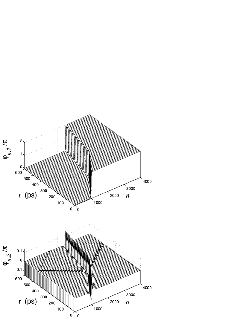
Figure 11: Movement of soliton with q$=(1,0)$, $s=0.5$ through the boundary between homogeneous AT and GC regions.

Let us model numerically the soliton moving from homogeneous AT region of the chain to homogeneous GC region. The results of the modeling show that the soliton with velocity $s=0.05<s_{k}$ and with any topological charge reflects elastically from the boundary between the regions. At given velocity the soliton kinetic energy is not large enough to overcome energetic barrier ($E_{k}(s)\ll\Delta E$). Soliton with $s=0.5$ ${\bf q}=(1,0)$ moves through the boundary between homogeneous regions and its motion is accompanied by emission of phonons. Inside the region consisting of GC base pairs, soliton continues to move, but with a smaller magnitude of the velocity (Fig. 11). For given value of q the threshold value of the velocity $s_{k}=0.48<0.5$. So, the kinetic energy of soliton is large enough to overcome energetic barrier. Because the main part of the kinetic energy is spent to overcome the barrier, the velocity of the soliton substantially decreases after overcoming the barrier. When q=(0,1) the threshold value of the velocity $s_{k}=0.59$ and soliton reflects at $s=0.5$ from the boundary of the homogeneous regions. The reflection is accompanied by phonon emission. For soliton with the charge q=(1,1) the velocity $s=0.5<s_{k}=0.52$ is not enough to overcome energetic barrier. Collision of soliton having topological charge $({\bf q}=(1,1)_{l})$ with the boundary between the homogeneous regions leads to the disintegration of the soliton. It disintegrates into two one component solitons with the charges ${\bf q}_{1}=(1,0)$ and ${\bf q}_{2}=(0,1)$. Soliton with the charge q₂ continues to move into GC region of the chain, and soliton with the charge q₁ reflects from the boundary.

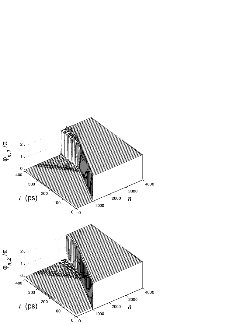
Figure 12: Entering two component soliton (charge q$=(1,1)_{l}$, velocity $s=0.5$) the random inhomogeneous region of the chain, and further disintegration of the soliton.

Let us consider the propagation of soliton in the inhomogeneous chain with random sequence of bases. In this case random energetic relief $E(n)$ is formed. The amplitude of the relief for soliton with q=(1,0) reaches 1000 kJ/mol, and for soliton with q=(1,1) – 1500 kJ/mol (Fig. 10d). It is obvious that uniform propagation of soliton in the chain of that type is impossible, because soliton loses part of energy for phonon emission when crossing each homogeneity.

Let us consider the movement of soliton through inhomogeneous region of the chain. For the purpose, let us suggest that the second part of the chain is formed by a random equal-possible sequence of base pairs AT, TA, CG, GC. The results of numerical modeling of the soliton dynamics show that soliton with small value of the velocity $s=0.05$ and with any topological charge reflects from the boundary of the inhomogeneous region. This points out, that penetration of the soliton into the inhomogeneous region requires the overcoming of some energy barrier. Soliton with larger velocity $s=0.5$ and charge q$=(1,0)$ overcomes this barrier, enters the disordered region of the chain and stops there. The movement in the disordered region is accompanied by intensive emission of phonons, which leads to the stop of the soliton. Soliton with q=$(0,1)$ can not overcome the barrier even at this value of the velocity. The soliton reflects from the boundary of the inhomogeneous region. The reflection is accompanied by emission of phonons. Two component soliton with q$=(1,1)_{l}$ enters inhomogeneous region, and at the same time it disintegrates into two one component solitons with the charges q${}_{1}=(1,0)$ and q${}_{2}=(0,1)$. The solitons moves some time in the inhomogeneous chain, then they stop (Fig. 12). The path of the solitons can reach several hundred base pairs.

Analogous results have been obtained even in the case when inhomogeneous region was formed by the base pairs AT and TA. Thus, the sequence of nitrous bases of DNA molecule should substantially influence the characteristics of the motion of topological soliton. Note, that it has been pointed out firstly in the work p25 .

VIII Interaction of topological solitons with thermal oscillations of the chain

Dynamics of a thermalized chain consisting of $N$ sites, is described by the system of the Langevin equations

$$I_{n,1}\ddot{\varphi}_{n,1} = -\frac{\partial H}{\partial\varphi_{n,1}}+\xi_{n,1}-\Gamma I_{n,1}\dot{\varphi}_{n,1}~{};$$

$$I_{n,2}\ddot{\varphi}_{n,2} = -\frac{\partial H}{\partial\varphi_{n,2}}+\xi_{n,2}-\Gamma I_{n,2}\dot{\varphi}_{n,2}~{},$$ (19)

$$n = 1,2,...N~{},$$

where the Hamiltonian of the system $H$ is given by Eq. (1), $\xi_{n,i}$ are random normally distributed forces describing the interaction of the $n$-th base of the $i$-th chain $(i=1,2)$ with thermal bath, $\Gamma=1/t_{r}$ is the coefficient of friction, $t_{r}$ being the relaxation time of the rotation velocity of one base. The random forces $\xi_{n,i}$ have normal distribution and the correlation functions are

$$\langle\xi_{n,i}(t_{1})\xi_{m,j}(t_{2})\rangle=2\Gamma k_{B}T\delta_{nm}\delta_{ij}\delta(t_{1}-t_{2})\sqrt{I_{n,i}I_{n,j}},$$

$$n,m=1,2,...,N,~{}~{}i,j=1,2~{}~{},$$

where $k_{B}$ is Boltzmann’s constant and $T$ is the temperature of thermal bath.

The system (19) was integrated numerically by the standard fourth-order Runge-Kutta method with constant step of integration $\Delta t$. The delta function was represented as $\delta(t)=0$ when $|t|>\Delta t/2$, and $\delta(t)=1/\Delta t$ when $|t|\leq\Delta t/2$, i.e., the step of numerical integration corresponded to the correlation time of the random force. In order to use the Langevin equation, it was necessary to suggest that $\Delta t\ll t_{r}$. Therefore we chose $\Delta t=0.001$ ps and the relaxation time $t_{r}\geq 1$ ps.

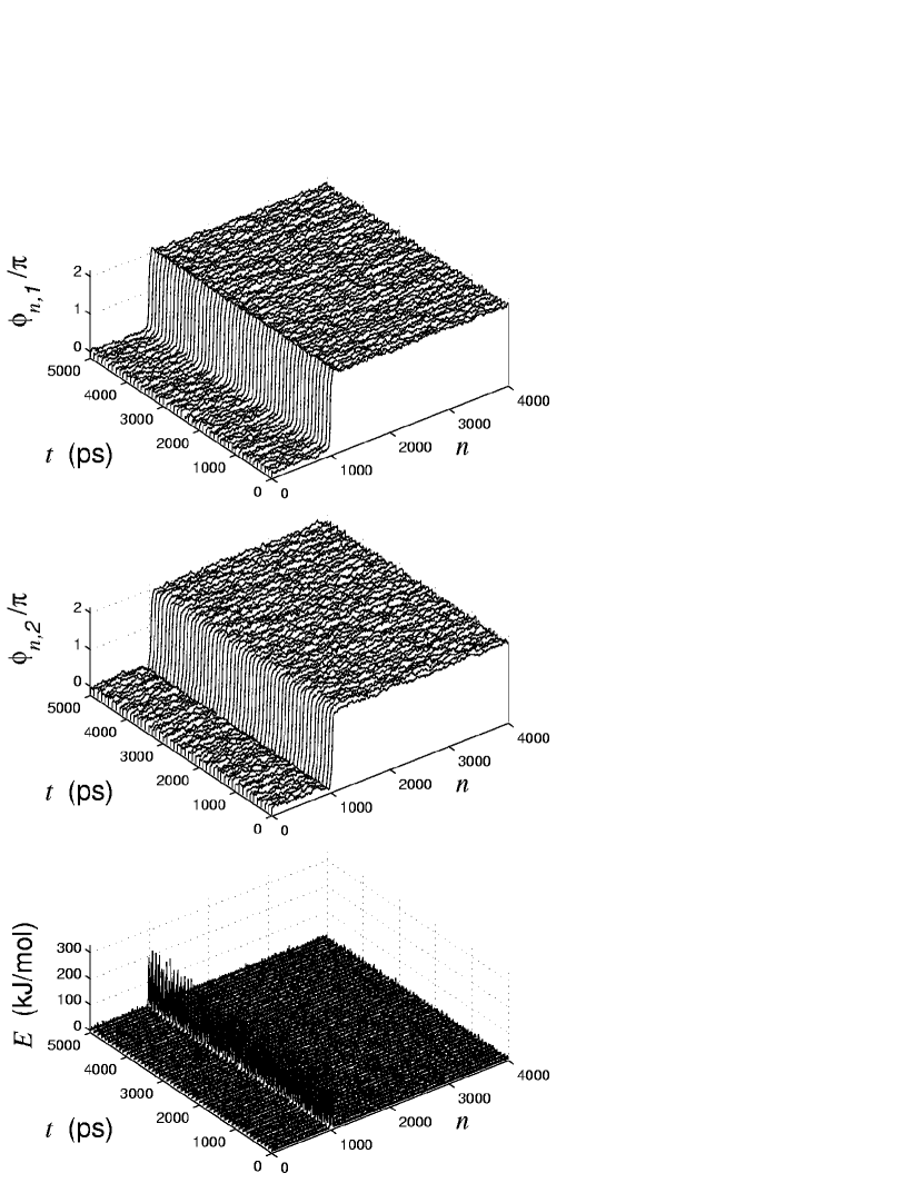
Figure 13: Stability of topological soliton (q$=(1,1)_{l}$, $s=0.5$) in the thermalized homogeneous AT chain ($T=300$K, $t_{r}=1$ ps). Dependence of the distribution of angular displacements $\varphi_{n,1}$, $\varphi_{n,2}$ and energy $E_{n}$ along the chain on time $t$ is shown ($K=0.234$ N/m).

Let us check stability of topological soliton with respect to thermal oscillations of the chain. For the purpose, let us consider homogeneous periodical AT chain consisting of $N=4000$ base pairs at the temperature $T=300$K. Let us integrate system (19) with the initial condition corresponding to topological soliton $(s=0.5)$ with center placed in the point $n=N/4$. Numerical integration shows stability of solitons at all values of the charge and at both values of the transverse rigidity $K=0.234$ N/m and $K=0.8714$ N/m. The viscosity of the environment leads to quick stop of the soliton, and after that all time it remains immovable. Soliton remains stable with respect to thermal oscillations during the all time of numerical integration $t=5\times 10^{3}$ ps (Fig. 13).

Let us note that in contrast to the models of phi-4 and of sine-Gordon the stability of solitons in the DNA model has not topological nature. Solitons can be destroyed. To show this, it is enough to suggest that the soliton width is equal to one base pair (soliton of that type is equivalent to the ground state of the chain). Here the stability is associated with energetic factors. From Fig. 13 it is well seen that in the region of localization of the soliton, the density of the energy is equal to $E_{n}\gg k_{B}T$.

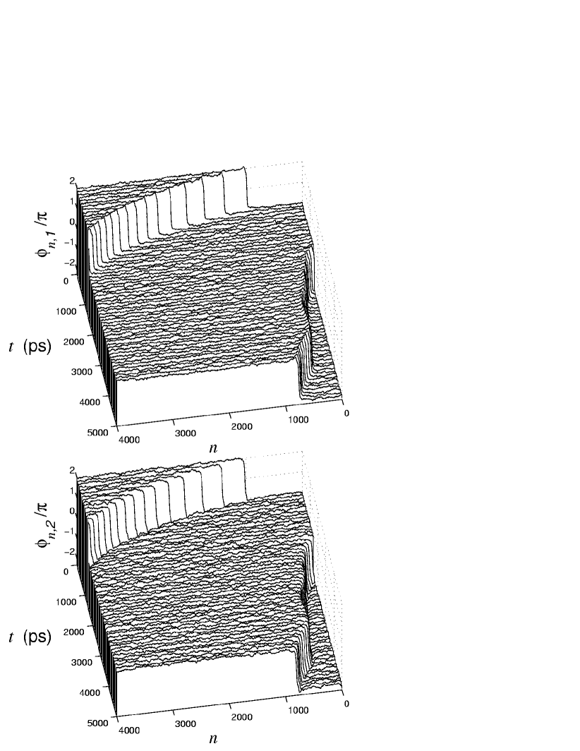
Figure 14: The braking of topological soliton (charge q$=(1,1)_{l}$, initial velocity $s=0.5$) in the thermalized cyclic homogeneous AT chain ($T=300$K, $K=0.234$ N/m and $t_{r}=1000$ps).

Soliton path length in the thermalized homogeneous chain ($T=300$K) depends on the value of relaxation time $t_{r}$ (on the viscosity of the surrounding of the molecule). At strong viscosity $t_{r}=1$ ps soliton has time to pass only 7 chain links till full stop. Then it remains immovable all the time (Fig. 13). When the viscosity is lower $t_{r}=10$ ps soliton has time to pass 41 links, and when $t_{r}=100$ ps – 480 links. The braking of soliton at low viscosity ($t_{r}=1000$ ps) is shown in Fig. 14. Soliton passes more than 3000 chain links, and then it begins to move as a massive Brownian particle.

The braking of soliton in the homogeneous chain is conditioned only by viscosity. When the viscosity is absent ($t_{r}=\infty$) soliton is moving along thermalized chain with constant velocity (Fig. 15).Thetmal phonons by themselves do not influence the soliton dynamics.

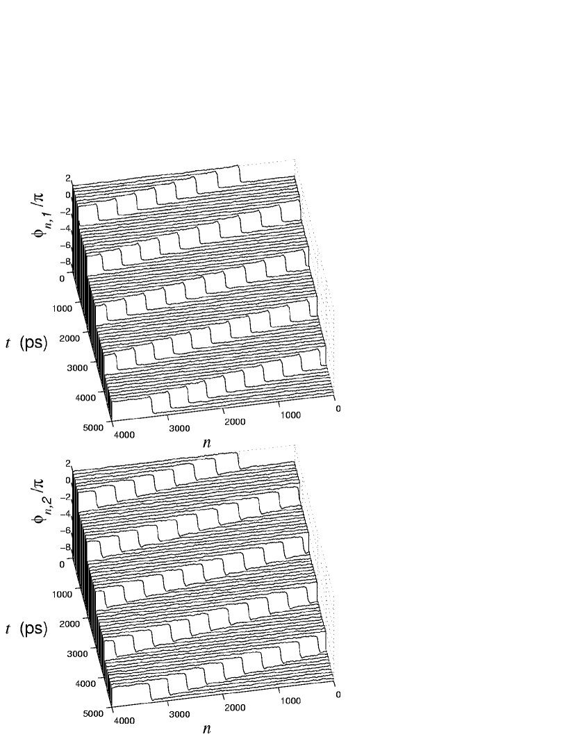
Figure 15: Movement of topological soliton (charge q$=(1,1)_{l}$, initial velocity $s=0.5$) in the thermalized cyclic homogeneous AT chain ($T=300$K, $K=0.234$ N/m and $t_{r}=\infty$).

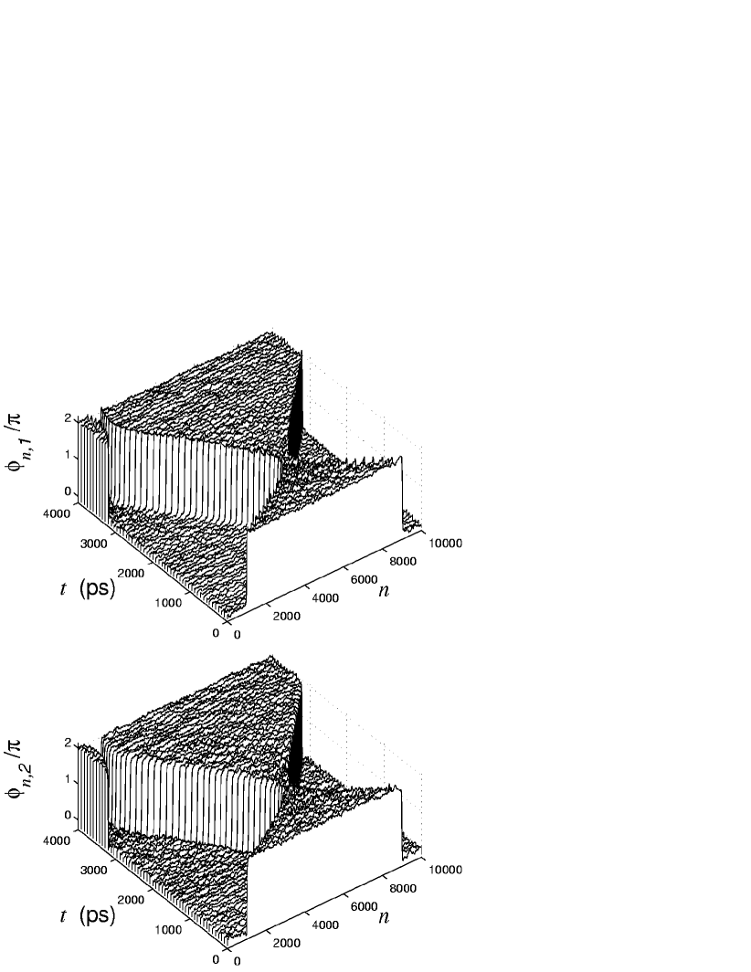
Figure 16: Reflection of topological solitons with different charges and polarities (${\bf q}_{1}=(1,1)_{l}$, ${\bf q}_{2}=(-1,1)_{r}$, $s_{1}=-s_{2}=0.5$) in the thermalized $(T=300$K) cyclic homogeneous AT chain ($K=0.234$ N/m, $t_{r}=\infty$).

Let us note that topological soliton can move along the DNA chain in the presence of viscosity too. To organize the propagation it is necessary to select in a special way the sequence of bases. If concentration of AT base pairs monotonically increases, inclined potential $E(n)$ is formed. The energy overfall can reach 1116 kJ/mol at $K=0.234$ N/m and 1894 kJ/mol at $K=0.8714$ N/m. Soliton will propagate along the relief inclination as a Brownian particle moving in the viscous media under the action of external constant force.

Thermal phonons substantially influence the interaction of solitons. In the work p42 , it was shown that topological solitons of the model $\phi$–4, can interact with one another through thermal phonons. This interaction comes to repulsion of the solitons. As a result, in the thermalized chain the interaction of the solitons of different charges substantially changes. At a long distance they will repulse. To model this phenomenon, let us consider collision of solitons with different charges and polarities in the thermalized cyclic AT chain $({\bf q}_{1}=(1,1)_{l}$, ${\bf q}_{2}=(-1,-1)_{r}$, $s_{1}=-s_{2}=0.5$). In the nonthermalized chain ($T=0$K), the solitons attract one another, and the collision leads to their recombination. In the thermalized cyclic chain ($T=300$K), their collision always leads to reflection (Fig. 16). This behavior can be explained by compression of phonons gas between solitons when they are drawing together. The compression leads to the repulsion of solitons, which increases as far as they are drawing together. In the chain with free ends, the compression of the phonon gas leads to long range repulsion of the solitons from the ends of the chain.

Thus, topological solitons of the DNA chains are stable with respect to thermal oscillations. Interaction with thermal phonons does not lead to destruction or to the braking of the soliton, it leads only to changing the interaction between the solitons. In the thermalized chain, long range repulsion between solitons is appeared.

IX Conclusion

Investigation carried out in this paper shows that three types of topological solitons which imitate localized states with open base pairs, can exist in the considered asymmetrical model of the DNA double chain. It was shown that the solitons can move along the macromolecule with constant velocity which is smaller than the sound velocity. In the inhomogeneous chain, the character of the soliton movement depends on the sequence of base pairs in the molecule. In the chain with random inhomogeneous sequence, solitons can move at a distance no more than several hundreds of base pairs. The results of numerical investigations show that the solitons are stable with respect to thermal oscillations. Interaction of the solitons with thermal phonons of the macromolecule does not lead to destruction or to the braking of the solitons. And only the character of their interactions changes. The drawing of the solitons together leads to their repulsion, which is explained by compression of phonon gas between them.

All these results point out that topological solitons of this type can be used to explain the long range effects in the DNA macromolecule.

References

- (1) H. Fritzshe, Comm. Mol. Biophys. 1, 325 (1982).
- (2) J. W. Keepers, Th. L. James, J. Am. Chem. Soc. 104, 929 (1982).
- (3) W. R. McClure, Ann. Rev. Biochem. 54, 171 (1982).
- (4) J. A. McCommon, S. C. Harvey, Dynamics of proteins and nucleic acids, Cambridge: Cambridge University Press, 1987.
- (5) L. V. Yakushevich, Quart. Rev. Biophys. 26, 201 (1993).
- (6) L. V. Yakushevich, V. M. Komarov, Mathematics. Computer. Education (in Russian), 5, 310 (1998).
- (7) S. M. Lindsay, J. W. Powell, E. W. Prohofsky, K. V. Devi-Prasad, Lattice modes? Soft modes and local modes in double helical DNA. in Structure and Dynamics of Nucleic Acids, Proteins and Membranes. Clementi E., Corongiu G., Sarma M. H., Sarma R. H., Eds. – New York: Adenine Press, 1984. – P. 531–551.
- (8) J. M. Eyster, W. Prohofsky, Biopolymers 13, 2505 (1974).
- (9) W. N. Mei, M. Kohli, E. W. Prohofskii, L. L. Van Zandt, Biopolymers 20, 833 (1981).
- (10) J. M. Eyster, W. Prohofsky, Biopolymers 16, 965, (1977).
- (11) M. Levitt, Cold Spring Harb. Symp. Quant. Biol. 47, 251 (1983).
- (12) B. Tidor, K. I. Irikura, B. R. Brooks, M. Karplus, J. Biomol. Struct. Dyn. 1, 231 (1983).
- (13) D. Flatters, R. Lavery, Biophys. J. 75, 372 (1998).
- (14) S. W. Englander, N. R. Kallenbach, A. J. Heeger, J. A. Krumhansl, A. Litwin, Proc. Natl. Acad. Sci. USA 77, 7222 (1980).
- (15) S. Yomosa, Phys. Rev. A. 27, 2120 (1983).
- (16) S. Takeno, S. Homma, Prog. Theor. Phys. 70, 308 (1983).
- (17) J. A. Krumhansl, D. M. Alexander, Nonlinear dynamics and conformational excitations in biomolecular materials. in Structure and dynamics: nucleic acids and proteins. Clementi E, Sarma R H., Eds. - New York: Adenine Press, 1983. – P. 61–80.
- (18) V. K. Fedyanin, I. Gochev, V. Lisy, Stud. biophys. 116, 59 (1986).
- (19) L. V. Yakushevich, Phys. Lett. A. 136, 413 (1989).
- (20) Ch.- T. Zhang, Phys. Rev. A. 35, 886 (1987).
- (21) V. Muto, P.S. Lomdahl and P. L. Christiannsen, Phys. Rev. A 42, 7452 (1990).
- (22) M. Peyrard, A. R. Bishop, Phys. Rev. Lett. 62, 2755 (1989).
- (23) S. N. Volkov, J. Theor. Biol. 143, 485 (1990).
- (24) G. Gaeta, Phys. Lett. A. 143, 227 (1990).
- (25) M. Salerno, Phys. Rev. A. 44, 5292 (1991).
- (26) L. L. Van Zandt, Phys. Rev. A. 40, 6134 (1989).
- (27) M. Techera, L. L. Daemen, E.W. Prohofsky, Phys. Rev. A. 41, 4543 (1990).
- (28) M. Barbi, S. Cocco, M. Peyrard, S. Ruffo, J. Biol. Phys. 24, 97 (1999).
- (29) M. Barbi, S. Cocco, M. Peyrard, Phys. Let. A. 253, 358 (1999).
- (30) A. Campa, Phys. Rev. E. 63, 021901 (2001).
- (31) P. L. Christiansen, A. V. Savin, A. V. Zolotaryuk, J. Comp. Phys. 134, 108 (1997).
- (32) P. L. Christiansen, A. V. Zolotaryuk, A. V. Savin, Phys. Rev. E 56, 877 (1997).
- (33) L. I. Manevitch, A. V. Savin, Phys. Rev. E 55, 4713 (1997).
- (34) A. V. Savin, L. I. Manevitch, Phys. Rev. B 58, 11386 (1998).
- (35) A. V. Savin, L. I. Manevitch, Phys. Rev. E 61, 7065 (2000).
- (36) A. V. Savin, L. I. Manevitch, Phys. Rev. B 63, 224303 (2001).
- (37) M. V. Volkenstein, Biophysics. – Published by Amer. Inst. of Physics, 1975.
- (38) M. B. Hakim, S. M. Lindsay, J. Powell, Biopolymers 23, 1185 (1984).
- (39) S. M. Lindsay, J. Powell, Light scattering of lattice vibrations of DNA. in: Structure and Dynamics: Nucleic Acids and Proteins. Clementi E., Sarma R.H., Eds. – New York: Adenine Press, 1983. – P. 241–259.
- (40) T. Weidlich, S. M. Lindsay, S. A. Lee, N. - J. Tao, G. D. Lewen, W. L. Peticolas, G. A. Thomas, A. Rupprecht, J. Phys. Chem. 92, 3315 (1988).
- (41) J. W. Powell, G. S. Edwards, L. Genzel, F. Kremer, A. Wittlin, W. Kubasek, W. Peticolas, Phys. Rev. A. bf 35, 3929 (1987).
- (42) O. P. Kolbysheva, A. F. Sagdeev, JETP 100, 1262 (1991).