Neutral Plasma Oscillations at Zero Temperature

Abstract

We use cold plasma theory to calculate the response of an ultracold neutral plasma to an applied rf field. The free oscillation of the system has a continuous spectrum and an associated damped quasimode. We show that this quasimode dominates the driven response. We use this model to simulate plasma oscillations in an expanding ultracold neutral plasma, providing insights into the assumptions used to interpret experimental data [Phys. Rev. Lett. 85, 318 (2000)].

Recent experimental rolston98 ; killian99 ; kulin00 ; robinson00 ; killian01 ; dutta01 and theoretical work cote00 ; greene00 ; tkachev01 ; hahn01 ; robicheaux02 ; mazevet02 ; kuzmin02 has studied the formation and evolution of ultracold plasmas. In the laboratory, cold plasmas are created either by directly photo-ionizing laser-cooled atoms, or by exciting the atoms to high-lying Rydberg states that spontaneously ionize. A fraction of the electrons escape the plasma and the resulting electric field drives the ion expansion. Models of the expansion suggest that the density profile in the plasma is approximately Gaussian, and that it expands in a self-similar manner. It can be expressed as

$$n(r,t)={{n_{0}\sigma_{0}^{3}}\over{\sigma^{3}}}\exp[-r^{2}/2\sigma^{2}]~{},$$ (1)

where $\sigma=\sqrt{\sigma_{0}^{2}+v^{2}t^{2}}$ is the time-dependent width of the distribution, $v$ is the asymptotic expansion velocity, and $t$ is time.

The experimental justification of this density profile for the case of an expanding plasma is based on the plasma’s response to a spatially uniform applied rf field. In those experiments, Xe atoms initially cooled to $\sim 10\mu$K were ionized by a dye laser. The initial electron energy ($E_{e}/k_{B}$) ranged from a few to 1000 K, and the initial electron density ranged from $0.2$ to $2.5\times 10^{9}$ cm^-3. The plasmas were nearly charge-neutral, and at electron energies above 70 K, the kinetic energy of the electrons allowed significant loss. The resulting net positive charge in the cloud drove the plasma expansion.

As the plasma expanded and its density decreased, the applied rf field pumped energy into the plasma. The heating was assumed to be largest where the applied rf frequency matched the local plasma frequency. Because of collisions in the plasma, the local heating presumably raised the overall plasma temperature, and a small number of the more weakly-bound electrons were ejected. The experiment measured the rate at which electrons were ejected from the expanding plasma as a function of time for a fixed applied rf frequency. This signal was presumed to be proportional to the rate at which the rf field heats the plasma, and was a measure of the weighted time-dependent density profile.

The peak of this signal was interpreted to correspond to the “average” density of the plasma,

$$\bar{n}(t)=2^{-3/2}n(0,t)={{n_{0}\>\sigma_{0}^{3}}\over{\left[2\left(\sigma_{0}^{2}+v^{2}t^{2}\right)\right]^{3/2}}}$$ (2)

with $v$ a constant. This density was experimentally determined by setting the applied frequency $\omega$ equal to the average plasma frequency, $\omega_{p}$, and using the relation $\bar{\omega}_{p}=\sqrt{q^{2}\bar{n}(t)/m_{e}\epsilon_{0}}$, where $q$ is the electron charge, $m_{e}$ is the electron mass, and $\epsilon_{0}$ is the permittivity of free space. The derived density, $\bar{n}$, is time dependent. For a different applied rf frequency $\omega$, the signal peaks at a different time. A least-squares fit of $\bar{n}(t)$ to Eq. (2) gives the initial density $n_{0}$ and the expansion velocity $v$.

In this paper, we examine the validity of the assumptions used in this interpretation by presenting the response of the system predicted by cold plasma theory. This theory is good for plasmas in which $(\lambda_{D}/\sigma)^{2}\ll 1$, where $\lambda_{D}$ is the Debye length. In the experiments we are simulating, $(\lambda_{D}/\sigma)^{2}\approx 10^{-3}-10^{-1}$, making cold plasma theory a good way to model the collective response of the system.

We consider spherically symmetric charge-neutral Gaussian distributions of cold ions and electrons to which an rf-electric field in the $z$-direction is applied. The ions are taken as fixed on the time-scale of the rf oscillation. The fluid equations describing the electrons are

$${{\partial n}\over{\partial t}}+\nabla\cdot\left(n\vec{v}\right)=0$$ (3)

$$\nabla^{2}\phi=-q\left(n-n_{i}\right)/\epsilon_{0}$$ (4)

$$m\left({{\partial\vec{v}}\over{\partial t}}+\vec{v}\cdot\nabla\vec{v}\right)=q\vec{E}-\gamma m\vec{v}.$$ (5)

In these equations $n=n(r,t)$ is the electron density, $n_{i}=n_{i}(r)$ is the ion density (assumed to be fixed in time), $\vec{v}=\vec{v}(\vec{r},t)$ is the electron velocity, $\vec{E}=\vec{E}(\vec{r},t)$ is the total electric field (the sum of the external field and that generated by the plasma response), and $\gamma$ is a phenomenological damping rate. Some effects of finite temperature, such as electron-electron collisions and electron-ion collisions, are approximated by the the parameter $\gamma$.

In the experiment by Kulin et al. kulin00 , the applied $\vec{E}$ was uniform in space and oscillating in the $\hat{z}$-direction. Assuming that this applied field is small, the fluid equations can be linearized by assuming that the density and the potential are of the form $n(r,\theta,t)=n^{(0)}(r)+\delta n(r)\cos{\theta}e^{-i\omega t}$, where $n^{(0)}(r)$ is the equilibrium electron density, and $\phi(r,\theta,t)=\delta\phi(r)\cos{\theta}e^{-i\omega t}$ (spherical harmonics with $\ell=1$). After some algebra to linearize the fluid Equations (3)-(5), the potential produced by the electrons is given by the expression

$${\cal{L}}\delta\phi-{{\left[{{d}\over{dr}}\omega_{p}^{2}(r)\right]{{\partial\delta\phi}\over{\partial r}}}\over{\omega^{2}-\omega_{p}^{2}(r)+i\omega\gamma}}=-{{\left[{{d}\over{dr}}\omega_{p}^{2}(r)\right]E_{0}}\over{\omega^{2}-\omega_{p}^{2}(r)+i\omega\gamma}}$$ (6)

where the operator $\cal{L}$ is defined as

$${{d^{2}}\over{dr^{2}}}+{{2}\over{r}}{{d}\over{dr}}-{{2}\over{r^{2}}}$$ (7)

and where $\omega_{p}(r)=\sqrt{q^{2}n^{(0)}(r)/m_{e}\epsilon_{0}}$ is the plasma frequency. The boundary conditions are that $\delta\phi(0)=0$ and that at infinity the field is that of a dipole, $\delta\phi(r)\propto 1/r^{2}$.

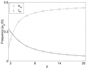
Figure 1: Quasimode frequency, $\omega_{m}$ ($\circ$), and damping rate, $\gamma_{m}$ ($\diamond$), for density profiles given by Eq. (8). For $p=2$, the distribution is Gaussian. As $p$ increases, the distribution approaches a “top-hat,” the quasimode frequency increases, and the quasimode damping decreases (see text).

Because this is a driven system, we first look for normal modes. Notice, however, that with $E_{0}=0$ and $\gamma=0$ (undamped free response) this mode equation has a continuous spectrum, similar to the diocotron mode equation in non-neutral plasmasschecter99a ; spencer97 ; corngold95 ; briggs70 ; case60 ; kelvin80 . And, as with the diocotron mode, this equation also has a damped quasimode. Following Ref. spencer97 , Eq. (6) can be solved along a contour in the complex $r$-plane to uncover this damped quasimode. Figure 1 shows the frequency and damping rate of this quasimode for a sequence of density profiles of the form

$$n(r)=n_{0}e^{-r^{p}/2\sigma^{p}}$$ (8)

The real and imaginary parts of the quasimode frequency are well approximated by the simple formulas $\omega_{m}/\omega_{p}(0)=1/\sqrt{3}-0.668/p-0.102/p^{2}$ and $\gamma_{m}/\omega_{p}(0)=1.077/p-0.959/p^{2}$.

Note that the Gaussian ($p=2$) quasimode is heavily damped and that as $p$ becomes large (making the density profile approach a step-profile) the damping rate goes to zero and the frequency approaches $\omega_{m}=\omega_{p}(0)/\sqrt{3}$.

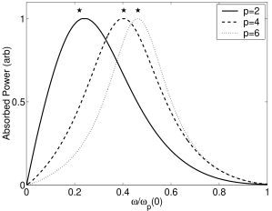
Figure 2: Power absorbed by the (non-expanding) plasma as a function applied frequency. The solid line shows the absorbed power for a Gaussian density profile, $p=2$ in Eq. (8). Also shown is the absorbed power for super-Gaussian profiles, with $p=4,6$. The mode damping decreases with increasing $p$. These plots are generated with $\gamma/\omega_{p}^{(0)}=0.01$. For larger values of $\gamma$, these curves are somewhat broader and shifted to slightly higher $\omega$.

The quasimode dominates the free response of a system with a continuous spectrum schecter00 ; schecter99 . It also strongly influences the driven response, as can be seen in Fig. 2. This figure shows the rate at which a plasma absorbs power from an applied rf field as a function of the frequency of that field. To calculate this power, we note that the total electric field (the applied field plus the plasma response) is given by

$$\vec{E}(r,t)=\left(\hat{z}E_{0}\cos\theta-\nabla\delta\phi\right)e^{-i\omega t}.$$ (9)

By using the linearized Eq. (5) to compute the current density $\vec{J}=qn\vec{v}$ in the plasma, the power density can be written as

$$\left<P\right>={{1}\over{2}}Re\left(\vec{E}\cdot\vec{J}^{*}\right)={{\epsilon_{0}}\over{2}}\left|\vec{E}\right|^{2}{{\omega_{p}^{2}(r)\gamma}\over{\omega^{2}+\gamma^{2}}}.$$ (10)

The influence of the quasimode on the absorbed power can be seen by integrating this power density over all space for various values of the driving frequency $\omega$. Although strongly damped, the quasimode still influences how the plasma responds to the rf field. Figure 2 shows the calculated power absorbed by the plasma as a function of the applied rf frequency for a non-expanding plasma. In each case the peak of the absorbed power occurs near the frequency of the quasimode. Notice that these resonances occur at quite small values of the density, rather than in the body of the density distribution as assumed by Kulin, et al. The experiment used $\omega/\omega_{p}(0)=0.6$

We now use these cold driven solutions of Eq. (6) to simulate the plasma expansion experiment. In order to do this, we need an expression for the electron density, $n(r,t)$ and the phenomenological damping rate $\gamma$. For both of these we use the model of Robicheaux and Hanson robicheaux02 . They simulated an expanding ultracold neutral plasma to study three-body recombination and electron heating. An important result of their paper is that the electron temperature scales with density as $T_{e}\propto n^{-1/3}$, which makes the Coulomb logarithm ($\ln\Lambda$) constant. We use this result in our simulation of the collective response of the plasma to an applied field. It is likely that the phenomenological damping rate, $\gamma$, is proportional to the electron collision rate, $\nu$. The scaled collision rate in the plasma is $\nu/\omega_{p}\propto\sqrt{n/T^{3}}\ln\Lambda$, which is constant in this temperature scaling. For typical experimental parameters, this gives $\gamma/\omega_{p}(0)\approx 1/100$. Another important result from the work of Robicheaux and Hanson is that most of the ions in the plasma experience an electric field linearly proportional to $r$. Given the known initial conditions in the plasma, this leads directly to the result that the plasma density is Gaussian, and that it expands in a self-similar manner described by Eq. (1) note01 .

We simulate the plasma expansion experiment as follows. The plasma expansion velocity ($v$), the rf frequency ($\omega$) and rf amplitude ($E_{0}$) are held constant. At a particular time $t$, we insert the density from Eq. (1) into Eq. (6) to find the potential $\delta\phi$ and the total electric field [Eq. (9)]. We integrate the power density [Eq. (10)] over the spatial coordinates to get the plasma heating rate at that time. We increment time and repeat the heating rate calculation to generate one of the time-sweeps shown in Fig. 3(a). Repeating these calculations for a range of applied field frequencies generates all of the time sweeps shown in the figure.

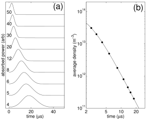
Figure 3: (a) Calculated plasma heating rate. The applied frequencies $\omega/2\pi$ in MHz are shown to the left of each trace. The traces are offset vertically for clarity. The plasma conditions are $n_{0}=10^{15}$ m^-3, $v=100$ m/s, $\sigma_{0}=220\;\mu$m, and $\gamma/\omega_{p}(0)=0.01$. (b) Average plasma density as a function of time. The circles ($\bullet$) are taken from the data in (a). The applied frequency is converted to a density, $\bar{n}(t)$, with $t$ given by the peak of the signal (see text). The solid line is a fit of these points to Eq. (2). The fitted density is $\bar{n}=1.1\times 10^{14}$ m^-3 or $n_{0}=3.1\times 10^{14}$ m^-3, about a factor of $3$ too low. The fitted expansion velocity is $v=100$ m/s.

We convert the time sweeps in Fig. 3(a) into average density determinations. At the peak of each time sweep we set the applied frequency $\omega$ equal to the average plasma frequency $\bar{\omega}_{p}=\sqrt{q^{2}\bar{n}/m_{e}\epsilon_{0}}$ to calculate the average density $\bar{n}$, as was done in the experiment kulin00 . With this conversion from frequency to density, the simulated average density $\bar{n}(t)$ is plotted in Fig. 3(b). The data is fit to Eq. (2) using a least-squares method to extract the initial central density, $n_{0}$, and expansion velocity $v$.

The shapes of the calculated plasma heating rates shown in Fig. 3(a) match the experimental ones from Reference kulin00 , and the fit of $\bar{n}(t)$ in Fig. 3(b) to Eq. (2) is excellent note03 . The expansion velocity extracted from the fit exactly matches the known velocity that we put into the simulation, independent of the value of the scaled damping rate $\gamma/\omega_{p}(0)$. If the Robicheaux and Hanson temperature scaling is correct, the plasma response to the rf field accurately reproduces the true asymptotic expansion velocity. However, different temperature scalings make the fit worse. If instead of using $T\propto n^{1/3}$ in determining $\gamma$, we use $T\propto n^{2/3}$, the fitted velocity increases by roughly a factor of two, depends on $\gamma/\omega_{p}(0)$, the extracted $\bar{n}(t)$ does not follow Eq. (2), and the simulation does not fit the experiment.

The initial central density $n_{0}$ extracted from the fit of $\bar{n}(t)$ to Eq. (2) is quite sensitive to the scaled damping factor, $\gamma/\omega_{p}(0)$. It scales approximately as $e^{2\gamma/\omega_{p}(0)}$. It also depends on the particular temperature scaling used in the simulation, and can vary by orders of magnitude. For the Robicheaux and Hanson temperature scaling and with $\gamma/\omega_{p}(0)=0.01$, the fitted central density underestimates the known central density in our simulation by a factor of three.

Cold plasma theory only addresses the collective behavior of the system. Another effect that might be involved in the resonant behavior seen in the experiment is that the electron motion in the plasma resonates with the driving field. Robicheaux and Hanson estimate that in the bulk of the plasma the potential satisifes $q\phi/k_{B}T=r^{2}/2\sigma^{2}$. This means that most of the particles are in an isotropic harmonic oscillator well with natural frequency $\omega_{0}=\omega_{p}(0)\lambda_{D}(0)/\sigma$, where $\lambda_{D}(0)$ is the Debye length at the center of the cloud. If the peaks in the experiment were due to particle resonance at $\omega=\omega_{0}$ in the expanding plasma, the experiment does not indicate a uniform expansion note02 .

However, in experiments where $\lambda_{D}(0)\ll\sigma$, such as in the present simulations, we would expect collective effects like the quasimode, to dominate over individual particle effects like a resonance at $\omega=\omega_{0}$. But even though collective effects should dominate these plasmas, particle resonance can play a role, as it does in the case of electron Bernstein wave in magnetized plasmas krall73 . Calculating this effect requires a kinetic theory treatment that is beyond the scope of this paper. But we note that even in kinetic theory the particle resonance will not be sharp because the well is not perfectly parabolic, causing the orbit frequency to vary with the energy and angular momentum. Averaging this resonance over the distribution function blurs its effect and makes the resonances at $\omega_{0}$, $2\omega_{0}$, etc. less pronounced.

It would be very helpful to have direct measurements of the ion density distribution, such as with optical detection. These measurements could provide benchmark data against which future simulations can be compared. Also, as mentioned previously, full kinetic simulations are probably required to address the particle orbit problem. Such measurements and simulations are currently underway in our laboratory.

In conclusion, we have used a simulation based on cold plasma theory to calculate the response of an ultracold plasma to an applied rf field. When $T\propto n^{1/3}$, the simulation accurately reproduces the experimental data of Kulin et al. kulin00 , providing an important consistency check of the model of Robicheaux and Hanson robicheaux02 .

The model confirms that the plasma response accurately reproduces the asymptotic velocity of an expanding plasma, and determines the initial plasma density to within a factor of two or three. The plasma response is dominated by the quasi-mode. Even though the mode is strongly damped, it shifts the plasma resonance to lower densities than otherwise expected from a local-density approximation.

This work is supported in part by grants from the Research Corporation and from the National Science Foundation under Grant No. PHY-9985027.

References

- (1) S. L. Rolston, S. D. Bergeson, S. Kulin, and C. Orzel, Bull. Am. Phys. Soc. 43, 1324 (1998).
- (2) T. C. Killian, S. Kulin, S. D. Bergeson, L. A. Orozco, C. Orzel, and S. L. Rolston, Phys. Rev. Lett. 83, 4776 (1999)
- (3) S. Kulin, T. C. Killian, S. D. Bergeson, and S. L. Rolston, Phys. Rev. Lett. 85 318 (2000).
- (4) M. P. Robinson, B. Laburthe Tolra, Michael W. Noel, T. F. Gallagher, and P. Pillet, Phys. Rev. Lett. 85, 4466 (2000)
- (5) T. C. Killian, M. J. Lim, S. Kulin, R. Dumke, S. D. Bergeson, and S. L. Rolston, Phy. Rev. Lett. 86, 3759 (2001)
- (6) S. K. Dutta, D. Feldbaum, A. Walz-Flannigan, J. R. Guest, and G. Raithel, Phys. Rev. Lett. 86, 3993 (2001)
- (7) R. Côté and A. Dalgarno, Phys. Rev. A 62, 012709 (2000)
- (8) C. H. Greene, A. S. Dickinson, and H. R. Sadeghpour, Phys. Rev. Lett. 85, 2458 (2000)
- (9) A. N. Tkachev and S. I. Yakovlenko, JETP Let. 73, 66-68 (2001)
- (10) Y. Hahn, Phys. Rev. E 64, 046409 (2001)
- (11) F. Robicheaux and James D. Hanson, Phys. Rev. Lett. 88, 055002 (2002)
- (12) S. Mazevet, L. A. Collins, and J. D. Kress, Phys. Rev. Lett. 88, 055001 (2002)
- (13) S. G. Kuzmin and T. M. O’Neil, Phys. Rev. Lett. 88, 065003 (2002)
- (14) D. A. Schecter, D. H. E. Dubin, A. Cass, C. F. Driscoll, I. M. Lansky, and T. M. O’Neil, in Non-Neutral Plasma Physics III, edited by John J. Bollinger, et al., American Institute of Physics 1999).
- (15) R. L. Spencer and S. N. Rasband, Phys. Plasmas 4, 53 (1997).
- (16) R. J. Briggs, J. D. Daugherty, and R. H. Levy, Phys. Fluids 13, 421 (1970);
- (17) K. M. Case, Phys. Fluids 3, 143 (1960).
- (18) W. Kelvin, Nature 23, 45 (1880).
- (19) N. R. Corngold, Phys. Plasmas 2, 620 (1995).
- (20) D. A. Schecter, D. H. E. Dubin, A. C. Cass, C. F. Driscoll, I. M. Lansky, and T. M. O’Neil, Phys. Fluids 12 2397 (2000).
- (21) D. A. Schecter, D. H. E. Dubin, A. C. Cass, C. F. Driscoll, I. M. Lansky, and T. M. O’Neil, AIP Conf. Proc. 498, 115 (1999).
- (22) In Reference robicheaux02 , the density is written as , where is the number of ions. The function is given by Eq. (2) in that paper, and can be solved analytically. For the given boundary conditions, it is , making their expression for density identical to Eq. (1) in this work.
- (23) The calculated plasma heating rates shown in Fig. 3(a) match the experimental rates when recombination can be neglected (K kulin00 ; killian01 ). Recombination depletes the low-temperature part of the electron distribution. This translates into experimentally measured heating rates that fall off more sharply than those shown in Fig. 3(a), measured average density functions that do not match Eq. 2, and expansion velocities greater than expected from the initial electron energy.
- (24) In the asymptotic limit where , the model of Robicheaux and Hanson predicts that the resonant frequency is given by . If the resonances in the experiment were given by this response, the density profile would have to be either distinctly non-Gaussian, or experience a complicated expansion in time.
- (25) N. A. Krall and A. W. Trivelpiece, Principles of Plasma Physics, (McGraw-Hill, New York, 1973).