Bound State Calculations for Three Atoms Without Explicit Partial Wave Decomposition

Abstract

A method to calculate the bound states of three-atoms without resorting to an explicit partial wave decomposition is presented. The differential form of the Faddeev equations in the total angular momentum representation is used for this purpose. The method utilizes Cartesian coordinates combined with the tensor-trick preconditioning for large linear systems and Arnoldi’s algorithm for eigenanalysis. As an example, we consider the He₃ system in which the interatomic force has a very strong repulsive core that makes the three-body calculations with standard methods tedious and cumbersome requiring the inclusion of a large number of partial waves. The results obtained compare favorably with other results in the field.

PACS numbers: 21.45.+v, 36.90.+f,02.70.Jn

I Introduction

In recent years the ⁴He trimer has been the center of several theoretical investigations (see, for example, Refs. Fedorov ; Roudnev ; Motoold and references therein). From all methods employed in these studies, the Faddeev equations method is perhaps the most attractive since it reduces the Schrödinger equation for three particles into a system of integral or differential equations which can be used to study bound states and scattering processes in a rigorous way.

The differential form of the Faddeev equations has been proposed long ago by Noyes and Fiedeldey Noyes . Since then, these equations have been used in bound states calculations in Nuclear and Coulomb systems GignLav ; MerkGignLav ; Friar ; KviHu ; YkFl – just to mention a few references. The derivation and discussion by Merkuriev of the asymptotic boundary condition of the differential Faddeev equations (DFE) Merkuriev , paved the way to use the DFE not only in bound-state calculations but in investigations of scattering processes as well. For atomic systems, however, some peculiarities of the inter-atomic interactions resulted in a limited use of DFE in both bound and scattering calculations.

One of the peculiarities is that the interaction among atoms often contains very strong repulsion at short distances which is difficult to handle numerically. In addition, it generates strong short range correlations implying that in atomic systems one should take into account many partial waves in order to achieve convergence. These problems can hardly be solved by using the computational power of modern computers and requires instead the development of appropriate numerical techniques.

One such technique is the so-called tensor-trick proposed by the Groningen group Groning ; Groning1 . Application of the method in Nuclear and Coulomb systems showed that high accuracy calculations can be made using low computer power. Another method is that of Cartesian coordinates applied for the first time in three body Faddeev calculations in Carbonell . The latter method is suitable in describing the long-range behavior of weakly three-body bound states correctly. This feature is crucial in calculating excited states close to the two-body threshold. Yet another proposed method of solving the three-body problem is that of Ref. Kvits in which no explicit partial wave decomposition is required and only the total angular momentum of the system is used. Within this total angular momentum representation method the Faddeev operator has a very simple form that allows the construction of effective numerical schemes.

In the present work we have combined the aforementioned methods and, moreover, we propose a new approach to overcome the difficulties arising from the short range repulsion. We applied the overall procedure in bound state calculations of the He₃ system using various potentials and compare our results with other results previously obtained by various groups.

In Sec. II we describe the equations to be solved and formulate the appropriate boundary conditions. In Sec. III the numerical method is presented. Our results are given in Sec. IV while our conclusion are summarized in Sec. V. Some technical details for the field practitioners are shifted in the appendix.

II Formalism

When considering a three-body system it is convenient to denote the two-body subsystems by $\alpha$, $\beta$ and $\gamma$ and introduce Jacobi coordinates which in the configuration space are defined by

$$\begin{array}[]{rcl}\cr{\bf x}_{\alpha}&=&\displaystyle\left(\frac{2m_{\beta}m_{\gamma}}{m_{\beta}+m_{\gamma}}\right)^{1/2}({\bf r}_{\beta}-{\bf r}_{\gamma})\cr{\bf y}_{\alpha}&=&\displaystyle\left(\frac{2m_{\alpha}(m_{\beta}+m_{\gamma})}{m_{\alpha}+m_{\beta}+m_{\gamma}}\right)\left({\bf r}_{\alpha}-\displaystyle\frac{m_{\beta}{\bf r}_{\beta}+m_{\gamma}{\bf r}_{\gamma}}{m_{\beta}+m_{\gamma}}\right)\end{array}$$ (1)

The coordinates corresponding to other pairs can be obtained by cyclic permutations of the subscripts $\alpha$, $\beta$, and $\gamma$, their relation being

$$\left(\matrix{{\bf x}_{\beta}\cr{\bf y}_{\beta}}\right)=\left(\matrix{S^{11}_{\beta\alpha}&S^{12}_{\beta\alpha}\cr S^{21}_{\beta\alpha}&S^{22}_{\beta\alpha}\cr}\right)\left(\matrix{{\bf x}_{\alpha}\cr{\bf y}_{\alpha}}\right)\,$$ (2)

where $S^{ij}_{\beta\alpha}$ are coefficients which depend on the masses of the particles MerkFadd . For identical particles these coefficients are

$$S^{11}_{\beta\alpha}=S^{22}_{\beta\alpha}=\frac{1}{2}\,,\qquad S^{12}_{\beta\alpha}=-S^{21}_{\beta\alpha}=\frac{\sqrt{3}}{2}$$

We assume that the Hamiltonian of the system involves only two-body interactions

$$H=H_{0}+\sum_{i}V_{i}({\bf x}_{i})\,,$$ (3)

where $H_{0}=-\Delta_{x}-\Delta_{y}$ is the Hamiltonian of three free particles and $V_{i}({\bf x}_{i})$ are the two-body potentials.

The wave function $\Psi$ of the system can be expressed in terms of the three Faddeev components $\Phi_{i}$

$$\Psi({\bf x},{\bf y})=\sum_{i}\Phi_{i}({\bf x}_{i},{\bf y}_{i})\,$$ (4)

satisfying the Faddeev equations

$$(-\Delta_{x}-\Delta_{y}+V_{i}({\bf x}_{i})-E)\Phi_{i}({\bf x}_{i},{\bf y}_{i})=-V_{i}({\bf x}_{i})\sum_{j\neq i}\Phi_{j}({\bf x}_{j},{\bf y}_{j})$$ (5)

where $E$ is the energy of the system. In what follows we shall restrict ourselves, without loss of generality, to three identical bosons which is the case under consideration. In such a case the Faddeev components have the same functional form in their own coordinates and thus the system (5) is reduced to one equation only

$$(H_{0}+V-E)\Phi=-V(C^{+}+C^{-})\Phi\ .$$ (6)

In this equation $H_{0}=-\Delta_{x}-\Delta_{y}$, $C^{+}$ and $C^{-}$ are the cyclic and anticyclic permutation operators respectively, $\Phi$ is one of the Faddeev components $\Phi_{i}$ written in its own coordinates.

The potential energy of the system is invariant with respect to rotations. This makes it possible to separate out the degrees of freedom corresponding to rotations of the system. This can be achieved by expanding the Faddeev component $\Phi$ in terms of eigenfunctions of the total angular momentum, i.e. Wigner functions $D_{mn}^{L}(g)$ Kvits ,

$$\Phi({\bf x},{\bf y})=\sum_{L,m,n}\frac{\phi^{Lmn}(x,y,z)}{xy}\,D_{mn}^{L}(g)\,.$$ (7)

Here $g\in SO(3)$ are the coordinates describing collective angular motion of the system and $\phi^{Lmn}(x,y,z)$ are the projections of the Faddeev component in subspaces with fixed angular momentum. The components of the projections depend on the intrinsic coordinates

$$x=|{\bf x}|,\quad y=|{\bf y}|,\quad z=\frac{({\bf x},{\bf y})}{xy},\qquad x,y\in[0,\infty),\ \ z\in(-1,1)$$ (8)

which describe the intrinsic state of the cluster. Since we can fix the total angular momentum $L$ of the system, the corresponding projection of the free Hamiltonian can be written as

$$H_{0}^{L}=D^{L}(g^{-1})xyH_{0}\frac{1}{xy}D^{L}(g)$$ (9)

where $D^{L}(g)$ stands for a matrix constructed from the Wigner functions Kvits . In the case of zero total angular momentum the explicit expression for $H^{0}_{0}$ reads

$$H^{0}_{0}=-\frac{\partial^{2}}{\partial x^{2}}-\frac{\partial^{2}}{\partial y^{2}}-(\frac{1}{x^{2}}+\frac{1}{y^{2}})\frac{\partial}{\partial z}(1-z^{2})\frac{\partial}{\partial z}\,.$$ (10)

The corresponding projection of Eq. (6) takes the form

$$(H^{0}_{0}+V(x)-E)\phi^{0}(x,y,z)=-V(x)P\phi^{0}(x,y,z)\,,$$ (11)

where

$$P\phi^{0}(x,y,z)\equiv xy(\frac{\phi^{0}(x^{+},y^{+},z^{+})}{x^{+}y^{+}}+\frac{\phi^{0}(x^{-},y^{-},z^{-}))}{x^{-}y^{-}})$$

and $x^{\pm}(x,y,z)$, $y^{\pm}(x,y,z)$, and $z^{\pm}(x,y,z)$ are

$$\begin{array}[]{rcl}\displaystyle x^{\pm}(x,y,z)&=&\displaystyle(\frac{1}{4}x^{2}+\frac{3}{4}y^{2}\mp\frac{\sqrt{3}}{2}xyz)^{1/2}\;,\\ y^{\pm}(x,y,z)&=&\displaystyle(\frac{3}{4}x^{2}+\frac{1}{4}y^{2}\pm\frac{\sqrt{3}}{2}xyz)^{1/2}\;,\\ z^{\pm}(x,y,z)&=&\displaystyle\frac{\displaystyle\pm\frac{\sqrt{3}}{4}x^{2}\mp\frac{\sqrt{3}}{4}y^{2}-\displaystyle\frac{1}{2}xyz}{x^{\pm}(x,y,z)\,y^{\pm}(x,y,z)}\;.\end{array}$$ (12)

Assuming that in each two-body subsystem only one bound state exists, we can write the asymptotic boundary conditions for the Faddeev component $\phi^{0}$ as follows

$$\phi^{0}(x,y,z)\sim\,\varphi_{2}(x)\,{\rm e}^{-k_{y}y}+A(x/y,z)\,\frac{{\rm e}^{-k_{3}(x^{2}+y^{2})^{1/2}}}{(x^{2}+y^{2})^{1/4}}\,,$$ (13)

where $\varphi_{2}(x)$ denotes the wave function of the two-body bound state in the two-body subsystem, $k_{y}=\sqrt{E_{2}-E_{3}}$, $k_{3}=\sqrt{-E_{3}}$, $E_{2}$ is the two–body bound state energy, and $E_{3}$ the energy of the three-body system. The first term corresponds to virtual decay into a particle and a two-body bound system, usually denoted as 2+1, while the second term corresponds to a virtual decay with an amplitude $A(x/y,z)$ into three single particles denoted as 1+1+1. The term corresponding to the latter configuration decreases much faster than in the 2+1.

In the present work the term corresponding to 1+1+1 virtual decay is neglected and thus the asymptotic boundary conditions for the Faddeev component at sufficiently large distances $R_{x}$ and $R_{y}$ read

$$\left.\frac{\partial}{\partial x}\ln\phi^{0}(x,y,z)\right|_{x=R_{x}}=-k_{x}\equiv i\sqrt{E_{2}}\,,\qquad\left.\frac{\partial}{\partial y}\ln\phi^{0}(x,y,z)\right|_{y=R_{y}}=-k_{y}\,.$$ (14)

III Numerical Procedure

The first numerical calculation with the DFE were made by Laverne and Gignoux in the early seventies GignLav . Since then, many numerical methods were proposed. In the present work we shall employ: i) Quintique splines KviHu together with an orthogonal collocation deBoorSwartz procedure which allows us to construct a linear system of equations corresponding to Eq. (11). In this way the bound state problem can be transformed to a generalized eigenvalue problem. ii) The tensor-trick Groning to solve the eigenvalue problem using the restarting Arnoldi algorithm Saad .

Any regular solution of Eq. (11) fulfilling the boundary conditions (14) can be approximated by an expansion in terms of the basic functions (see Appendix A)

$$\phi^{0}(x,y,z)=\sum_{i}f_{i}B_{i}(x,y,z)$$ (15)

where $i$ stands for a multi–index $\{i_{x},i_{y},i_{z}\}$ and $B_{i}(x,y,z)=B_{i_{x}}(x)B_{i_{y}}(y)B_{i_{z}}(z)$. Following the procedure described in the Appendix A we obtain an equation for the coefficients $f_{i}$:

$$(\hat{H}_{F}-E\hat{I}){\bf f}=0\,,$$ (16)

where $\hat{I}$ is the unit matrix and $\hat{H}_{F}$ is the discrete analog of the Faddeev operator (see Appendix A)

$$\hat{H}_{F}=\hat{H}^{0}_{0}+\hat{V}(\hat{I}+\hat{P})\,.$$ (17)

When investigating nuclear systems with short-range potentials, such as the Malfliet-Tjon V (MT-V) potential mt , the spectrum of the system (16) can be calculated by direct application of the restarting Arnoldi or biorthogonal Lanczos algorithm. However, an additional regularization is usually needed to accelerate the convergence. For this, one may split the operator $\hat{H}_{F}$ in Eq. (16) into two parts, $\hat{H}_{F}=\hat{H}_{1}+\hat{H}_{2}$, where $\hat{H}_{1}$, is such that the operator $(\hat{H}_{1}-E\hat{I})^{-1}$ can be explicitly constructed while $\hat{H}_{2}$ can be considered as a remainder. The technique of explicit inversion of an operator $\hat{H}_{1}-E\hat{I}$ is known as tensor-trick Groning and is briefly described in Appendix B for Cartesian coordinates.

Following the standard procedure we write for the eigenvalue problem

$$-(\hat{H}_{1}-E\hat{I})^{-1}\hat{H}_{2}{\bf f}=\lambda(E){\bf f}\>.$$ (18)

where for physical solutions we have $\lambda(E)=1$. Eq. (18) can be solved using the Arnoldi algorithm Saad .

Although the above scheme can be applied effectively for a wide range of potentials, it is not satisfactory for interatomic potentials with a strong repulsive core. A typical example is the helium dimer potential which has a core with enormously strong repulsion and an extremely weak attractive well just enough to hold a two-body bound state. In what follows we give a brief analysis of the difficulties that arise and propose a recipe to overcome these difficulties.

Since to reproduce the correct long-range behavior of the Faddeev components Cartesian coordinates are used, the natural choice of the operator $\hat{H}_{1}$ in (18) is

$$\hat{H}_{1}=\hat{H}_{0}^{0}+\hat{V}\>.$$

In this case the problem of calculating bound states is reduced to calculation of the largest eigenvalues of the operator

$$\hat{L}(z)\equiv-(\hat{H}_{0}+\hat{V}-z)^{-1}\hat{V}(\hat{C}^{+}+\hat{C}^{-})$$ (19)

To demonstrate how the presence of a short-range repulsion manifests itself in the spectral properties of the operators $\hat{L}(z)$, one must compare the spectra of potentials with and without a strong repulsive core. Two such potentials are the interatomic He–He TTYPT potential TTY and the nucleon-nucleon (MT-V) potential mt the spectra of which are shown in Fig. 1. Two main features of the spectrum of the TTYPT potential should be pointed out, namely, that the spectrum contains numerous large negative eigenvalues and that for all values of the energy $z$, $\hat{L}(z)$ has a number of eigenvalues close to one. According to the estimations of the Arnoldi algorithm convergence rate (see Appendix C), these are the features that make the convergence unacceptably slow.

In order to improve convergence we first look for the origin of the negative part of the spectrum. For this we consider the values $z_{i}$ such as $\Lambda_{i}(z_{i})\equiv-1$ of the operator $\hat{L}(z)$. Evidently, they are simultaneously eigenvalues of the operator

$$\hat{H}_{\rm negative}\equiv\hat{H}_{0}+\hat{V}-\hat{V}\hat{P}\,.$$

Keeping in mind that the operator $\hat{V}$ stands for a potential with extremely strong short-range repulsion, we conclude that the term $-\hat{V}\hat{P}$ produces extremely strong short-range attraction. Therefore, the operator $\hat{H}_{\rm negative}$ contains a large number of eigenvalues in the range $[-\infty,E_{2}]$ and their presence suppresses the convergence of the Arnoldi algorithm for values close to one.

To eliminate the negative eigenvalues from the spectrum, we introduce, instead of $\hat{L}(z)$, the operator

$$\hat{M}(z)\equiv(\hat{H}_{0}+\hat{V}+\hat{V}_{m}-z)^{-1}\left(\hat{V}_{m}-\hat{V}\hat{P}\right)\,,$$ (20)

where $\hat{V}_{m}$ corresponds to some strong short-range repulsive potential. It will be referred to as modifying potential. It can be shown that the eigenvalues $\mu_{i}(z_{i})=1$ of the operator $\hat{M}(z)$ correspond to the eigenvalues $z_{i}$ of the original Faddeev operator and this does not depend upon the modifying potential. In contrast, the eigenvalues $\mu_{i}(z)=-1$ correspond to the eigenvalues $z_{i}$ of the equation

$$\left[\hat{H}_{0}+2\hat{V}_{m}+\hat{V}(1-\hat{P})-z_{i}\right]{\bf f}=0\,.$$ (21)

Obviously, these eigenvalues depend on the choice of the modifying potential $\hat{V}_{m}$ a proper choice of which will eliminate all eigenvalues of the equation (21) in the range $z_{i}\in(-\infty,E_{2})$. Thus, according to Arnoldi algorithm convergence rate estimations, this feature of $\hat{M}(z)$ should dramatically improve the convergence to the maximal eigenvalue close to one.

The convergence rate can be further improved if instead of the operator $\hat{M}$ a properly selected function of $\hat{M}$ is used in the calculations. One such function can be an even power of $\hat{M}(z)$ or the normalized Chebyshev polynomial of the second kind $U_{k}(\hat{M}(z))/U_{k}(1)$. It allows an upward shifting of the lower bound of the spectrum and the increase of the separation between the physically interesting eigenvalues close to one and the rest part of the spectrum. According to the convergence rate estimations these features allow the reduction of the computation time and memory requirements considerably.

IV Results

We applied the aforementioned numerical procedure to study the spectrum of the He₃ trimer system. For this purpose, we employed the most recent He–He potentials, namely, the SAPT1, SAPT2, and HFD-B3-FC11 potentials Az97 , and compare the results with those previously obtained Roudnev using the LM2M2 Az91 and TTYPT TTY interactions, as well as with those obtained via other methods.

In Table 1 we present the results for the trimer ground and excited states. We also present, in the same table, the results obtained for the dimer binding energy $E_{2}$ calculated on the same grid used in three-body calculations as well as the exact results for the dimer $E_{2}^{\rm ex}$. The difference between these values can be regarded as the lower bound for the error of our approach.

In Tables 2 and 3 we demonstrate the convergence, for the LM2M2 potential, of the calculated energies with respect to the number of grid points used. It is seen that convergence is achieved with a relatively low number of the $z$ points ($\sim 12$ points) while for the other coordinates the number is much larger ($\sim 100$ points).

Our results for the LM2M2 potential are given in Table 4 together with those obtained by Motovilov et. al. Moto1 ; Moto2 via Faddeev-type equations (boundary condition model (BCM)) and by Nielsen et al. Fedorov via the hyperspherical adiabatic approach. It is seen that an overall good agreement is achieved with these approaches. However, for the ground state a slightly better agreement is achieved with the results of Ref. Moto2 while for the excited state is with those of Ref. Fedorov . Comparing our results with the results of Moto2 we should emphasize, that the angular basis used by Motovilov et. al. Moto2 coincide with our spline basis for the simplest grid that can be used in the present method. Performing calculations with this simplified grid, we recovered all the digits of the ground state energy reported in Moto2 . This confirms the accuracy of their result and the suitability of the present method for bound state calculations. The better agreement for the excited state with the one obtained in Ref. Fedorov can be attributed to the 2+1 contribution to the Faddeev component for the excited states. Taking into account this term in the BCM is very difficult, whereas the hyperspherical adiabatic approach of Nielsen et. al. Fedorov is more suitable for this purpose. However, the ground state energy of Fedorov is about 1% less than our result. Consideration of the geometric properties of helium trimer can clarify the possible nature of the latter difference.

The characteristic size of the bound states of the trimer can be estimated either by calculating $\langle r\rangle$ or $\langle r^{2}\rangle^{1/2}$. The results obtained for these radii are presented in Tables 5 and 6. It is seen that they are approximately 10 times less than the radii of the dimer molecule. However, the size of the excited state has the same order of magnitude as that of the dimer.

The wave function of the system can be easily obtained from the Faddeev component,

$$\psi(x,y,z)=\phi(x,y,z)+xy\,\left(\frac{\phi(x^{+},y^{+},z^{+})}{x^{+}y^{+}}+\frac{\phi(x^{-},y^{-},z^{-})}{x^{-}y^{-}}\right)\,,$$

where $x^{\pm}$, $y^{\pm}$ and $z^{\pm}$ are defined by (12). The most intuitive way to visualize the results of the calculations is to draw the one-particle density function defined as

$$\rho({\bf r}_{1})=\int\,{\rm d}{\bf r}_{2}{\rm d}{\bf r}_{3}|\,\Psi({\bf r}_{1},{\bf r}_{2},{\bf r}_{3})|^{2}\,,$$

where

$$\Psi({\bf r}_{1},{\bf r}_{2},{\bf r}_{3})=\frac{\psi(x({\bf r}_{1},{\bf r}_{2},{\bf r}_{3}),y({\bf r}_{1},{\bf r}_{2},{\bf r}_{3}),z({\bf r}_{1},{\bf r}_{2},{\bf r}_{3}))}{2\pi x({\bf r}_{1},{\bf r}_{2},{\bf r}_{3})y({\bf r}_{1},{\bf r}_{2},{\bf r}_{3})}\,.$$

The functions $x({\bf r}_{1},{\bf r}_{2},{\bf r}_{3})$, $y({\bf r}_{1},{\bf r}_{2},{\bf r}_{3})$, and $z({\bf r}_{1},{\bf r}_{2},{\bf r}_{3})$ are obtained from the Jacobi coordinates (1) and (8) and the wave function $\psi(x,y,z)$ is normalized to unity. Due to the symmetry properties of the system, the one-particle density function depends only on the coordinate $r=|{\bf r}_{1}|$. Taking into account the relation ${\bf y}_{1}=\sqrt{3}{\bf r}_{1}$ we get

$$\rho(r)=\frac{\sqrt{3}}{4\pi^{2}r^{2}}\int\,{\rm d}x\,{\rm d}z\,|\psi(x,r\sqrt{3},z)|^{2}\>.$$

Omitting the integration over $z$, we obtain the conditional density function $\rho(r,z)$ describing a spatial distribution for particle one when the other two particles are located along a fixed axis. It is useful to plot this function in coordinates $(r_{l},r_{a})$ such that $r_{l}=rz$ is a projection of the position of particle 1 onto the axis connecting the other particles and

$$r_{a}=\frac{z}{|z|}r(1-z^{2})^{\frac{1}{2}}$$

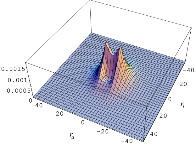
Figure 2: Conditional one-particle density function of the He₃ ground state, $r_{l}$ and $r_{a}$ are given in Å

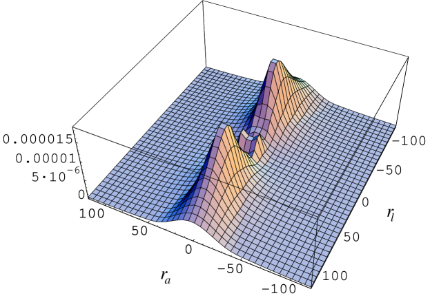
Figure 3: Conditional one-particle density function of the He₃ excited state, $r_{l}$ and $r_{a}$ are given in Å

is a projection to the orthogonal axis. Three-dimensional plots of the function $\rho((r_{l}^{2}+r_{a}^{2})^{1/2},\cos\arctan r_{l}/r_{a})$ corresponding to the ground and excited states of the trimer calculated with the LM2M2 potential are presented in Figs. 2 and 3 respectively. The conditional density function of the ground state decreases in all directions in a similar way. The density function of the excited state has two distinguishable maxima and exhibits the linear structure of the cluster. This structure has a simple physical explanation: The most probable positions of a particle in the excited state lie around the other two particles and when the latter particles are well separated the third one forms a dimer-like bound state with each of them. This interpretation agrees with the clusterisation coefficients presented in the Table 7. These coefficients are calculated as a norm of the function $f_{c}$ defined by

$$f_{c}(y)=\int\,{\rm d}x{\rm d}z\,\phi(x,y,z)\varphi_{2}(x)\,,$$ (22)

where $\varphi_{2}(x)$ is the dimer wave function. The values of $|f_{c}(y)|^{2}$, shown in the Table 7, demonstrate the dominating role of a two-body contribution to the trimer excited state whereas in the ground state this contribution is rather small. We could suppose that this dominating contribution of the cluster wave in the excited state ensured the fast convergence of the hyperspherical adiabatic expansion Fedorov to the correct value, but in order to get the same order of accuracy for the ground state, possibly more basic functions should be taken into account.

The advantage of using Faddeev equations over the Schrödinger one in bound-state calculations, is deduced from the results shown in Tables 8 and 9. In the latter table we present the contribution of different angular states to the Faddeev component and to the wave function calculated as

$$C_{n} = |f_{n}(x,y)|^{2}$$

$$f_{n}(x,y) = \int^{1}_{-1}{\rm d}z\,F(x,y,z)P_{n}(z)\,,$$ (23)

where $P_{n}(z)$, $n=0,2,4,\cdots$, are the Legendre polynomials and $F(x,y,z)$ is the Faddeev component or the wave function. The angular coefficients for the Faddeev component decrease much faster than the wave function coefficients. This could explain the difference between the estimations of the trimer mean square radius reported in Roudnev and the one presented here. In the previous paper the same angular basis for the Faddeev component and the wave function has been used. However, it turned out that the contribution of the higher partial waves to the wave function is not negligible. This leads, for instance, to the change of the mean square radius of the excited state for the LM2M2 potential from 60.85 Å to 59.3 Å. This observation agrees with the results of Nielsen et al. Fedorov , who reported the value 60.86 Å using essentially the same angular basis both for the wave function and for the Faddeev component. The Table 8 also demonstrates that more angular functions should be taken into account in the ground state calculations.

V Conclusions

We present a method which can be used to perform accurate three-body bound states calculations. It is specially suited for systems where the interparticle forces have a strong repulsive core. The method is based on Faddeev equations in the total angular momentum representation and without any further partial wave decomposition. The equations are expressed in terms of Cartesian coordinates which are best suited to describe the long-range behavior of weakly three-body bound states. Combined with the tensor-trick preconditioning for large linear systems and the Arnoldi’s algorithm for eigenanalysis it provided us accurate results for the the He₃ trimer bound and excited states.

Results obtained with the most recent realistic intermolecular forces (SAPT1, SAPT2, HFD-B3-FC11), as well as with earlier forces (LM2M2, TTYPT) indicate that only two bound states exist. The properties of these states are very different with the ground state being strongly bound while the binding energy for the excited state is comparable to that of the dimer. The latter implies that a dimmer cluster within the molecule is well formed.

The sizes of these two states also differs much. The characteristic size of the ground state either estimated by $\langle r\rangle$ or $\langle r^{2}\rangle^{1/2}$ is $\sim 10$ times less than the size of dimer molecule, but the size of the excited state has the same order of magnitude with that of the dimer. This estimation make it necessary to check for the absence of trimers in the experimental media during the measurement of dimer properties and vice versa.

Appendix A Reduction to a Linear System

Suppose $\tau_{t}=\{t_{0},t_{1},\ldots,t_{N_{t}}\}$ is a partition in the range $[t_{0},t_{N_{t}}]$ in coordinate $t$ and let $S_{5,2}(\tau_{t})$ be the space of quintique Hermite splines associated with this partition i.e. piecewise fifth order polynomial functions having two continuous derivatives in this range. The partition $\tau_{t}$ will be refereed to as the base grid. The set of basic functions in the space $S_{5,2}(\tau_{t})$ can be defined by the following conditions

$$S_{i}^{1}(t_{i})=1\,,\qquad\partial_{t}S_{i}^{1}(t_{i})=0\,,\qquad\partial^{2}_{t}S_{i}^{1}(t_{i})=0$$

$$S_{i}^{2}(t_{i})=0\,,\qquad\partial_{t}S_{i}^{2}(t_{i})=1\,,\qquad\partial^{2}_{t}S_{i}^{2}(t_{i})=0$$ (24)

$$S_{i}^{3}(t_{i})=0\,,\qquad\partial_{t}S_{i}^{3}(t_{i})=0\,,\qquad\partial^{2}_{t}S_{i}^{3}(t_{i})=1$$

$\forall t\notin[t_{\max(0,i-1),},t_{\min(i+1,N_{t})}]\>\Rightarrow\>S^{j}_{i}(t)=0$.

For simplicity we omit the subscript $\tau_{N_{t}}$ corresponding to any particular choice of a grid in each coordinate. Let the basic functions be arranged as follows:

$$\widehat{B}_{i}(t)=S^{j}_{k}(t)\,,\quad k=0\ldots N_{t}\,,\ \ j=1\ldots 3\,,\ \ i=3k+j-1$$ (25)

The solution of the Eq. (11) must satisfy Eq. (14) and vanish on the planes $x=0$ and $y=0$. To achieve this we modify the set of basic functions (24) by constructing linear combinations $B_{i}(t)$ which for $t=x,y$ read

$$B_{i}(t)\equiv\widehat{B}_{i}(t)\,,\qquad i=1\ldots 3N_{t}-1$$

(26)

$$B_{3N_{t}}(t)\equiv\widehat{B}_{3N_{t}}(t)-k_{t}\widehat{B}_{3N_{t}+1}(t)+k^{2}_{t}\widehat{B}_{3N_{t}+2}(t)$$

and for the coordinate $z$ they coincide with the initial basic functions (25) $B_{i}(z)=\widehat{B}_{i}(z)$. We look for an approximate solution of Eq. (11) in the form of expansion in terms of the basic functions (26)

$$\phi^{0}(x,y,z)=\sum_{i}f_{i}B_{i}(x,y,z)$$ (27)

where $i$ stands for the multi–index $\{i_{x},i_{y},i_{z}\}$ and $B_{i}(x,y,z)=B_{i_{x}}(x)B_{i_{y}}(y)B_{i_{z}}(z)$. Since the basic functions (26) fulfill the boundary conditions (14) these conditions are also satisfied by the approximate component $\phi^{0}$.

To obtain a system of equations for the coefficients $f_{i}$ the expansion (27) should be substituted into Eq. (11) with some subsequent projection procedure. A reasonable choice of such a procedure is the method of orthogonal collocations which do not require any integration. The highest order of approximation is achieved by a careful choice of collocation points for a given basic grid $\tau$ deBoorSwartz . For the grids $\tau_{N_{x}}$, $\tau_{N_{y}}$ and $\tau_{N_{z}}$ one should construct the grids of collocation points $\tau_{N^{c}_{x}}=\{x^{c}_{1},x^{c}_{2},\ldots,x^{c}_{N^{c}_{x}}\}$, $\tau_{N^{c}_{y}}=\{y^{c}_{1},y^{c}_{2},\ldots,y^{c}_{N^{c}_{x}}\}$, and $\tau_{N^{c}_{z}}=\{z^{c}_{1},z^{c}_{2},\ldots,z^{c}_{N^{c}_{x}}\}$ containing $N^{c}_{x}=3N_{x}$, $N^{c}_{y}=3N^{c}_{y}$, and $N^{c}_{z}=3(N_{z}+1)$ points respectively. Given these collocation grids the matrix elements of the operators involved in Eq. (11) can be easily constructed. For example, the matrix elements of the identity operator are $[I]_{ij}=B_{i}(x^{c}_{j_{x}},y^{c}_{j_{y}},z^{c}_{j_{z}})$ with $i=\{i_{x},i_{y},i_{z}\}$ and $j=\{j_{x},j_{y},j_{z}\}$.

Substituting the expansion (27) into Eq. (11) followed by the orthogonal collocation procedure one gets a system of linear algebraic equations

$$(\hat{H}^{0}_{0}+\hat{V}(\hat{I}+\hat{P})-E\hat{I}){\bf f}=0\>.$$ (28)

where $\hat{H}^{0}_{0}$, $\hat{V}$, $\hat{I}$, and $\hat{P}$ are the matrices corresponding to the operators of Eq. (11) while $\bf f$ is the coefficient vector of the expansion (27).

The dimension of this system is rather large and equals $N=N^{c}_{x}N^{c}_{y}N^{c}_{z}$. Therefore, we use this system of equations to find only its lowest generalized eigenvalues and eigenvectors.

Appendix B The Tensor-trick for Cartesian Coordinates

The inversion procedure of the operator $(\hat{H}_{1}-E\hat{I})$ is crucial for the performance of the algorithm and therefore a brief description of a tensor-trick algorithm for the DFE in Cartesian coordinates will be given. Furthermore, as the matrices involved are large, certain comments will be passed concerning the efficiency in computation.

Consider the Hamiltonian $\hat{H}_{1}=\hat{H}^{0}_{0}+\hat{V}\hat{I}$. The structure of this operator is

$$\widehat{I} = \widehat{I}_{x}\otimes\widehat{I}_{y}\otimes\widehat{I}_{z}$$

$$\widehat{H}_{1} = \widehat{D}_{x}\otimes\widehat{I}_{y}\otimes\widehat{I}_{z}+\widehat{I}_{x}\otimes\widehat{D}_{y}\otimes\widehat{I}_{z}$$

$$+ \widehat{I}_{x}\otimes\widehat{I}_{y}\otimes\widehat{1}_{z}\,(\widehat{L}_{x}\otimes\widehat{1}_{y}+\widehat{1}_{x}\otimes\widehat{L}_{y})\otimes\widehat{D}_{z}+\widehat{V}\widehat{I}_{x}\otimes\widehat{I}_{y}\otimes\widehat{I}_{z}\,.$$

The $\hat{I}_{t}$ are the matrices corresponding to the identity operators acting in coordinate $t$, $\hat{1}_{t}$ is the unit matrix, and $\hat{D}_{t}$ contains the elements of the corresponding differential operators. The tensor structure of the operator $\hat{H}$ allows a diagonalisation of it without solving the spectral problem in the $N$–dimensional space. To perform this diagonalisation one introduces the following matrices $\widehat{B}_{z}$, $\widehat{B}_{x}^{i}$, $\widehat{B}^{i}_{y}$ constructed from the generalized eigenvectors of the operators acting in different coordinates,

$$\widehat{B}_{z}\ : \ \widehat{D}_{z}\widehat{B}_{z}\,=\,\widehat{L}_{z}\widehat{I}_{z}\widehat{B}_{z}$$

$$\widehat{B}^{i}_{x}\ : \ (\widehat{D}_{x}+\widehat{V}\widehat{I}_{x}+l_{i}\widehat{L}_{x}\widehat{I}_{x})\widehat{B}^{i}_{x}\,=\,\widehat{X}^{i}\widehat{I}_{x}\widehat{B}^{i}_{x}$$

$$\widehat{B}^{i}_{y}\ : \ (\widehat{D}_{y}+l_{i}\widehat{L}_{y}\widehat{I}_{y})\widehat{B}^{i}_{y}\,=\,\widehat{Y}^{i}\widehat{I}_{y}\widehat{B}^{i}_{y}$$

where $\hat{L}_{z}={\rm diag}\{l_{1},l_{2},\ldots,l_{Nz}\}$, $\widehat{X}^{i}={\rm diag}\{E^{i}_{x1},E^{i}_{x2},\ldots,E^{i}_{xN_{x}}\}$, and $\widehat{Y}^{i}\,=\,{\rm diag}\{E^{i}_{y1},E^{i}_{y2},\ldots,E^{i}_{yN_{y}}\}$, and $E^{i}_{tN_{t}}$ are the eigenvalues of the corresponding operators. One also defines the matrices $\widehat{B}_{z}^{*}$, $\widehat{B}_{x^{i}}^{*}$, $\widehat{B}_{i_{y}}^{*}$ constructed of the eigenvectors of the adjoined equations. Expanding the expression $\hat{B}^{*}(\hat{H}_{1}-E\hat{I})\hat{B}$, with $\hat{B}$ and $\hat{B}^{*}$ being given by

$$\widehat{B} \equiv \prod^{N_{z}}_{i=1}\oplus(\widehat{B}^{i}_{x}\otimes\widehat{B}^{i}_{y})\otimes\widehat{[B}_{z}]_{i}$$

$$\widehat{B}^{*} \equiv \prod^{N_{z}}_{i=1}\oplus(\widehat{B^{i}}^{*}_{x}\otimes\widehat{B^{i}}^{*}_{y})\otimes\widehat{[B}^{*}_{z}]_{i}\,,$$

and taking into account the relation $\hat{B}^{*}\hat{B}=\hat{1}_{x}\otimes\hat{1}_{y}\otimes\hat{1}_{z}$, one can prove that the matrices $\hat{B}$ and $\hat{B}^{*}$ are the desired matrices diagonalising the operator $(\hat{H}_{1}-E\hat{I})$. Once this operator is diagonalised it can then be easily inverted

$$\widehat{B}^{*}(\hat{H}_{1}-E\hat{I})\widehat{B}=\widehat{G}\,,$$

$$(\hat{H}_{1}-E\hat{I})^{-1}=\widehat{B}\widehat{G}^{-1}\widehat{B}^{*}\,$$

$$\widehat{G}={\rm diag}\{g_{111},g_{112},\ldots,g_{i_{x}i_{y}i_{z}},\ldots,g_{N_{x}N_{y}N_{z}}\}$$

$$g_{i_{x}i_{y}i_{z}}=E^{i_{z}}_{xi_{x}}+E^{i_{z}}_{xi_{y}}-E$$

Thus, in principle, the task of construction of the operator $(\hat{H}_{1}-E\hat{I})^{-1}$ is over. However, to use computer power effectively one must care about optimal implementation of all the operations involved in the computation of the product of the operator $\hat{h}^{-1}(E)\equiv(\hat{H}_{1}-E\hat{I})^{-1}$ and a vector ${\bf u}$, the number of arithmetic operations should be minimized. To implement the operation effectively the structure of the operator $\hat{h}^{-1}(E)$ can be used

$$\hat{h}^{-1}(E)\equiv\widehat{B}\widehat{G}^{-1}(E)\widehat{B}^{*}\,.$$

The matrix $\widehat{G}^{-1}(E)$ has explicit diagonal structure, and the calculation of the product $\widehat{G}^{-1}{\bf u}$ requires only $O(N_{x}N_{y}N_{z})$ operations. Since however, the matrices $\widehat{B}$ and $\widehat{B}^{*}$ are dense, and in principle the calculation of the products $\widehat{B}^{(*)}{\bf u}$ requires $O((N_{x}N_{y}N_{z})^{2})$ arithmetic operations, that could essentially decrease the effectiveness of the method. However, taking into account the structure of the matrices $\widehat{B}$ and $\widehat{B}^{*}$ one can improve the performance. Consider the procedure of tensor multiplication of two matrices by a vector ${\bf u}$:

$${\bf v}=\widehat{B_{x}}\otimes\widehat{B_{y}}{\bf u}\,,$$

and use the identity

$$\widehat{B_{x}}\otimes\widehat{B_{y}}=\widehat{I}\otimes\widehat{B_{y}}\widehat{B_{x}}\otimes\widehat{I}\,.$$

Obviously, even the calculation of the product $\widehat{B_{x}}\otimes\widehat{B_{y}}{\bf u}$ requires $N^{2}_{x}N^{2}_{y}$ operations, the calculation of the products $\widehat{I}\otimes\widehat{B_{y}}{\bf u}$ and $\widehat{B_{x}}\otimes\widehat{I}{\bf u}$ require correspondingly only $N^{2}_{x}N_{y}$ and $N_{x}N^{2}_{y}$ operations. Therefore a multiplication of a tensor product by a vector would cost $N_{x}N_{y}(N_{x}+N_{y})$ operations. Similar relations can be written for a direct sum. Thus the correct implementation of a direct sum multiplication by a vector can reduce the computation costs $N_{x}N_{y}N_{z}/(N_{x}+N_{y}+N_{z})$ times.

The computation costs can be reduced even further. One of the possibilities is to abandon full diagonalisation of the operator $\widehat{h}(z)$ and to modify the computation scheme. For this, let us construct the matrices diagonalising only the terms corresponding to the coordinates $y$ and $z$

$$\tilde{B}\equiv\prod^{N_{z}}_{i=1}\oplus(\widehat{I}\otimes\widehat{B^{i}}_{y})\otimes\widehat{[B_{z}]}_{i}\,,$$

$$\tilde{B}^{*}\equiv\prod^{N_{z}}_{i=1}\oplus(\widehat{I}\otimes\widehat{B^{i}}^{*}_{y})\otimes\widehat{[B^{*}_{z}]}_{i}\,.$$

In this case the matrix $\tilde{G}(z)\equiv\tilde{B}^{*}\widehat{h}(z)\tilde{B}$ is band because of the fact that the operator is local and the basic functions have well localized support (26). The multiplication $\widehat{L}(z){\bf u}$ can be performed in two stages:

• Solve a system of equations with a band matrix $\tilde{G}(E)$

  $$\tilde{G}(z)\tilde{{\bf u}}=\tilde{B}^{*}(\widehat{V}\widehat{P}+\widehat{V}_{c}\widehat{S}){\bf u}\,;$$

• calculate ${\bf v}\equiv\widehat{L}(z){\bf u}$ as

  $${\bf v}=\tilde{B}\tilde{{\bf u}}\,.$$

Taking into account the tensor structure of the matrices $\tilde{B}^{*}$ and $\tilde{B}$ this computation scheme requires only $O(N_{x}\,N_{y}\,N_{z}\,(N_{y}+N_{z}))$ operations.

Appendix C Convergence rates for the Arnoldi algorithm

The key point of this algorithm is the repeated action of the operator under consideration on a sequence of vectors generating a Krylov subspace where the desired eigenvector lies. To use this algorithm to solve the eigenvalue problem (18) one must be able to calculate the action of the operators $(\hat{H}_{1}-E\hat{I})^{-1}$ and $\hat{H}_{2}$ on an arbitrary vector ${\bf u}$. Thus the problems of inversion of the operator $(\hat{H}_{1}-E\hat{I})$ and storage of the matrix $\hat{H}_{2}$ should be solved first. In Ref. Groning hyperspherical coordinates were used which lead to an effective storage scheme for the matrices $\hat{H}_{2}=\hat{V}(\hat{I}+\hat{P})$. However, one can not include pair interaction into the invertible part $(\hat{H}_{1}-E\hat{I})$ using hyperspherical coordinates. On the other hand, if Cartesian coordinates are used then one has difficulties with the storage of the matrix $\hat{P}$ since these coordinates do not have the same symmetry properties as the operator $P$ and this results to an irregular structure of $\hat{P}$. In our case the situation is saved by the total angular momentum representation. In contrast to bispherical expansion used in Groning , the operator $P$ is local and does not contain any terms requiring integration. As a result the matrix $\hat{P}$ is sparse and can be either effectively stored using any standard storage scheme for sparse matrices sparce or not stored at all. In the last case the matrix elements are calculated “on fly” when required.

The estimations of the convergence rate of the Arnoldi algorithm Saad are essential in understanding the problems that arise when the tensor-trick algorithm is applied. Suppose $\hat{L}$ is a linear operator in a finite-dimensional space with

$$\hat{L}{\bf u}_{i}=\lambda_{i}{\bf u}_{i}\,.$$

Let ${\cal K}_{m}(\bf v)$ be a Krylov subspace of dimension $m$ constructed from a starting vector $\bf v$ of the operator $\hat{L}$ and ${\cal P}_{m}$ be an orthogonal projector to ${\cal K}_{m}$ space. The convergence rate of the algorithm can be expressed in terms of the norm

$$\varepsilon_{i}^{(m)}\equiv||(1-{\cal P}_{m}){\bf u}_{i}||$$

of the eigenvector $u_{i}$ projection onto the orthogonal completion to ${\cal K}_{m}$. Suppose $\alpha_{k}$ are the expansion coefficients of the starting vector ${\bf v}$ in terms of the eigenvectors ${\bf u}_{i}$,

$${\bf v}=\sum_{i=1}^{n}\alpha_{i}{\bf u}_{i}\,.$$

Then the following relation is fulfilled

$$\varepsilon_{i}^{(m)}\leq\xi_{i}\epsilon_{i}^{(m)}\,,$$

where $\xi_{i}=-1+\sum_{k=1}^{n}|\alpha_{k}|/|\alpha_{i}|$ and $\epsilon_{i}^{(m)}$ depends on the spectral properties of the operator $\hat{L}$. For the eigenvalues lying in the external part of the spectrum some practically important estimations are known. Suppose that all the eigenvalues of $\hat{L}$ but $\lambda_{1}$ lye inside of an ellipse with the center $c$, largest semi-axis $a$, and focuses $c\pm e$. It can then be shown that $\epsilon_{1}^{(m)}$ satisfy the following estimation Saad

$$|\epsilon_{1}^{(m)}|\leq\frac{C_{m-1}(\displaystyle\frac{a}{e})}{C_{m-1}(\displaystyle\frac{\lambda_{1}-c}{e})}\ ,$$

where $C_{m}(t)$ are Chebyshev polynomials of the first kind.

Consider now the convergence rate of Arnoldi algorithm for the operator $\hat{L}(z)$ (19) for the value of z corresponding to the ground state of a three-body system. In this case the maximal eigenvalue $\lambda_{1}=1$. Having defined the separation distance between the largest eigenvalue and the rest part of the spectrum $s\equiv|1-\lambda_{2}|$, the distance between the maximal eigenvalues in the rest part $d\equiv|\lambda_{2}-\lambda_{n}|$ and neglecting the imaginary part of the spectrum, we obtain the estimation

$$|\epsilon_{1}^{(m)}|\leq|C_{m-1}(1+\frac{2s}{d})|^{-1}\ .$$

Therefore the parameter managing the convergence rate is the ratio $s/d$ of the separation to the size of the rest part of the spectrum. The convergence rate could be improved by enlarging the separation and by enhancing the remainder part of the spectrum localization.

Table 1: Bound state energies for the helium dimer He₂ and trimer He₃: $E_{2}^{\rm ex}$ and $E_{2}$ are the exact and calculated (using the same grid employed in three-body calculations) two-body bound states while $E_{3}$ and $E_{3}^{*}$ are the ground and excited states for the trimer.

Potential	$E_{2}^{\rm ex}$ (mK)	$E_{2}$ (mK)	$E_{3}$ (K)	$E^{*}_{3}$ (mK)
SAPT1Az97	-1.732405	-1.7322	-0.13382	-2.790
SAPT2Az97	-1.815003	-1.8146	-0.13516	-2.888
SAPT Az97	-1.898390	-1.8979	-0.13637	-2.986
LM2M2Az91	-1.303482	-1.304	-0.12641	-2.271
TTYPTTTY	-1.312262	-1.3121	-0.12640	-2.280
HFD-B3-FC11Az97	-1.587301	-1.5873	-0.13126	-2.617

Table 2: Convergence for the He₃ ground state energy with respect to the number of grid points for the LM2M2 potential.

Grid	$E_{3}$ (K)	$E_{2}$ (mK)
45$\times$45$\times$6	-0.12570	-1.3002
60$\times$60$\times$6	-0.12583	-1.3032
75$\times$75$\times$6	-0.12582	-1.3034
90$\times$90$\times$6	-0.12582	-1.3035
105$\times$105$\times$6	-0.12581	-1.3034
105$\times$105$\times$9	-0.12636	-1.3034
105$\times$105$\times$12	-0.12636	-1.3034
105$\times$105$\times$15	-0.12640	-1.3034
105$\times$105$\times$18	-0.12640	-1.3034

Table 3: Same as in Table 2 but for the excited state.

Grid	$E^{*}_{3}$ (mK)	$E_{2}$ (mK)
45$\times$45$\times$6	-2.2658	-1.3011
60$\times$60$\times$6	-2.2649	-1.3018
75$\times$75$\times$6	-2.2668	-1.3031
90$\times$90$\times$6	-2.2670	-1.3031
105$\times$105$\times$6	-2.2677	-1.3037
105$\times$105$\times$9	-2.2712	-1.3037
105$\times$105$\times$12	-2.2707	-1.3037
105$\times$105$\times$15	-2.2707	-1.3037

Table 4: Comparison of the results obtained with the LM2M2 potential with other results in the field.

Observable	This work	Fedorov	Moto2
$E_{3}$, K	-0.1264	-0.1252	-0.1259
$E^{*}_{3}$, mK	-2.271	-2.269	-2.28
$<r^{2}>^{1/2}$, Å	6.32	6.24
$<r^{2}_{*}>^{1/2}$, Å	59.3	60.86

Table 5: The mean radius of He₃ in Å

Potential	Ground state of He3	Excited state of He3	He2
SAPT1	5.47	47.5	45.60
SAPT2	5.45	47.1	44.63
SAPT	5.44	47.1	43.73
HFD-B3-FC11	5.49	48.3	47.47
LM2M2	5.55	49.9	52.00
TTYPT	5.55	50.1	51.84

Table 6: The mean square radius of He₃ in Å

Potential	Ground state	Excited state	He2
SAPT1	6.22	56.4	61.89
SAPT2	6.21	55.9	60.52
SAPT	6.19	55.9	59.24
HFD-B3-FC11	6.26	57.4	64.53
LM2M2	6.32	59.3	70.93
TTYPT	6.33	59.6	70.70

Table 7: Contribution of cluster wave to the Faddeev component

Potential	$\|f_{c}\|^{2}$	$\|f_{c}^{*}\|^{2}$
SAPT1	0.2743	0.9442
SAPT2	0.2787	0.9461
SAPT	0.2832	0.9478
HFD-B3-FC11	0.2661	0.9407
LM2M2	0.2479	0.9319
TTYPT	0.2487	0.9323

Table 8: Contribution of different two-body angular states to the Faddeev component

	Ground state			Excited state
Potential	S	D	G	S	D	G
SAPT1	0.9989914	0.0009974	0.0000108	0.9999951	0.0000049	0.0000001
SAPT2	0.9989822	0.0010065	0.0000109	0.9999950	0.0000050	0.0000001
SAPT	0.9989754	0.0010131	0.0000111	0.9999949	0.0000050	0.0000001
HFD-B3-FC11	0.9990060	0.0009830	0.0000106	0.9999953	0.0000047	0.0000000
LM2M2	0.9990393	0.0009500	0.0000103	0.9999956	0.0000043	0.0000000
TTYPT	0.9990332	0.0009561	0.0000104	0.9999956	0.0000043	0.0000000

Table 9: Contribution of different two-body angular states to the wave function

	Ground state			Excited state
Potential	S	D	G	S	D	G
SAPT1	0.9521	0.0336	0.0089	0.855	0.099	0.031
SAPT2	0.9520	0.0338	0.0090	0.854	0.100	0.031
SAPT	0.9519	0.0339	0.0090	0.826	0.102	0.034
HFD-B3-FC11	0.9525	0.0335	0.0089	0.837	0.100	0.033
LM2M2	0.9530	0.0329	0.0089	0.873	0.093	0.025
TTYPT	0.9527	0.0332	0.0094	0.862	0.094	0.029

(a) TTYPT potential

(b) MT-V potential

Figure 1: Spectra of operators $\hat{L}(E)$ for potentials with (a) and without (b) a strong repulsive core

References

- (1) E. Nielsen, D. V. Fedorov, and A. S. Jensen, J. Phys. B, 31, 4085 (1998).
- (2) V. Roudnev and S. L. Yakovlev, Chem. Phys. Lett. 328, 97 (2000).
- (3) E. A. Kolganova, A. K. Motovilov, S. A. Sofianos, J. Phys. B, 31, 1279 (1998).
- (4) H. P. Noyes and H. Fiedelday Calculations of three-nucleon low-energy parameters, in Three-particle scattering in Quantum Mechanics, 195 (1968).
- (5) A. Laverne and C. Gignoux, Nucl. Phys. A203, 597 (1973).
- (6) S. P. Merkuriev, C. Gignoux, and A. Laverne, Ann. Phys. 99, 30 (1976).
- (7) G. L. Payne, J. L. Friar, B. F. Gibson, and I. R. Afnan, Phys. Rev. C 22, 823 (1980).
- (8) A. Kvitsynsky and C. Y. Hu, Few-Body Systems 12, 7 (1992).
- (9) S. L. Yakovlev and I. N. Filikhin, Sov. J. Nucl. Phys. 56/12, 98 (1993).
- (10) S. P. Merkuriev, Theor. Math. Phys. 8, 235 (1971); 32, 187 (1977) (in Russian).
- (11) N. W. Schellingerhout, L. P. Kok, and G. D. Bosveld Phys. Rev. A 40, 5568 (1989).
- (12) L. P. Kok, N. W. Schellingerhout Few-Body Systems 11, 99 (1991).
- (13) J. Carbonell, C. Gignoux, and S. P. Merkuriev, Few–Body Systems 15, 15 (1993).
- (14) V. V. Kostrykin, A. A. Kvitsinsky, and S. P. Merkuriev, Few-Body Systems 6, 97 (1989).
- (15) L. D. Faddeev and S. P. Merkuriev, Quantum scattering theory for several particle systems (Doderecht: Kluwer Academic Publishers, (1993)).
- (16) C. de Boor and B. Swartz, SIAM J. Numer. Anal. 10, 582 (1973).
- (17) Y. Saad, Numerical methods for large eigenvalue problems, Manchester University Press in Algorithms and architectures for Advanced Scientific Computing, NY (1992).
- (18) R. A. Malfliet and J. A. Tjon, Nucl. Phys. A127, 161 (1969).
- (19) K. T. Tang, J. P. Toennis, and C. L. Yiu, Phys. Rev. Lett. 74, 1546, (1995).
- (20) A. R. Janzen and R. A. Aziz, J. Chem. Phys. 107, 914 (1997).
- (21) R. A. Aziz and M. J. Slaman, J. Chem. Phys. 94, 8047 (1991).
- (22) A. K. Motovilov, W. Sandhas, S. A. Sofianos, and E. A. Kolganova, Eur. Phys. J D, 13, 33 (2001).
- (23) A. K. Motovilov, W. Sandhas, S. A. Sofianos, and E. A. Kolganova, Nucl Phys. A684, 646c (2001).
- (24) Y. Saad, SPARSKIT: A basic tool kit for sparse matrix computations. Technical report, Computer Science Department, University of Minnesota, Minneapolis, MN 55455, June 1994.