Stochastic Transition between Turbulent Branch and
Thermodynamic Branch of an Inhomogeneous Plasma

Abstract

Transition phenomena between thermodynamic branch and turbulent branch in submarginal turbulent plasma are analyzed with statistical theory. Time-development of turbulent fluctuation is obtained by numerical simulations of Langevin equation which contains submarginal characteristics. Probability density functions and transition rates between two states are analyzed. Transition from turbulent branch to thermodynamic branch occurs in almost entire region between subcritical bifurcation point and linear stability boundary.

1 Introduction

There have been observed various kinds of formations and destructions of transport barriers. Both in edge and internal regions of high temperature plasmas, the dynamical change often occurs on the short time scale, sometimes triggered by subcritical bifurcation. These features naturally lead to the concept of transition [1].

The transition takes place as a statistical process in the presence of statistical noise source which is induced by strong turbulence fluctuation. As a generic feature, the transition occurs with a finite probability when a controlling parameter approaches the critical value.

The nonequilibrium statistical mechanics, which deals with dynamical phase transitions and critical phenomena, should be extended for inhomogeneous plasma turbulence [2]. To this end, statistical theory for plasma turbulence has been developed and stochastic equations of motion (the Langevin equations) of turbulent plasma were derived [3]. The framework to calculate the probability density function (PDF), the transition rates etc. have also been made.

In this paper, we apply the theoretical algorithm to an inhomogeneous plasma with the pressure gradient and the shear of the magnetic field. Microturbulence in the system is known to be subcritically excited from the thermodynamic branch [4]. The transition between the thermodynamic branch and the turbulent branch is studied. We show that the transition occurs stochastically by numerically solving the Langevin equation of the turbulent plasmas. In order to characterize the stochastic nature of the transition, the frequency of occurrence of a transition per unit time (the transition rate) is calculated as a function of the pressure-gradient and the plasma temperature. The results show that the transition from the turbulent branch to the thermodynamic branch occurs in a wide region instead of at a transition point.

2 Theoretical Framework

In this section, we briefly review the theoretical framework [3] used in our analysis of turbulent plasmas.

The theory is based on the Langevin equation, eq. (1), derived by renormalizing with the direct-interaction approximation the reduced MHD for the three fields: the electro-static potential, the current and the pressure. The Langevin equation gives the time-development of the fluctuating parts of the three fields as

$$\frac{\partial\mathbf{f}}{\partial t}+\hat{\cal L}\mathbf{f}=\mathbf{\cal N}(t),\ \mbox{where}\ \mathbf{f}(t)\equiv\left(\begin{array}[]{c}\phi(t)\\ J(t)\\ p(t)\end{array}\right).$$ (1)

In this equation, the nonlinear terms are divided into two parts: One part is coherent with the test field $\mathbf{f}(t)$ and is included into the renormalized operator $\hat{\cal L}$. The other is incoherent and is modeled by a random noise $\mathbf{\cal N}(t)$. Since $\mathbf{\cal N}(t)$ is a force which fluctuates randomly in time, the Langevin equation describes the stochastic time-development of the fluctuation of the three fields.

By analyzing the Langevin equation eq. (1), a number of statistical properties of turbulent plasmas can be derived. For example, the analytical formulae for the change rate of plasma states, the transition rates, were derived. Furthermore, since the renormalized transport coefficients come from the term of the random force $\mathbf{\cal N}(t)$, relations between the fluctuation levels of turbulence and the transport coefficients like the viscosity and the thermal diffusivity were derived.

3 A Model

With the theoretical framework briefly described in the previous section, we analyze a model of inhomogeneous plasmas with the pressure-gradient and the shear of the magnetic field [3]. The model is formulated with the reduced MHD for the three fields of the electro-static potential, the current and the pressure. The shear of the magnetic field is given as $\mathbf{B}=(0,B_{0}sx,B_{0})$ where $B_{0}(x)=\mbox{const}\times(1+\Omega^{\prime}x+\cdots)$. The pressure is assumed to change in $x-$direction.

It has been known that in this system bifurcation due to the subcritical excitation of the current diffusive interchange mode (CDIM) occurs [4] as shown in Fig. 1.

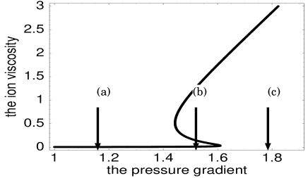
Figure 1: The dependence of the renormalized ion-viscosity on the pressure-gradient. It is clearly seen that the bifurcation between a low viscosity state (the thermodynamic branch) and a high viscosity state (the turbulent branch) occurs. The arrows indicate the typical values of the pressure-gradient where some physical quantities are evaluated in the rest of this paper.

Figure 1 shows the dependence of the turbulent ion-viscosity on the pressure-gradient. The turbulent ion-viscosity is proportional to the fluctuation level. Both the pressure-gradient and the turbulent viscosity are normalized. It is clearly seen that the bifurcation between a low viscosity state and a high viscosity state occurs. Due to the bifurcation, transition between the two states and hysteresis are expected to be observed. The low viscosity state is called “the thermodynamic branch”, since this state is continually linked to thermal equilibrium. We call the high viscosity state “the turbulent branch”, since the fluctuation level is also large in a strong turbulent limit [3]. The ridge point where the turbulent branch ends is denoted “the subcritical bifurcation point”. The region between the subcritical bifurcation point and the ridge near the linear stability boundary is called “the bi-stable regime”.

From the deterministic point of view, the transition from the thermodynamic branch to the turbulent branch is expected to occur only at the ridge point near the linear stability boundary and the transition in the opposite direction is expected to occur only at the subcritical bifurcation point.

4 Stochastic Occurrence of the Transition

Figure 2: (a) The coefficients $\lambda(\varepsilon)$ and $\eta(\varepsilon)$ in eq. (2) at (a) in Fig. 1. (b) $\lambda(\varepsilon)$ and $\eta(\varepsilon)$ at (b) in Fig. 1. (c) $\lambda(\varepsilon)$ and $\eta(\varepsilon)$ at (c) in Fig. 1.

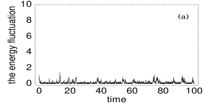
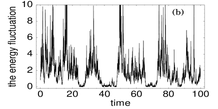
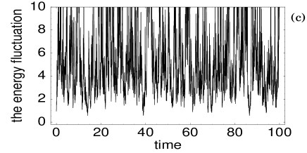
Figure 3: (a) A sample of a time-series of $\varepsilon(t)$ for the point (a) in Fig. 1. There is only small fluctuation since the system is always in the thermodynamic branch. (b) $\varepsilon(t)$ for the point (b) in Fig. 1. Bursts are observed intermittently. It means that the transition between the thermodynamic branch and the turbulent branch occurs stochastically. (c) $\varepsilon(t)$ for the point (c) in Fig. 1. Bursts occur simultaneously since the system in the turbulent branch.

In order to capture the characteristics of the two states, we concentrate on the time-development of the energy of fluctuation of the electric field, $\varepsilon(t)$. The quantity $\varepsilon(t)$ obeys the coarse-grained Langevin equation, eq. (2), which has been derived in ref. 3.

$$\frac{d}{dt}\varepsilon(t)=-2\lambda(\varepsilon)\varepsilon(t)+\eta(\varepsilon)R(t).$$ (2)

Here, $R(t)$ is assumed to be the Gaussian noise whose variance is unity. The coefficients $\lambda(\varepsilon)$ and $\eta(\varepsilon)$ depend on the pressure-gradient and the temperature and so the shapes of the functions for one regime of the pressure-gradient are completely different from that for the other regime. The shapes of $\lambda(\varepsilon)$ and $\eta(\varepsilon)$ for each of three regimes are shown in Fig. 2. For the detailed formulae of $\lambda(\varepsilon)$ and $\eta(\varepsilon)$, see ref. 5.

The essential point is that the function $\lambda(\varepsilon)$ takes both a positive and a negative value in the bi-stable regime (Fig. 2 (b)). So, the fluctuation of the electric field is suppressed when $\lambda(\varepsilon)$ is positive and it is excited when $\lambda(\varepsilon)$ is negative. Consequently, there are two metastable states in the bi-stable regime.

By solving numerically eq. (2), we obtain the following samples of a time-series for each of three values of the pressure-gradient (three points (a), (b) and (c) shown in Fig. 1). When the pressure-gradient is fixed at the value smaller than the subcritical bifurcation value ((a) in Fig. 1), there is only small fluctuation since the system is always in the thermodynamic branch as shown in Fig. 3 (a).

On the other hand, when the pressure-gradient takes a value in the bi-stable regime ((b) in Fig. 1), bursts are observed intermittently as shown in Fig. 3 (b). That is, transition between the thermodynamic branch and the turbulent branch occurs stochastically. The bursts correspond to the turbulent branch and the laminar corresponds to the thermodynamic branch. The fact that the residence times at the each states are random leads to the statistical description of the transition with the transition rates described in the rest of this paper.

When the value of the pressure-gradient is larger than that of the linear stability boundary ((c) in Fig. 1), bursts are always observed (see Fig. 3 (c)). It means that the system is always in the turbulent branch.

5 The Probability Density Functions

In order to characterize the random fluctuation shown in the last section, we introduce the probability density function (PDF) $P(\varepsilon)$ defined as the probability density that a random variable takes a certain value $\varepsilon$. PDFs often reveal the invisible structures hidden in randomly fluctuating data $\varepsilon(t)$.

By counting the frequency of realization of a certain value $\varepsilon$ from time-serieses of $\varepsilon(t)$ over sufficiently long time, the histogram is obtained. The PDF $P(\varepsilon)$ is the histogram normalized with the total frequency. So, in general, the PDF can be obtained from time-serieses observed in real experiments as a normalized histogram.

Figure 4 shows the PDFs for three regimes of the pressure-gradient obtained from the time-series shown in Fig. 3. Figure 3 (b) shows that transition frequently occurs between the turbulent branch and the thermodynamic branch. Dithering between these two states is observed also in the PDF as the two peaks in Fig. 4 (b).

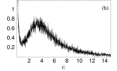
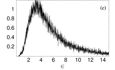
Figure 4: (a) The PDF when the value of the pressure-gradient is smaller than that of the subcritical bifurcation point ((a) in Fig. 1). The PDF takes a finite value only in the small $\varepsilon$ region. (b) The PDF when the value of the pressure-gradient is fixed in the bi-stable regime ((b) in Fig. 1). The two peaks are clearly seen, even though it is not clear from the time-series Fig. 3 (b) that there are two regions where the system is found frequently. (c) The PDF when the value of the pressure-gradient is larger than that of the linear stability boundary ((c) in Fig. 1). There is single peak corresponding to the turbulent branch.

Figure 5 (a) shows the tail of the PDF when the pressure-gradient is fixed at the value smaller than the subcritical bifurcation value. The PDF obeys the power-law for relatively large $\varepsilon$, even though the system is in the thermodynamic branch. The power-law tail when the value of the pressure-gradient is larger than that of the linear stability boundary is shown in Fig. 5 (b).

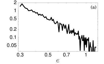
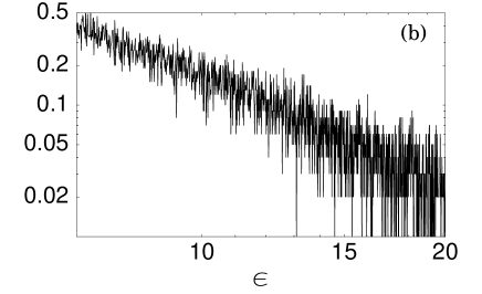
Figure 5: (a) The tail of the PDF when the pressure-gradient is fixed at the value smaller than the subcritical bifurcation value. The PDF obeys the power-law for relatively large $\varepsilon$, even though the system is in the thermodynamic branch. (b) The tail of the PDF when the value of the pressure-gradient is larger than that of the linear stability boundary. The PDF obeys the power-law when the system is in the turbulent branch.

It is important from the point of view of theoretical investigation to note that the PDFs are also obtained as solutions of the Fokker-Planck equation equivalent to the Langevin equation eq. (2).

6 The Transition Rates

In order to formulate the stochastic transition phenomena in the bi-stable regime, we introduce the transition rates. There are transitions in two opposite direction: the transition from the thermodynamic branch to the turbulent branch, which we call “the forward transition, and the transition in the opposite direction is called “the backward transition”. There are two transition rates. One is the forward transition rate $r_{f}$ which is the frequency of occurrence of the forward transition per unit time and the other is the backward transition rate $r_{b}$ defined similarly as the frequency of occurrence of the backward transition per unit time.

It is important to note that these quantities are observable quantities. It is easily shown that the forward transition rate is equal to the average of inverse of the residence time at the thermodynamic branch and the backward transition rate is equal to the average of inverse of the residence time at the turbulent branch. Therefore, these transition rates can be measured from the time-serieses of fluctuation.

We determine the value of the pressure-gradient with which the transition occurs frequently. The transition rates are calculated with the formulae derived in ref. 6. Figure 6 shows the dependence of the forward transition rate and the backward transition rate on the pressure gradient in the bi-stable regime, i.e., (b) in Fig. 1.

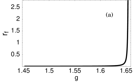
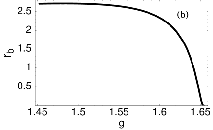
Figure 6: (a) The dependence of the forward transition rate per unit time on the normalized pressure-gradient, $g$, in the bi-stable regime. The left edge and the right edge of the horizontal axis corresponds to the subcritical bifurcation point and the linear stability boundary. It is seen that the forward transition occurs mainly in the vicinity of the linear stability boundary. (b) The dependence of the backward transition rate per unit time on the pressure gradient in the bi-stable regime. It is seen that the backward transition occurs in the almost entire bi-stable regime.

The forward transition triggered by the thermal noise occurs mainly in the vicinity of the linear stability boundary. In contrast, it is clearly seen that the backward transition occurs in the almost entire bi-stable regime in contrast to the expectation from the deterministic point of view of bifurcation phenomena. This behavior is due to strong turbulent fluctuation. It is noted that the backward transition, i.e. the transition in a turbulence, occurs in a “region” instead of a “point” of the parameter space.

7 Hysteresis Phenomena

Up to now, the value of the pressure-gradient is fixed. Next, in order to investigate hysteresis phenomena, we turn to the case when the pressure-gradient changes in time.

It is important to investigate this case, since the pressure-gradient can be a dynamical variable in realistic plasmas. Since the characteristic time-scale of the transition is given by the inverse of the transition rate, $1/r$, the effect of the change of the pressure-gradient is governed by the interrelation between the transition rate $r$ and the time-rate of the change of the pressure-gradient, $\dot{g}(t)$. When $|\dot{g}(t)/g(t)|\sim r$ or $|\dot{g}(t)/g(t)|>r$, the system cannot follow the change of the pressure-gradient $g(t)$. Then, the state of the system depends on the value of the pressure-gradient $g(t)$ in the past and hysteresis phenomena are expected to be observed.

On the other hand, when $|\dot{g}(t)/g(t)|\ll r$, the system can follow the change of the pressure-gradient $g(t)$. Since in this case the state of the system is the steady state for the value of the pressure-gradient at the moment, hysteresis phenomena cannot be observed.

The protocol to change the pressure-gradient is as follows (see Fig. 7.): At first the pressure-gradient is increased through the bi-stable regime and after that it is decreased to the original value. The time-rate of change of the pressure-gradient is assumed to be constant for simplicity. Furthermore, in order to observe hysteresis, the speed of change of the pressure-gradient is chosen so that it is of the same order of the transition rates or larger than that.

Figure 7: The protocol to change the pressure-gradient to analyze hysteresis phenomena. At first the pressure-gradient is increased through the bi-stable regime ($1.45<g<1.65$)and after that it is decreased to the original value ($g=1$). The time-rate of change of the pressure-gradient is assumed to be constant $|\dot{g}(t)|=0.1$ for simplicity.

Figure 8 (a) and (b) are the samples of hysteresis loops drawn by numerically solving the Langevin equation eq. (2). The dashed lines show $\varepsilon$ when the pressure-gradient is increased and the solid lines show $\varepsilon$ when the pressure-gradient is decreased. These figures, Fig. 8 (a) and (b), are obtained for the exactly same temperature and the time-rate of change of the pressure-gradient. The forward transition occurs around at $g=1.65$ in both cases shown in Fig. 8 (a) and (b). However, the backward transition point shown in Fig. 8 (a) around at $g=1.5$ is completely different from the transition point around $g=1.6$ shown in Fig. 8 (b). It is because the backward transition can occur in the almost entire bi-stable regime as shown in the analysis of the backward transition rate (see Fig. 6 (b)). Consequently, the backward transition point changes stochastically from case to case. Since the distribution of the transition point is due to strong turbulent fluctuation, it is expected in general that transition points between different turbulent branches are distributed stochastically. We expect that distribution of the L/H transition point observed in real experiments [7] is explained in this direction.

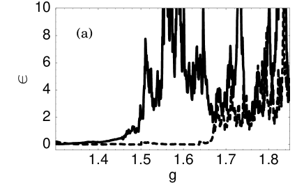
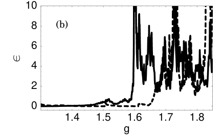
Figure 8: (a) A sample of the hysteresis loop drawn by numerically solving the Langevin equation eq. (2). The dashed line show $\varepsilon$ when the pressure-gradient is increased and the solid line show $\varepsilon$ when the pressure-gradient is decreased. (b) The other sample of the hysteresis loop obtained for the exactly same temperature and the time-rate of change of the pressure-gradient for Fig. 8 (a). Since the backward transition can occur in the almost entire bi-stable regime, the backward transition point is different from that of Fig. 8 (a).

8 Summary and Discussion

Summarizing our work, we applied the statistical theory of plasma turbulence to problems of the transition phenomena of submarginal turbulence. By numerically solving the Langevin equation, the typical time-development of fluctuation is obtained. It tells that the transition for the model of inhomogeneous plasma occurs stochastically and suggests how the transition phenomena due to subcritical bifurcation may look in time-serieses obtained in real experiments.

Furthermore, we obtained the PDFs of $\varepsilon(t)$ and the pressure-gradient dependence of the transition rates. It is shown that the backward transition occurs with almost equal frequency in the entire bi-stable regime, so the transition occurs in a “region”. The concept “transition region” is necessary in the analysis of data obtained by real experiments. It is confirmed that the backward transition does not occur only at the bifurcation point but occur also in the region of the pressure-gradient by observing the hysteresis loops obtained by numerically solving the Langevin equation.

It is important to discuss whether the transition phenomena considered in this paper can be observed in real experiments. Since the characteristic time-scale of the transition is given by the inverse of the transition rate, observability depends on the interrelation between the time resolution of observation $\triangle t$ and the transition rate $r$. When $\triangle t$ is much smaller than $1/r$, the transition phenomena as shown in Fig. 3 (a) are expected to be observed. On the other hand, when $\triangle t$ is of the same order of $1/r$ or larger than $1/r$, transition phenomena average out and only the average over $\triangle t$ is observed. This discussion is generic regardless of the type of transition, e.g. the transition between the thermodynamic branch and the turbulent branch, L/H transition etc.

References

- [1] For a review of theoretical modeling of transport barriers, see, e.g., S.-I. Itoh, K. Itoh and A. Fukuyama: J. Nucl. Mater. 222 (1995) 117; K. Itoh and S.-I. Itoh: Plasma Phys. Control. Fusion 38 (1996) 1; M. Wakatani: ibid. 40 (1998) 597; J. W. Connor and H. R. Wilson: ibid. 42 (2000) R1; P. W. Terry: Rev. Mod. Phys. 72 (2000) 109; A. Yoshizawa, S.-I. Itoh, K. Itoh and N. Yokoi: Plasma Phys. Contr. Fusion 43 (2001) R1.
- [2] See, e.g., R. Kubo, M. Toda and N. Hashitsume: Statistical Physics II (Springer, Berlin, 1985); R. Balescu, Equilibrium and Nonequilibrium Statistical Mechanics (Wiley, NY, 1975).
- [3] S.-I. Itoh and K. Itoh: J. Phys. Soc. Jpn. 68 (1999) 1891; ibid. 68 (1999) 2611; ibid. 69 (2000) 408; ibid. 69 (2000) 427; ibid. 69 (2000) 3253.
- [4] K. Itoh, S.-I. Itoh, M. Yagi and A. Fukuyama: Plasma Phys. Control. Fusion 38 (1996) 2079.
- [5] S.-I. Itoh and K. Itoh: J. Phys. Soc. Jpn. 68 (1999) 2611.
- [6] S.-I. Itoh and K. Itoh: J. Phys. Soc. Jpn. 69 (2000) 427.
- [7] ITER H-mode database working group: Nucl. Fusion 34 (1994) 131.