Numerical estimation of entropy loss on dimerization: improved prediction of the quaternary structure of the GCN4 leucine zipper

Abstract

A lattice based model of a protein is used to study the dimerization equilibrium of the GCN4 leucine zipper. Replica exchange Monte Carlo is used to determine the free energy of both the monomeric and dimeric forms as a function of temperature. The method of coincidences is then introduced to explicitly calculate the entropy loss associated with dimerization, and from it the free energy difference between monomer and dimer, as well as the corresponding equilibrium reaction constant. We find that the entropy loss of dimerization is a strong function of energy (or temperature), and that it is much larger than previously estimated, especially for high energy states. The results confirm that it is possible to study the dimerization equilibrium of GCN4 at physiological concentrations within the reduced representation of the protein employed.

I Introduction

Reduced models of a protein have been shown to provide a possible route for the estimation of the free energy of dimerization of relatively short coiled-coils [1, 2, 3]. A key step in the calculation of the free energy of dimerization concerns the entropy loss upon bringing two monomer chains together to form the dimer. A practical method for the numerical estimation of this entropy loss by Monte Carlo simulation is discussed in this paper.

The focus of our work is on the calculation of free energies of dimerization, and in particular a re-analysis (using a subsequently improved model) of prior research about the folding thermodynamics of the GCN4 leucine zipper [2, 3]. Leucine zippers belong to the class of structural motifs that are known as coiled coils. Generically, they comprise right handed $\alpha$ helices wrapped around each other with a small left-handed super-helical twist [4]. While leucine zippers can exist in both monomeric or dimeric form [5], GCN4 forms a dimer in the crystalline phase [5].

Numerical calculations of the free energy difference between the monomeric and dimeric forms of GCN4 have already been given in [2, 3]. In ref. [2], the free energy of the monomer was computed by transfer matrix methods, whereas the entropy change of dimerization was estimated by Monte Carlo methods. Two monomers were placed in a parallel configuration, and the configurational partition function was estimated by placing the two monomers in registry with one another, but considering different position of the relative starting point of each segment. The Entropy Sampling Monte Carlo method of Hao and Scheraga [6] was used in ref. [3] to sample the configurational space of both monomer and dimer. By using the values of the various terms that contribute to the entropy loss of dimerization given in [2], the equilibrium dimer fraction was computed as a function of temperature and monomer concentration. As a byproduct of the calculation, other equilibrium quantities such as the helical content of the monomer and dimer were obtained, as well as an analysis of the existence of possible folding intermediaries.

In our present work, we use the Replica Exchange Monte Carlo method [7, 8, 9] to obtain the canonical distribution of both monomer and dimer forms separately. Re-weighting methods are then used to calculate the respective free energies as a function of temperature [10, 11]. In the final step, a method is described to place both free energies on the same relative scale so that the free energy difference between the monomer and dimer forms can be computed. We believe that the method described in this paper allows a more accurate determination of the entropy loss of dimerization than previously reported, and therefore it allows a more accurate determination of the free energy difference between the monomeric and dimeric forms as a function of temperature and concentration.

II The protein model

Our analysis is based on a a reduced model in which a protein is represented by a sequence of virtual bonds connecting effective particles [12, 13]. Each of these particles is assumed to be located at the center of mass of the side chain and backbone $\alpha$ carbon. The effective particles are embedded in a regular cubic lattice of fixed spacing that allows for a fairly accurate representation of the backbone of known protein structures. This geometric part of the model has been checked against all structures contained in the protein data bank [14]. The observed root mean squared deviation between the lattice representation of any protein and its resolved structure is typically below 0.8 Å[15]. The actual resolution of the model is of course lower, typically of the order of 2 Åfor small proteins.

Effective interactions (force fields) are introduced among the particles that include generic (sequence independent), and sequence specific contributions. The potentials associated with the generic type of interactions are defined so as to introduce a bias toward reasonable secondary structures. One such potential is introduced to account for the fact that proteins exhibit a characteristic bimodal distribution of neighbor residue distances, specially between the i-th and (i+4)-th residues. Configurations corresponding to the larger distance in the distribution are associated with proteins that exhibit either $\beta$-type or expanded coils, whereas the shorter distance corresponds to helices and turns [15]. A second generic interaction further introduces a bias toward certain packing structures such as helices and $\beta$-type states. The first potential produces the required stiffness of the polypeptide chain, whereas the second provides for local cooperative motion during packing.

Sequence specific interactions are of three types, and include short range interactions, long range, pairwise interactions, and many body interactions. The short range pairwise potentials are of statistical origin and are fitted to nonhomologous reference structures. This is accomplished by considering the known distances between pairs of aminoacids that are separated by one through four bonds along the chain. Chirality is also introduced by considering an interaction between the i-th and (i+3)-th and (i+6)-th bonds to produce the correct pitch. Long range interactions are also of statistical origin, and are assumed to depend not only on relative distances between the effective atoms, but also on the relative orientation between the corresponding bonds (for example, residues of opposite charges are attractive when the corresponding bonds are parallel to each other, whereas the interaction is weak or repulsive when they are anti-parallel).

Finally, although multi-body interactions are implicitly included (as an unknown contribution) in the pairwise potentials determined from inter-residue distances and bond angles, two additional terms are added to model hydrophobic interactions and the known probability of a residue to have a given number of parallel and anti-parallel contacts. The hydrophobic potential is estimated from the surface exposure of a given side chain, i.e., of all possible contacts of a side chain, those that are not effectively occupied by contacts with neighboring chains. The second multi-body potential introduces a bias toward known propensities of various aminoacids to pack their side chains in parallel or anti-parallel orientation. Recent applications of the methodology include the improvement of threading based structure prediction [15], and direct ab-initio folding studies [16].

III Monomer-dimer equilibrium and Monte Carlo method

At constant temperature and in thermodynamic equilibrium, the concentration of freely associating monomers and dissociating dimers is governed by the reaction constant, $K=[D]/[M]^{2}$, where $[M]$ and $[D]$ are the concentrations of monomers and dimers respectively. The mol fraction equilibrium constant can be expressed in terms of the canonical partition functions of both monomer and dimer as [17],

$$K_{x}=c_{0}K=N\frac{Z_{D}}{Z_{M}^{2}}=N\frac{Q_{D}}{\sigma_{D}Q_{M}^{2}},$$ (1)

where $N$ is the total number of chains (i.e., two chains per dimer), $c_{0}=N/V$ the chain concentration in a system of volume $V$, and $Z_{M}$ and $Z_{D}$ the canonical partition functions of the monomer and dimer. The momenta degrees of freedom of both monomer and dimer can be integrated out from their partition functions, and the respective kinetic contributions cancel. We have therefore introduced the configurational partition functions $Q_{M}$ and $Q_{D}$, as well as the symmetry factor $\sigma_{D}$ that takes into account the indistinguishability of the two chains that form the dimer ($\sigma_{D}=2!$ in the present case) [17]. The purpose of the present paper is an estimation of $Q_{M}$ and $Q_{D}$ by the Monte Carlo method.

Although it is in principle possible in to estimate the ratio of configurational partition functions in Eq. (1) by direct simulation involving coexisting monomers and dimers that transform into each other by association or dissociation, we have found that this is not practical. First, proteins are large molecules (even in the reduced representation used in our work and described in Appendix A), and only a small number of them can be placed in a computational cell. Second, the protein models employed lack very long range interactions, and hence there are large entropic contributions to the free energies which are difficult to sample accurately over the large configurational space of a protein. We instead follow the approach of refs. [2, 3] which consists of two steps: an independent computation of the free energies of the monomer and dimer forms, followed by a transformation to a common reference state so that the free energy difference between the two can be estimated.

The configurational partition functions $Q_{M}$ and $Q_{D}$ are estimated by the Replica Exchange Monte Carlo method [7]. Either a single monomer or a single dimer are placed in the computational cell, and a set of canonical Monte Carlo simulations are performed at set of prescribed neighboring temperatures. By conducting simulations involving only one monomer or one dimer we are explicitly assuming that at physiological concentrations monomer-dimer or dimer-dimer interactions can be neglected. The simulation to obtain $Q_{D}$ involves two identical monomers constrained during the course of the simulation to states in which there is at least one inter chain contact.

We consider a set of $r$ independent canonical simulations conducted in parallel at a set of neighboring inverse temperatures $\beta_{i},(i=1,\ldots,r)$. At fixed intervals during the course of the simulation, two configurations at different temperatures (“replicas”) are chosen at random, and their respective temperatures exchanged with probability defined so as to preserve detailed balance as given by the canonical probability distribution. Additional details about the so-called Replica Exchange Monte Carlo method can be found in ref. [7]. At each inverse temperature $\beta_{i}$, a sample of $n_{i}$ statistically independent configurations is collected, and the corresponding energy histograms $h_{i}(E)$ calculated with some arbitrary energy binning $\Delta E$. Re-weighting is then used to estimate the partition function by simultaneously solving [10],

$$p(E,\beta) = \frac{\left(\sum_{i=1}^{r}h_{i}(E)\right)e^{-\beta E}}{\sum_{i=1}^{r}n_{i}e^{-\beta_{i}E+f_{i}}},$$ (2)

$$e^{-f_{i}} = \Delta E\sum_{E}p(E,\beta_{i}),$$ (3)

where $f_{i}=\beta_{i}F(\beta_{i})$ is the dimensionless thermodynamic free energy at inverse temperature $\beta_{i}$. As is standard, free energy and canonical partition function are related through $f_{i}=-\ln Q(\beta_{i})$. Also, for latter reference, we note that the configurational density of states $W(E)$ is given by,

$$W(E)=p(E,\beta)e^{\beta E},$$

and therefore the configurational entropy can be obtained as,

$$\frac{S(E)}{k_{B}}=\ln\left(W(E)\Delta E\right)$$

where $k_{B}$ is Boltzmann’s constant. Two sets of simulations are performed to yield monomer $\{f_{M,i}\}$ and dimer $\{f_{D,i}\}$ free energies at the set of inverse temperatures $\{\beta_{i}\}$. Note that each set is known up to an arbitrary additive constant.

In the remainder of this Section, we describe a number of transformations of the configurational partition functions $Q_{M}$ and $Q_{D}$ either for computational convenience or for the calculation of the proper reference state. Given the assumed integration of particle momenta, both $Q_{M}$ and $Q_{D}$ are expressed in terms of individual particle coordinates, and have dimensions of $V^{M}$ and $V^{2M}$ respectively, where $M$ is the number of aminoacids in the monomer. Elimination of rigid translation or rotation degrees of freedom from the configurational partition functions, for example, is usually accomplished by introducing the center of mass and principal axes of inertia of the molecule, and then relative coordinates for the individual particles. This requires either integrals over the corresponding canonical momenta, or the explicit consideration in the coordinate integrals of the appropriate transformation Jacobians. Since the Jacobians are configuration dependent, we follow instead earlier work [1], and conduct all our transformations on single particle coordinates alone thus obviating the need to introduce complicated Jacobian functions. For example, the elimination of the degrees of freedom associated with uniform translations is accomplished by eliminating the motion of particle 1 in one of the chains. The elimination of rigid rotation is partially accomplished by disallowing the rotation of the bond between particles 1 and 2 of one of the chains. Finally, in our estimate of entropy losses on dimerization (Section III A), we exclusively use phase space volumes of single particle coordinates to maintain the necessary dimensional consistency of Eq. (1) after all the transformations of both $Q_{M}$ and $Q_{D}$ that are described in this Section.

The configurational partition functions $Q_{M}$ and $Q_{D}$ are independent of the location of the molecule and of its orientation. The statistical accuracy of the simulation is greatly increased if those degrees of freedom that correspond to rigid translations and rotations are eliminated. The translational degree of freedom is eliminated by fixing the location of the first particle in the monomer chain, or of chain one in the dimer. Since the partition function is independent of this particle’s location, this coordinate can be integrated out to yield a factor of $V$ to the configurational partition function. The state of rigid rotation of the molecule can be specified by three angles, or the orientation of one axis plus a rotation around this axis. The orientation of the axis is defined by its azimuth $\alpha\in(-\pi,\pi)$ and a polar angle $\theta\in(0,\pi)$. The rotation around this axis is given by a third angle $\gamma\in(-\pi,\pi)$. Therefore the corresponding element of volume in configuration space is given by the triple integral $\int d\alpha\;d\cos(\beta)\;d\gamma=8\pi^{2}$. This value can also be exactly factored out from the configurational partition function. However, given that the Monte Carlo method used employs multiple bond transitions, we have found it convenient to proceed somewhat differently. We disallow the Monte Carlo transition that corresponds to a two-bond change at the N-terminus, and therefore effectively eliminate the motion of particles 1 and 2 of the chain. While fixing the location of particle 1 still allows an exact calculation of the partition function, eliminating the motion of particle 2 introduces two approximations. The first one involves the factorization of the configuration space volume of particle 2. Since the motion of this particle is not independent of the motion of the rest of the chain, this factorization is only approximate. The degrees of freedom that are eliminated include a rotation around an axis defined by the bond vector between particles one and two, plus fluctuations in bond vector length. The elimination of the rotation is exact since the partition function is independent of the orientation of this axis, and yields a factor of $\int d\alpha d\cos(\beta)=4\pi$ to the overall partition function. Factorization of the configuration space volume associated with bond length fluctuations is only approximate. We write,

$$Q\simeq VV_{2}^{(1)}Q^{\prime}\simeq V\frac{4\pi}{3}\left(R_{max}^{3}-R_{min}^{3}\right)Q^{\prime},$$ (4)

where $Q^{\prime}$ is the partition function that is actually computed during the Monte Carlo simulation, and $V_{2}^{(1)}$ is the constant accessible volume for particle 2. The second approximation made involves the assumption that the second atom is free to move within a spherical shell centered in the first atom, of inner radius $R_{min}=4.35$ Å  and outer radius $R_{max}=7.94$ Å. These two values are the smallest and largest bond distances allowed in the lattice model used. Finally, note that the computed partition function $Q^{\prime}$ still contains a factor of $2\pi$ corresponding to the angle $\gamma$, the unrestricted rigid rotation of the molecule around the axis defined by the bond vector between particles one and two that is not eliminated during the simulation.

A Reference state calculation

In order to introduce a common scale for the monomer and dimer free energy sets $\{f_{M,i}\}$ and $\{f_{D,i}\}$, we follow the method of ref. [2]. At sufficiently high energies, one may assume that inter-chain interactions are negligible, and that the internal motions within each dimer chain are well approximated by those of the monomer. Therefore, and in this limit, the entropy of the dimer is approximately twice that of the monomer. This fact allows one to place the entropies from both monomer and dimer simulations in the same reference state at high energy, and hence to compute free energy differences between the two.

We briefly summarize here the steps taken for both monomer and dimer. The calculation of the internal entropy of the monomer is straightforward. In the dimer case, however, the contributions from the internal modes have to be separated from other degrees of freedom related to the relative position and orientation of the two chains. Since in the dimer simulation the two chains are constrained to have at least one contact, the computed entropies of the dimer at high energies still contain entropy losses due to this constraint that have to be estimated and subtracted to compute its internal entropy.

1 Monomer

The monomer partition function $Q_{M}^{\prime}$ computed by the Monte Carlo method still contains the contribution of one degree of freedom that is not associated with the internal motions of the particles, and that corresponds to a rigid rotation of the molecule around the axis defined by the bond between particles 1 and 2. From the Monte Carlo simulation and re-weighting, we obtain the probability density $p^{\prime}(E,\beta)$ that corresponds to the partition function $Q_{M}^{\prime}$ in Eq. (4). The corresponding entropy is,

$$\frac{S^{\prime}_{M}(E)}{k_{B}}=\ln\left(p^{\prime}(E,\beta)\Delta E\right)+\beta E,$$

a quantity that is independent of the inverse temperature $\beta$. The internal entropy follows by subtracting the entropy of rotation of the azimuth angle of bond 2-3, and by adding the estimate given above for the radial part of the first bond,

$$\frac{S_{M,int}(E)}{k_{B}}=\ln\left(p^{\prime}(E,\beta)\Delta E\right)+\beta E-\ln(2\pi)+\ln\frac{(R_{max}^{3}-R_{min}^{3})}{3}.$$ (5)

2 Dimer

The dimer simulation is conducted by fixing the positions of atoms 1 and 2 of one of the chains. Therefore, a Monte Carlo estimate is obtained for $Q_{D}^{\prime}$ as given in Eq. (4), As was the case for the monomer, we first define the entropy as estimated from the simulation by

$$\frac{S^{\prime}_{D}(E)}{k_{B}}=\ln\left(p^{\prime}(E,\beta)\Delta E\right)+\beta E.$$

where $p^{\prime}(E,\beta)$ corresponds to $Q_{D}^{\prime}$ above. At sufficiently high energies, where the internal degrees of freedom of each chain are expected to become independent of the relative position and orientation of both chains, the total conformational density of states factors into a product involving the various contributions. In terms of the entropy, this factorization leads to the decomposition,

$$\frac{S_{D,int}(E)}{k_{B}} = \ln\left(p^{\prime}(E,\beta)\Delta E\right)+\beta E-\ln(2\pi)+\ln\frac{(R_{max}^{3}-R_{min}^{3})}{3}-\ln V_{1}^{(2)}(E)$$ (6)

$$- \ln\left(\varphi_{\alpha}(E)\varphi_{\cos\beta}(E)\varphi_{\gamma}(E)\right).$$ (7)

The quantity $V_{1}^{(2)}(E)$ is the accessible volume of particle 1 of chain 2 at energy $E$, and hence yields the accessible volume loss of dimerization. Its estimate during the Monte Carlo run is one of the main topics of this paper. Since the motion of the second chain relative to the first is constrained so that the number of inter-chain contacts is greater than zero, this volume will be in general much less than $V$. The quantity $\varphi_{\alpha}(E)$ is the configuration volume available for the azimuth of bond 1 of chain 2, $\varphi_{\cos\beta}$ for the cosine of the polar angle of bond 1 of chain 2, and $\varphi_{\gamma}$ for the azimuth of bond 2 of chain 2. The product of the three represents the loss of rotational configuration space volume due to the formation of a dimer. If the second chain were to rotate freely relative to the first, we would have $\varphi_{\alpha}(E)\varphi_{\cos\beta}(E)\varphi_{\gamma}(E)=8\pi^{2}$. The value found is less that this upper bound, but it approaches $8\pi^{2}$ as the energy of the dimer is increased. As was the case with $V_{2}^{(2)}(E)$, these three quantities also need to be estimated during the simulation.

3 Configuration space volume estimation

The configuration space volumes $V_{1}^{(2)}(E),\varphi_{\alpha}(E),\varphi_{\cos\beta}(E)$ and $\varphi_{\gamma}(E)$ have been estimated by using the method of coincidences [18]. Let $\Gamma$ be the volume of a certain region of configuration space. Consider a finite sample of configurations that are uniformly distributed in $\Gamma$, and let $\Gamma_{0}\ll\Gamma$ be a small coarse-graining volume in configuration space. The method involves computing the coincidence rate $R$ that a pair of configurations in the sample belongs to the same coarse-graining volume. If the configurations are uniformly distributed in $\Gamma$, the probability of a coincidence is $R=\Gamma_{0}/\Gamma$. Therefore an estimate of $R=n_{c}/n_{t}$, where $n_{t}$ is the total number of pairs in the sample, and $n_{c}$ the total number of coincidences given $\Gamma_{0}$, allows an estimation of $\Gamma$.

In order to satisfy the conditions of the method, we first group all configurations (regardless of their temperature) according to their energy. Since all the configurations with the same energy are expected to occur with equal probability we calculate the coincidence rate $R(E)$ to estimate $\Gamma(E)$ for the various magnitudes of interest ($V_{1}^{(2)},\varphi_{\alpha},\varphi_{\cos\beta},$ and $\varphi_{\gamma}$).

We next note some limitations in the accuracy of the method. If $\Gamma_{0}$ is not much smaller than $\Gamma$, error is introduced as $\Gamma_{0}$ will not generate a good covering set of $\Gamma$, and it is likely that the method will overestimate the size of the region $\Gamma$. On the other hand, if $\Gamma_{0}$ is too small, the number of coincidences will be small, and the statistical error in the determination of $R$ is large. There is a third source of error associated with the sample size at each energy or, equivalently, the total number of pairs $n_{t}(E)$ [18]. The number of coincidences can be estimated as,

$$n_{c}(E)\sim\frac{1}{2}\left(\frac{n_{t}(E)}{k}\right)^{2}\frac{\Gamma_{0}}{\Gamma},$$

with $\Gamma_{0}$ such that all $n_{t}(E)$ configurations have been distributed among $k$ groups. Therefore,

$$\Gamma\sim\frac{1}{2}\left(\frac{n_{t}(E)}{k}\right)^{2}\frac{\Gamma_{0}}{n_{c}(E)},$$

so that for a fixed minimum $n_{c}(E)$ to insure adequate statistics of the coincidence rate, the estimated value of $\Gamma$ is bounded by $n_{t}^{2}(E)$. Therefore sufficiently large samples are needed at each energy if the corresponding value of $\Gamma$ is large. We will further illustrate these limitations in Section IV.

4 Reference entropy difference

In order to place both the monomer and dimer in the same reference state, we require that in the limit of high $E$,

$$S_{D,int}(E)+S_{0}=2S_{M,int}(E/2),$$ (8)

where $S_{0}$ is a constant, independent of $E$, $S_{D,int}(E)$ is given by Eq. (6) and $S_{M,int}(E)$ by Eq. (5). The quantity $S_{0}$ is determined numerically as shown in Section IV.

Once the constant $S_{0}$ has been determined, the free energy and partition function of the dimer are re-scaled according to

$$f_{i}^{\prime\prime}=f_{i}^{\prime}-S_{0},\quad Q^{\prime\prime}_{D}=Q^{\prime}_{D}e^{S_{0}}.$$ (9)

We can now compute the equilibrium constant $K_{x}$ by substituting Eq. (4) for both monomer and dimer into Eq. (1), but using the rescaled dimer partition function $Q_{D}^{\prime\prime}$ defined in Eq. (9) instead of $Q_{D}^{\prime}$,

$$K_{x}=\frac{N}{VV_{2}^{(1)}}\frac{Q^{\prime\prime}_{D}}{\sigma_{D}Q_{M}^{\prime\;2}}=\frac{N}{VV_{2}^{(1)}}\frac{e^{S_{0}}Q^{\prime}_{D}}{\sigma_{D}Q_{M}^{\prime\;2}}.$$ (10)

With this re-definition of the dimer partition function, both $Q_{D}^{\prime\prime}$ and $Q_{M}^{\prime}$ are referred to the same reference state, and hence absolute values of $K_{x}$ can be given.

In terms of the free energies of the monomer and dimer that are obtained from the Monte Carlo calculation after re-weighting (Eqs. (2) and (3)), Eq. (10) leads to,

$$\ln K_{x}(\beta_{i})=\ln c_{0}+S_{0}-f_{D,i}^{\prime}-\ln\sigma_{D}-\ln V_{2}^{(1)}+2f_{M,i}^{\prime}.$$ (11)

If $\ln K_{x}>0$ the dimer is prevalent.

IV Results

The method described in Section III has been tested on the GCN4 leucine zipper (a 31 residue segment with the characteristic heptad repeat sequence of leucine zippers). The oligomerization equilibrium of the wild type has been addressed both experimentally [5] and computationally [3], as well as that of several of its mutant forms [19, 1]. Due to the short length of the sequence, and the simplicity of its secondary structure, numerous computational studies have addressed various aspects of the oligomerization process in GCN4, including dimer and multi-mer equilibria [1], the stability of several of its sub-domains [2], oligomeric equilibrium of several of its mutant forms [20], and other parameters of the coiled coil such as the helical content as a function of temperature and a van’t Hoff enthalpy analysis to reveal the adequacy of a two state assumption for the dimerization process [3].

We have extended the analysis of [3] in two directions. First we use a Replica Exchange Monte Carlo method instead of the Entropy Sampling Monte Carlo method of that reference as the former provides a faster rate of convergence to the equilibrium distribution of the dimer form. Second, we extend the method of calculation of the various entropy losses upon dimerization, and show their strong dependence on the energy of the configuration, a dependence that was not taken into account in previous studies.

The results shown are based on two long runs for the monomer and dimer forms respectively. Initial configurations were chosen close to the native state, but first equilibrated at constant temperature. Several runs with different initial conditions yielded essentially identical results for the various thermodynamic quantities presented, although none of the dimer simulations involved an initial condition in a manifestly anti-parallel configuration. The monomer runs involved $2\times 10^{6}$ independent configurations or steps after equilibration, with one replica exchange attempted every 500 steps. Quantities for analysis were collected every 250 steps. The dimer simulation comprises two identical, and initially parallel chains with at least one contact between them [21]. The simulation in this case is conducted by rejecting all bond moves that would result in no contacts between the chains. The run for the dimer involved $1.3\times 10^{6}$ configurations, with the same frequency of analysis and of replica exchange. In both cases, twenty independent replicas were run in parallel at dimensionless temperatures in the range $T=0.5-1.45$ in increments of 0.05. In the low temperature range, the root mean squared deviation (RMSD) between the estimated location of the $\alpha$ carbons in the model and the native configuration is of the order of 3 Å(see Fig. 1). We note that this RMSD range constitutes a prediction, and was not enforced during the course of the simulation.

The analysis presented is based on energy histograms, and the subsequent re-weighting described in Section III. The entire range of energies sampled by the monomer and the dimer during the course of the simulation was divided into 100 equal bins, so that in dimensionless units $\Delta E\simeq 0.2926$ for the monomer and $\Delta E\simeq 0.3767$ for the dimer.

In the case of the dimer, the location of all individual particles was also recorded every 250 steps in order to estimate the configuration space volumes $V_{1}^{(2)},\varphi_{\alpha},\varphi_{\cos\beta}$ and $\varphi_{\gamma}$. The results presented for $V_{1}^{(2)}$ are based on the spatial coordinates of particle 15 of chain 2 (the chain that is free to move within the computational cell). Substantially identical results follows from an analysis of any other particles in the chain, except for those in the immediate vicinity of the N- or C- termini.

The configuration space volume $\varphi_{\alpha}$ is estimated from the azimuth of the bond between particles 15 and 16 of chain 2, and $\varphi_{\cos\beta}$ follow from $\cos\beta$, $\beta$ being the polar angle of this bond. Finally, $\varphi_{\gamma}$ is obtained from the azimuth distribution of the bond between particles 15 and 16. In a freely rotating molecule, $\alpha$ is uniformly distributed in $(-\pi,\pi)$, $\cos\beta$ in $(-1,1)$, and $\gamma$ in $(-\pi,\pi)$, resulting in a combined conformational space volume for rigid rotation of $\varphi_{\alpha}\varphi_{\cos\beta}\varphi_{\gamma}=8\pi^{2}$.

Figure 2 shows our results for $V_{1}^{(2)}$ with the same energy bin size $\Delta E$ used to construct the histogram. The coarse-graining volume $\Gamma_{0}=\Delta x\Delta y\Delta z$ has been obtained by defining $\Delta x=(x_{max}-x_{min})/\delta$, and similarly for $\Delta y$ and $\Delta z$. $x_{min}$ and $x_{max}$ are the smallest and largest values of $x_{15}$, the $x$ coordinate of particle 15, for each particular energy bin. We present our results for a range of values of $\delta$ in Fig. 2. If $\delta$ is too large, the coarse-graining volume is small, and the number of configurations for a given energy $n_{t}(E)$ is also small. As discussed in Section III, this leads to underestimate the accessible volume. The value of $V_{1}^{(2)}$ is seen to increase with decreasing $\delta$, becomes approximately independent of $\delta$ in some range, and then further increases with decreasing $\delta$. If $\delta$ is too small, the shape of the region being sampled cannot be accurately reproduced with this coarse $\Gamma_{0}$. Note that the values of $V_{1}^{(2)}$ at low energies are the most difficult to estimate, presumably because the shape of the region in configuration space is not as smooth as that at higher energies. However since the procedure leading to the computation of the reference entropy relies only on the region of high energies, this inaccuracy does not represent a significant limitation to our results.

The behavior just described is qualitatively similar to that shown in Fig. 3 corresponding to the rotation volume $\varphi_{\alpha}\varphi_{\cos\beta}\varphi_{\gamma}$. In this case we define $\Gamma_{0}=\Delta\alpha\Delta(\cos\beta)\Delta\gamma$ with the same definition of $\Delta\alpha,\Delta(\cos\beta)$ and $\Delta\gamma$ in terms of the quantity $\delta$. The figure also shows (solid line) the value $8\pi^{2}$ that corresponds to free rotation of chain 2 relative to chain 1. As can be seen from the figure, the values obtained approach this limit at high energies.

The constant $S_{0}$ of Eq. (8) required to place both the monomer and dimer free energies in the same scale is obtained directly from Eqs. (5) and (6), as shown in Fig. 4. In this figure we plot $S_{D,int}(E)+S_{0}$ and $2S_{M,int}(E/2)$ with $S_{0}$ adjusted graphically so that the two curves coincide at large $E$. Note that both curves superimpose to a good accuracy for a range of energies, indicating the consistency of the approach.

We show next our results for $K_{x}$ in Fig. 5, with $K_{x}$ defined in Eq. (10), as a function of the dimensionless temperature. When $K_{x}=1$ the mol fractions of the monomer and dimer forms are equal ($x_{M}=x_{D}=0.5$). At low temperatures $K_{x}>1$, indicating a prevalence of the dimer form, and the reverse is true at high temperatures. For the sake of illustration, the figure shows the values of $K_{x}$ at two different concentrations $c_{0}=10~{}\mu M$ and $c_{0}=1~{}mM$.

It is also intersting to examine the contact map of the dimer phase as given by the simulation. As discussed above, the only constraint in the simulation is that there be at least one contact between the two chains. Therefore the question arises as to whether the dimer retains a significant fraction of native contacts in the vicinity of the transition temperature, or whether there is a significant fraction of out of register dimer configurations that are structurally very different from the native state. In order to answer this question, we proceed as follows: A contact between residues belonging to different chains is considered native if it appears in the contact map of the native protein in its lattice representation. With this definition, GCN4 has 10 inter chain native contacts. We then calculate the ensemble average of the fraction of configurations that have at least 50 % native contacts. The results are shown in Fig. 6 as a function of temperature. This fraction approaches one at low temperature, changes quickly around the transition region, decaying to zero at high tempertures. We also shown in this figure the equilibrium mol fraction of the dimer form for the same two concentrations shown in Fig. 5. From the figure, we conclude that in this range of physiological concentrations, the decrease in the fraction of native contacts as given by our model can be mainly attributed to the appearance of the monomer form, and not to a significant contribution from out of register dimers.

To conclude, our results show that it is possible to calculate the entropy loss of dimerization corresponding to the GCN4 monomer-dimer equilibrium without any restrictions to the motion of the individual chains. Previous research on this system differed from ours in that the entropy loss was estimated by restricting the conformation space of the dimer, thus resulting in low values of the entropy (compare the value of $V_{1}^{(2)}=67.6$ų given in Table 1 of ref. [2], and the values shown in Fig. 2). Despite the fact that we have allowed sampling of the full conformational space of the dimer, the results obtained confirm that it is possible to obtain the free energy of dimerization of GCN4 at physiological concentrations by using a reduced model of the protein and Monte Carlo simulations.

A Lattice protein model and interaction force parameters

The model protein used in this work employs a reduced representation of the protein backbone on a regular lattice. The model comprises a sequence of bonds connecting particles located at the center of mass of the corresponding residue and backbone $\alpha$ carbon. The particles are then placed in a three dimensional simple cubic lattice with spacing of 1.45 Å. Further details on this model can be found in ref. [15]

A sequence of configurations is generated by a Monte Carlo scheme with Metropolis updating. The method employs three different types of individual transitions. In the first case, a single particle and its two corresponding bonds are selected for an attempted update. The second type of transition involves three consecutive bonds and the corresponding two adjacent particles. The third involves a rigid translation of a small fragment of the chain comprising three particles, and the ensuing rearrangement of the end bonds. These transitions are attempted sequentially for all the bonds in the chain. Two separate transitions are also included to adjust the position of the N- and C-termini particles. The set of all these attempted transitions constitutes a Monte Carlo step (MCS). Further details about the transitions used in the Monte Carlo updating can be found in ref. [22].

Interaction forces can be grouped into generic and sequence specific. The former are sequence independent and lead to protein-like packing, whereas the latter are derived from a statistical analysis of the protein database, and explicitly depend on the identity of the aminoacids involved. We next list the values of the various parameters used in our calculations. Sequence dependent short range interactions are defined by Eq. (1) of [22]. We use a common multiplicative factor in our calculations $\varepsilon_{short}=0.325$ (this factor is explicitly shown in Eq. (12) of [15] with a value of 0.75 instead). A three-body potential that is sequence specific is also used, with an amplitude $\varepsilon_{3b}=0.25$. The generic, short range conformational biases of Eqs. (3), (4), and (5) of [15] involve $\varepsilon_{gen}=1.25$. Hydrogen bonding energies within the main chain are also included, with an amplitude $\varepsilon_{H-bond}=0.325$ in Eq. (7) of [15]. Long range and sequence dependent interactions are modeled by a set of square well potentials as described in Eq. (9) of [15]. We have chosen $E^{rep}=4$ in Eq. (8) of that reference, and a common multiplicative factor $\varepsilon_{pair}=2.0$ (to be compared with the factor of 1.25 in Eq. (12) of [15]). Two additional multibody potentials are introduced to include hydrophobic effects, and preferences for parallel or anti-parallel packing among the residues. We define as the scale of Eq. (10) in [15] $\varepsilon_{surface}=0.75$ (instead of the value 0.5 shown in Eq. (12) of that reference). Finally, we have used a factor $\varepsilon_{multi}=0.75$ in Eq. (11) of [15] (instead of the value 0.5 in Eq. (12)).

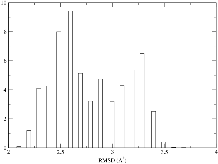
FIG. 1.: Histogram of the sampled root mean squared deviation from native (RMSD in ų at the dimensionless temperature $T=0.6$.) .

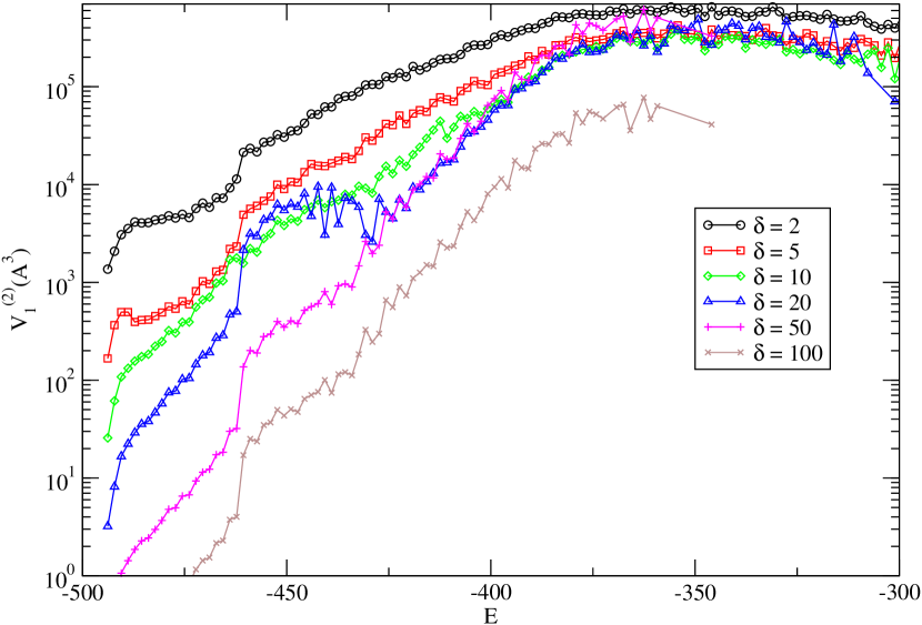
FIG. 2.: Volume of configuration space $V_{1}^{(2)}$ (in ų) that is accessible to rigid translation of chain 2 of the dimer as a function of its energy. Several different choices of the coarse-graining volume $\Gamma_{0}$ are shown in the figure as indicated by the values of $\delta$.

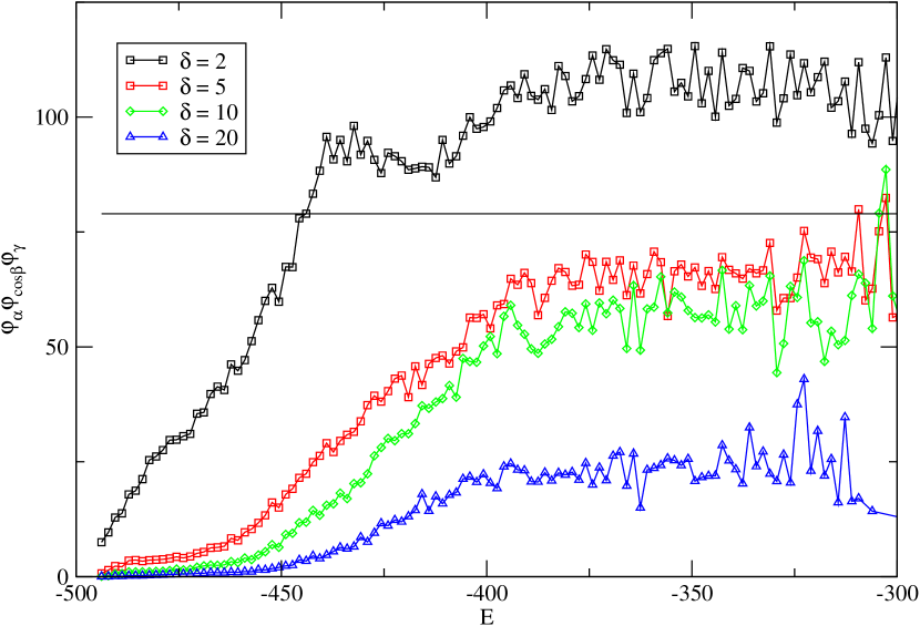
FIG. 3.: Volume of configuration space accessible to rotation of chain 2 of the dimer $\varphi_{\alpha}\varphi_{\cos\beta}\varphi_{\gamma}$ for four different choices of the coarse-graining volume, as indicated by the values of $\delta$ in the figure. The straight line corresponds to the value associated with free rotation, $8\pi^{2}$.

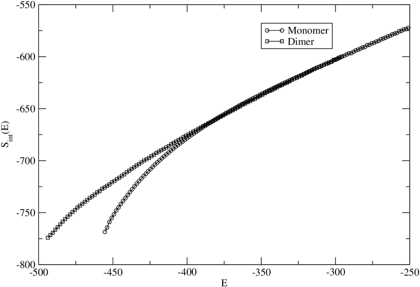
FIG. 4.: Rescaled internal entropy of the dimer $S_{D,int}+S_{0}$, with $S_{0}=52$ (squares), and twice the internal entropy of the monomer $2S_{M,int}(E/2)$ (circles). The value of $S_{0}$ has been graphically determined in order to make the two curves coincide in the range of large $E$. As can be seen from the figure, the two curves superimpose quite accurately for a significant range of energies.

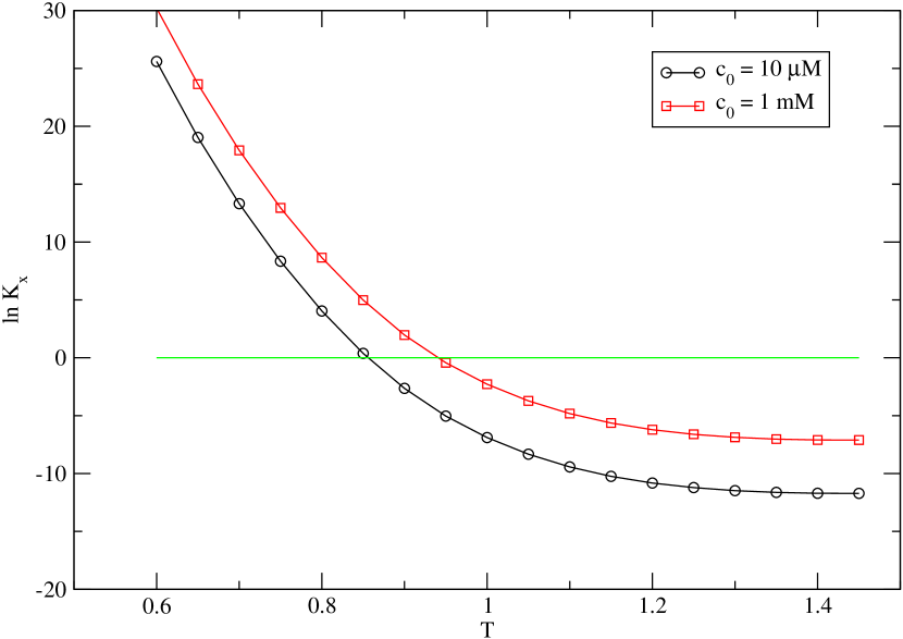
FIG. 5.: Equilibrium reaction constant for monomer-dimer equilibrium as a function of dimensionless temperature and for the two concentrations indicated.

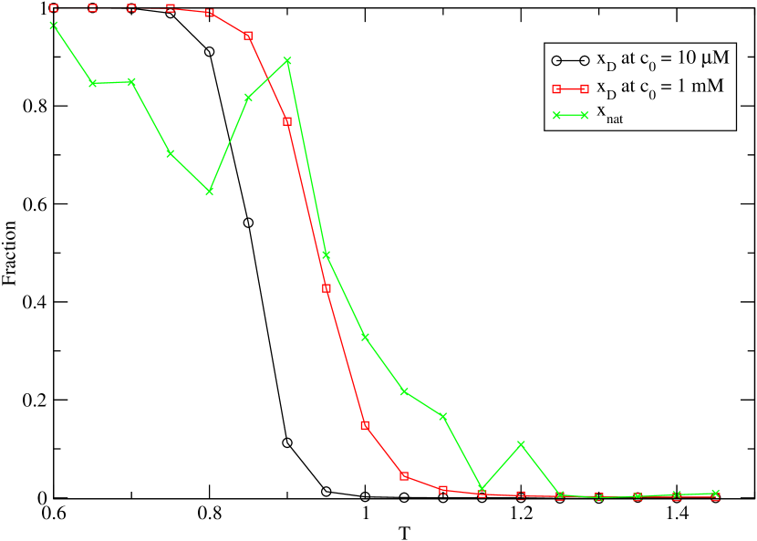
FIG. 6.: Equilibrium mol fraction of the dimer as a function of temperature. $x_{D}=\left(1+4K_{x}-\sqrt{1+8K_{x}}\right)/4K_{x}$, for the two concentrations indicated. The value of the equilibrium constant $K_{x}$ is shown in Fig. 5. We also show the fraction of configurations that, at the given temperature, had at least 50% native contacts.

REFERENCES

- [1] M. Vieth, A. Kolinski, C. Brooks III, and J. Skolnick, J. Mol. Biol. 251, 448 (1995).
- [2] M. Vieth, A. Kolinski, and J. Skolnick, Biochemistry 35, 955 (1996).
- [3] D. Mohanty, A. Kolinski, and J. Skolnick, Biophys. J. 77, 54 (1999).
- [4] F. Crick, Acta Crystallogr. 6, 689 (1953).
- [5] E. O’Shea, J. Klemm, P. Kim, and T. Alber, Science 254, 539 (1991).
- [6] M.-H. Hao and H. Scheraga, J. Chem. Phys. 98, 4940 (1994).
- [7] R. Swendsen and J.-S. Wang, Phys. Rev. Lett. 57, 2607 (1986).
- [8] G. Geyer, Stat. Sci. 7, 437 (1992).
- [9] K. Hukushima and K. Nemoto, J. Phys. Soc. Jpn. 65, 1604 (1996).
- [10] A. Ferrenberg and R. Swendsen, Phys. Rev. Lett. 63-66, 1195 (1989).
- [11] A. Ferrenberg and R. Swendsen, Computers in Physics September/October, 101 (1989).
- [12] A. Kolinski and J. Skolnick, Proteins-Structure, Function, and Genetics 18, 338 (1994).
- [13] A. Kolinski and J. Skolnick, Lattice models of protein folding, dynamics and thermodynamics (R.G. Landes, Austin, 1996).
- [14] F. Bernstein, T. Koetzle, G. Williams, and et al., J. Mol. Biol. 112, 535 (1977).
- [15] A. Kolinski, P. Rotkiewicz, B. Ilkowski, and J. Skolnick, Proteins-Structure, Function, and Genetics 37, 592 (1999).
- [16] A. Kolinski, P. Rotkiewicz, B. Ilkowski, and J. Skolnick, Prog. Theor. Phys. Supp. 138, 292 (2000).
- [17] J. Mayer and M. Goeppert Mayer, Statistical Mechanics (John Wiley & Sons, New York, 1963).
- [18] S.-K. Ma, Statistical Mechanics (World Scientific, Singapore, 1985).
- [19] P. Harbury, T. Zhang, P. Kim, and T. Alber, Science 262, 1401 (1993).
- [20] J. Skolnick, M. Vieth, A. Kolinski, and C. Brooks III, in Modeling of Biomolecular Structures and Mechanisms, edited by A. Pullman et al. (Kluwer Academic, The Netherlands, 1995), p. 95.
- [21] Two residues are considered to be in contact if the distance between the two corresponding particles is smaller than a predefined cut-off. The value of this cut-off distance depends on the pair of aminoacids involved, and has been determined simultaneously with the other parameters that define the interaction potentials. Distances range between approximately 3 and 5 in units of the lattice spacing.
- [22] A. Kolinski and J. Skolnick, Proteins-Structure, Function, and Genetics 32, 475 (1998).