Vector- and tensor-valued descriptors for spatial patterns

Abstract

Higher-rank Minkowski valuations are efficient means for describing the geometry and connectivity of spatial patterns. We show how to extend the framework of the scalar Minkowski valuations to vector- and tensor-valued measures. The versatility of these measures is demonstrated by using simple toy models as well as real data.

0.1 Introduction

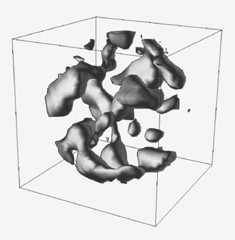
The spatial patterns originating from the polymorphic aggregation of matter in Nature occur on vastly different length scales and with unlimited variety. For instance, the pattern shown in Figure 1 could represent a biological structure obtained with X-ray tomography, or a colloidal cluster in a milky emulsion. In fact, Figure 1 displays an isodensity contour of cosmic matter as traced by the galaxies surrounding the Milky way, which lies in the center of the plot.
The visual impression from such pictures may already convey valuable insight into the dynamic evolution or – in the context of biology – into the functionality of such structures. However, for unbiased inferences

Figure 1: The matter distribution around our galaxy as traced by the PSCz survey. The galaxy number density is smoothed; one isodensity contour is shown (from the PSCz homepage at http://star-www.dur.ac.uk/cosmology/theory/pscz.html).

as well as for the comparison with model simulations, one needs objective and quantitative measures to characterize the geometry and topology of typical structural motifs.
In this article we deal with a family of functions which provide a unique description of the morphology displayed by spatial patterns. We call these functions the Minkowski valuations; they are extensions of the well-known Minkowski functionals often mentioned within this volume (see the contributions by C. Arns et al. and M. Lösche and P. Krüger in this volume as well as beisbart_mecke:additivity in the previous volume LNP 554). Therefore they share some of the simplicity and beauty which the Minkowski functionals own. In particular, they are characterized by simple axioms which set intuitively reasonable standards for a morphological description. In the same way as the Minkowski functionals generalize the notion of the volume, the Minkowski valuations extend the notion of the mass vector (or center of mass) and of the inertia tensor. Like their scalar relatives the majority of the Minkowski valuations are curvature measures integrated over the surface of a pattern.
We start with a short motivation in Section 0.2 by showing that there are good reasons to go beyond the scalar Minkowski functionals. After having outlined ways to generalize the Minkowski functionals (Section 0.3), we review some of the extensions’ mathematical properties in Section 0.4. To illustrate how useful the Minkowski valuations are, we discuss concrete applications covering submolecular up to cosmological scales (Sections 0.5 and 0.6).
Before, two cautionary remarks are appropriate: first, in order to distinguish conceptually between the scalar Minkowski functionals and their higher-rank extensions, we shall address the whole entirety of Minkowski functionals and their extensions via the term “Minkowski valuations” (MVs), whereas “Minkowski functionals” (MFs) is reserved to the scalar Minkowski functionals as before. Secondly, there is a vivid theoretical development of higher-rank Minkowski valuations these days beisbart_schneider:tensor ; beisbart_schneider:tensor2 ; beisbart_beisbart:tensor . Therefore, this overview can not provide a complete survey on Minkowski valuations; on the contrary, substantial progress is to be expected both from the mathematical side as well as from applications. For instance, morphological analysis based on Minkowski valuations may be useful to quantify molecular orientations (see the contributions by F. Schmid and N. H. Phuong, U. S. Schwarz and G. Gompper, D. Jeulin, C. Arns et al., and H.-J. Vogel in this volume). Our vector-valued descriptors may also be used to refine the morphological analysis of Langmuir monolayer phases (presented by M. Lösche and P. Krüger in this volume) which has so far been based merely on scalar MFs. Another application may cover the geometric characterization of liquid foams described by F. Graner in this volume, where stress tensors need to be related to a complex spatial structure.

0.2 Going beyond scalar Minkowski functionals – a physical motivation

The following problem is typical for challenges occurring in physics: the formation of galaxy clusters depends in a complicated way on the background cosmology usually described in terms of a cosmological model. Such a model is defined through the values of the cosmological parameters and the power spectrum of the initial density perturbations beisbart_peebles:principles ; beisbart_bartelmann:arcIV . In order to investigate the impact of the background cosmology on galaxy clusters one carries out gravitational $N$-body simulations; typical results comprise cluster images such as those shown in Figure 2. To compare the models and to check which model fits best present-day cluster observations, one has to use quantitative and discriminative morphological measures.

Figure 2: The projected matter distribution of two simulated galaxy clusters (from the GIF-project). Their different morphologies are due to different values of the cosmological parameters and to different initial power spectra imposed (left panel: $\tau$ Cold Dark Matter model; right panel open Cold Dark Matter model, see beisbart_bartelmann:arcIV for more details). Apart from that, however, the clusters stem from comparable initial conditions. In order to distinguish between both models we need a thorough morphological description.

The Minkowski functionals certainly place practical tools at the physicist’s disposal. Defined on the convex ring ${\mathcal{K}}_{d}$, i.e. for finite unions of compact, convex sets in $d$-dimensional Euclidean space, they are the only motion-invariant, convex-continuous, and additive descriptors. Despite this very general characterization there are only a finite number of Minkowski functionals, namely $(d+1)$ in $d$ dimensions (characterization theorem, beisbart_hadwiger:vorlesung ; beisbart_klain:hadwiger ). They have simple geometrical meanings derived from their representation as integrals. These integrals either extend over the pattern itself to yield the volume, or cover its surface which is weighted with combinations of the local curvatures in order to give – in two dimensions, e.g. – the perimeter and the integrated curvature (which equals the Euler characteristic). The Minkowski functionals also arise quite naturally as expansion coefficients in the Steiner formula beisbart_schneider:brunn specifying the volume of the parallel body of a convex body. Indeed, the Minkowski functionals have been extensively applied to physical structures at vastly different length scales, see beisbart_mecke:additivity for an overview and beisbart_kerscher:statistical for astrophysical applications. On the mathematical side, numerous useful results such as the principal kinematic formulae or the Crofton formulae (see beisbart_hadwiger:vorlesung ) have been proven with integral geometric methods.
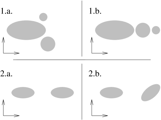
However, the morphometry with Minkowski functionals is by no means comprehensive. Combining two of their defining principles, additivity and homogeneity, one can easily see, that, e.g., moving a connected part of a pattern results in significant visible changes which can not be detected by the Minkowski functionals at all. This is illustrated in the first panel of Figure 3 representing schematic clusters. It is surely of interest, however, in which way the subclumps of a system are arranged, and how they are aligned with respect to each other (see the second panel of Figure 3). Therefore, we have to move beyond the scalar Minkowski functionals. It turns out that one can generalize the Minkowski functionals without leaving the mathematical framework of integral geometry.

Figure 3: Neither the schematic clusters displayed in panel 1.a. and 1.b. nor both patterns in panel 2.a. and 2.b. can be distinguished from each other using only the scalar Minkowski functionals. Additivity and motion-invariance prevent the MFs from discriminating between the different positions (upper panels) or different orientations (lower panels) of the subcomponents, respectively.

0.3 The hierarchy of Minkowski valuations – extending the framework

There are several ways to extend the framework of the Minkowski functionals. For instance, one may start with Steiner’s formula.

The Steiner formula.

It is a natural choice to employ the volume $V(K)=\int_{K}{\rm d}V$ of a body $K$ for its very coarse description. If the parallel body $K_{\epsilon}$ is considered, which contains all points closer to $K$ than $\epsilon>0$, and if $K$ is convex, then one finds from Steiner’s formula an expansion for $V(K_{\epsilon})$ in powers of $\epsilon$,

$$V\left(K_{\epsilon}\right)=\sum_{\nu=0}^{d}\binom{d}{\nu}\epsilon^{\nu}W_{\nu}\;\;\;,$$ (1)

where the Minkowski functionals $W_{\nu}$ arise as expansion coefficients. The latter functionals are useful morphometric concepts and can be extended to non-convex patterns. In this sense, the volume quite generally leads to a family of related measures.
Since we saw that in some applications (recall the upper panels of Figure 3) the position of a body may be worth considering, we specify the location of $K$ with its mass vector

$$V^{1}\left(K\right)\equiv\int_{K}{\rm d}V{\mathbf{x}}\;\;\;.$$ (2)

Alternatively, we could introduce its center of mass ${\mathbf{p}}_{0}\equiv V^{1}/V$.
Moreover, as the lower panels of Figure 3 indicate, the body’s orientation may be relevant. In this case we have to move on to even higher moments; for instance, the tensor

$$V^{2}\left(K\right)\equiv\int_{K}{\rm d}V{\mathbf{x}}{\mathbf{x}}$$ (3)

(where ${\mathbf{x}}{\mathbf{x}}$ denotes the symmetric tensor product) contains information on main directions of the body $K$. Note, that both the mass vector of a body and its inertia tensor (the traceless part of Equation 3: $V^{2}(K)-{\rm Tr}\left(V^{2}(K)\right)E_{d}$, where $E_{d}$ is the $d$-dimensional second-rank unit tensor) are of major interest for the physicist: the mass center of a rigid body moves in space as if the whole force acting on the body was concentrated onto a point particle at its center of mass. The inertia tensor determines how a body is rotating, given a fixed angular momentum. – Higher-rank moments such as symmetric $r$-rank tensors of the form $V^{r}\left(K\right)\equiv\int{\rm d}V{\mathbf{x}}^{r}$ with $r>2$, may be considered, too.
Now it is again possible to write down a Steiner-type formula for the transition to the parallel body of a convex set $K$ beisbart_schneider:schwerpunkte ; beisbart_schneider:tensor : the scalar expansion coefficients have to be replaced by vector- or tensor-valued coefficients. The following simple argument shows that not only the character, but also the number of coefficients has to change: for a unit ball centered at the origin, $B_{R}(0)\equiv\big{\{}{\mathbf{x}}\big{|}|{\mathbf{x}}|\leq R\big{\}}$, the construction of the parallel body results in $B_{(\epsilon+R)}(0)$. On the other hand, as a simple calculation shows, $V^{r}\left(B_{(\epsilon+R)}({\mathbf{x}})\right)\propto\left(\epsilon+R\right)^{d+r}$. Thus, powers up to $(d+r)$ arise in the generalization of Steiner’s formula, which we write formally as

$$V^{r}\left(K_{\epsilon}\right)=\sum_{\nu=0}^{d+r}\epsilon^{\nu}M_{r,\nu}\;\;\;.$$ (4)

As for the scalar Minkowski functionals, one can obtain an integral representation of the Steiner coefficients by considering a smooth and convex body $K$.

Figure 4: The fact that each volume element in $K$ is weighted with the position vector in order to give $V^{r}(K)$ for $r>0$, makes the local normal ${\mathbf{n}}$ relevant for the parallel body $K_{\epsilon}$.

From the integral representation of the scalar MFs and from the form of the moments $V^{r}$ one might guess that the coefficients $M_{r,\nu}$ are built by functions of the form:

$$\int_{\partial K}{\rm d}S^{d-1}{\mathbf{x}}^{r}s_{\nu}\left(\kappa_{1},..,\kappa_{d-1}\right)$$ (5)

with the elementary symmetric functions $s_{\nu}$ for $\nu=0,..,(d-1)$ of the local curvatures $\kappa_{1},..,\kappa_{d-1}$ (for a definition, see beisbart_schneider:tensor ). But this will not suffice, since we need $(d+r)$ coefficients. A closer look shows (see Figure 4), that indeed the local normal vector comes into play; for, if ${\mathbf{x}}\subset\partial K$, then ${\mathbf{x}}+\epsilon{\mathbf{n}}$ lies on the surface of $K_{\epsilon}$; here ${\mathbf{n}}$ denotes the local normal vector to $\partial K$ at the point ${\mathbf{x}}$. The weighting with the local position in the definition of $V^{r}$ therefore leads to contributions from local normal vectors in the Steiner formula. In beisbart_schneider:tensor it is shown that in general the expansion coefficients $M_{r,\nu}$ can be written as linear combinations of the quantities:

$$W_{\nu}^{p,q}\equiv\frac{1}{\nu\binom{d}{\nu}}\int_{\partial K}{\rm d}S^{d-1}s_{\nu-1}\left(\kappa_{1},..,\kappa_{d-1}\right){\mathbf{x}}^{p}{\mathbf{n}}^{q}$$ (6)

for $\nu=1,..,d$, and $p,q\in{\mathbb{N}}_{0}$. Now the $W_{\nu}^{p,q}$ look more basic than the coefficients arising in the Steiner formula for the volume tensor. It seems therefore, as if, in contrast to the case of the scalars, the Steiner coefficients are no longer the basic quantities. In order to generalize the Minkowski functionals we therefore have to move to an alternative route.

Spatial moments of the Minkowski functionals.

Let us take the moments $V^{r}$ together with the $W_{\nu}^{r,s}$ ($\nu=0,..,(d-1)$, $r,s=0,1,..$) as basic quantities. In order to arrive at a coherent notation, we set $W^{r,0}_{0}\equiv V^{r}$ and $W^{r,j}_{0}=0$ for $j>0$. Higher-rank Minkowski functionals therefore are higher moments of the scalar Minkowski functionals where the local surface is weighted with both position and surface normal. If the body $K$ is shifted with a translation vector ${\mathbf{t}}$, then the $W_{\nu}^{r,s}$ transform like

$$W_{\nu}^{r,s}\left(K+{\mathbf{t}}\right)=\sum_{p=0}^{r}W_{\nu}^{p,j}{\mathbf{t}}^{i-p}\binom{i}{p}\;\;\;,$$ (7)

as follows immediately from their definition. For rotations $R$, we have

$$W_{\nu}^{r,s}\left(RK\right)=RW_{\nu}^{r,s}\left(K\right)\;\;\;,$$ (8)

where we use the fact that the $d$-dimensional orthogonal group $O(d)$ has a natural representation in each tensor space.
Recalling that the Minkowski functionals can be described axiomatically, one would be inclined at this point to look for a characterization theorem for vectors and tensors. It turns out that one has to include even more valuations in order to achieve that purpose.

Axiomatic characterization.

A rigorous way to extend the Minkowski functionals is therefore to relax one of their defining axioms. We keep the additivity

$$\Phi(A\cup B)=\Phi(A)+\Phi(B)-\Phi(A\cap B)$$ (9)

for a tensor valuation $\Phi$; we also maintain the conditional continuity, i.e. continuity for the subclass of convex bodies; but, in the spirit of our previous findings, we replace the motion invariance by motion covariance defined as follows: for translations we require the existence of a number $n\in{\mathbb{N}}_{0}$ and of functions $\Phi_{i}$ ($i=0,..,n$) such that for all $K$

$$\Phi(K+{\mathbf{t}})=\sum_{i=0}^{n}\Phi_{i}(K){\mathbf{t}}^{i}\;\;\;.$$ (10)

Note, that products such as $\Phi_{i}(K){\mathbf{t}}^{i}$ always denote symmetric tensor products. For rotations we use the natural representation of $O(d)$ in the space of tensors as before, and require for $R\in O(d)$:

$$\Phi(RK)=R\Phi(K)\;\;\;.$$ (11)

In a seminal work, Alesker beisbart_alesker:tensor proved the following characterization theorem: every motion-covariant, convex-continuous, and additive mapping $\Phi$ can be written as a linear combination of the functionals

$$E_{d}^{k}W_{\nu}^{r,s}$$ (12)

with $i,j,k\in{\mathbb{N}}_{0}$ and $\nu=0,..,d$. $E_{d}$ denotes the $d$-dimensional unit matrix.
Equation (12) gives all of the Minkowski valuations and finally answers the question how to generalize the MFs in a suitable manner. It contains more valuations than those given in Equation (6). However, some caution has to be exercised: Alesker’s theorem beisbart_alesker:tensor only bounds the dimension of the tensor functional spaces from above. It is not obvious that all of the above functionals are linear independent. Indeed, beisbart_mcmullen:tensor proved some linear relationships holding among the tensors. In order to give one example, Gauß’ theorem yields

$$W_{1}^{1,1}=\int_{\partial K}{\rm d}S^{d-1}{\mathbf{x}}{\mathbf{n}}=W_{0}^{0,0}(K)E_{d}\;\;\;.$$ (13)

One therefore has to explore the different tensor ranks further.

0.4 Exploring higher-rank Minkowski valuations

0.4.1 Some mathematical results

Minkowski vectors.

Minkowski vectors, i.e. Minkowski valuations of rank one, have been known for some years beisbart_hadwiger:vekt ; beisbart_schneider:schwerpunkte ; beisbart_schneider:schwerpunkte2 ; beisbart_hadwiger:vect2 . There is a strict one-to-one correspondence between the vectors and the scalars: for each Minkowski functional $W_{\nu}\propto\int_{\partial K}s_{\nu-1}\left(\kappa_{1},..,\kappa_{d-1}\right)$ there is a related vector $\int_{\partial K}s_{\nu-1}\left(\kappa_{1},..,\kappa_{d-1}\right){\mathbf{x}}$, such that $(d+1)$ vectors exist altogether. The reason why no normals enter at this level is basically because for compact convex bodies $\int_{\partial K}s_{\nu-1}\left(\kappa_{1},..,\kappa_{d-1}\right){\mathbf{n}}=0$  for $\nu=0,..,(d-1)$ (for an elementary proof see beisbart_hadwiger:vect2 ). The integral geometry of vectors was extensively scrutinized, see, e.g., beisbart_hadwiger:vekt . For physical applications of vectors (see beisbart_beisbart:querletter ; beisbart_beisbart:fp ) the curvature centroids

$${\mathbf{p}}_{i}\equiv W_{\nu}^{1,0}/W_{\nu}^{0,0}\quad{\rm(}\nu=0,..,d{\rm)}$$ (14)

are a useful concept. Their meaning is straight forward: they locate morphological information. We shall see below that, if the curvature centroids do not coincide within one point, strong evidence for asymmetry is given.

Second-rank tensors.

The situation becomes more complicated for higher-rank tensors. It can be shown, that at the second rank, the following $(3d+1)$ tensors provide a base beisbart_beisbart:tensor :

$$\int_{K}{\rm d}V{\mathbf{x}}{\mathbf{x}}\;\;\;,$$ (15)

$$\int_{\partial K}{\rm d}S^{d-1}s_{\nu}{\mathbf{x}}{\mathbf{x}}\;\;\;,\quad\int_{\partial K}{\rm d}S^{d-1}s_{\nu}{\mathbf{x}}{\mathbf{n}}\;\;\;,\quad\int_{\partial K}{\rm d}S^{d-1}s_{\nu}{\mathbf{n}}{\mathbf{n}}$$ (16)

for $\nu=0,..,(d-1)$. Not all of them are interesting from a physical point of view, since some of them are related to Minkowski functionals times the unit tensor and thus do not contain any new information. Principal kinematic formulae and Crofton formulae are known for second-rank tensors beisbart_schneider:tensor ; beisbart_beisbart:tensor ; beisbart_schneider:tensor2 .
For a geometrical interpretation, we have to bear in mind, that the values of the tensors depend on the origin adopted. For $W_{\nu}^{2,0}$ ($\nu=0,..,d$), however, the corresponding curvature centroid ${\mathbf{p}}_{\nu}$ is a natural reference point; the other tensors listed in Equation (16) are translation-invariant. Obviously, with such a choice the tensors are sensitive to morphological anisotropies, in the case of symmetry they align along the symmetry axes, otherwise they distinguish morphologically interesting directions. It is therefore useful to consider their eigenvalues and eigendirections.

Beyond second rank.

Although higher-rank tensors may be interesting as well, we shall not consider them further at this point.

0.4.2 Examples

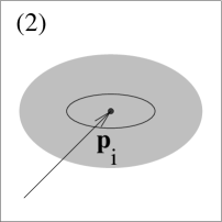
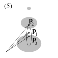
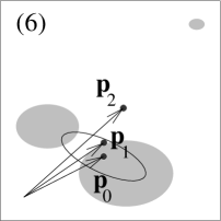
In order to give a first example of how the Minkowski valuations discriminate spatial structures, we consider a few simple patterns as shown in Figure 5.

Figure 5: A number of simple patterns together with their curvature centroids ${\mathbf{p}}_{i}$ ($i=0,..,2$). The ellipse represents the mass tensor $W_{0}^{2,0}/W_{0}^{0,0}$; it is calculated with the center of mass ${\mathbf{p}}_{0}$ as reference point. The ellipses indicate the ratio of the eigenvalues and the eigendirections as well.

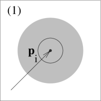
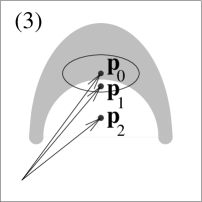
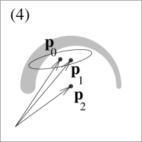
In the case of a circle (panel 1) the curvature centroids coincide within the circle’s center; the tensors – here represented as an ellipse featuring their eigenvalues and the corresponding directions – are isotropic. It is useful to divide the tensors $W_{\nu}^{r,s}$ by the corresponding Minkowski functionals $W_{\nu}^{0,0}$. The trace of the normalized tensor (i.e. the sum of the eigenvalues) quantifies to which extent the morphological information is concentrated around the center, how large the morphological fluctuations around the center are.
The transition to an ellipse of the same volume as the circle (panel 2) can be traced either with the tensors becoming anisotropic or with the ratio of the squared surface to the volume (isoperimetric ratio, see beisbart_schmalzing:webI ). Furthermore, as the morphological concentration is decreasing, the traces of most of the normalized tensors increase, especially of $W_{2}^{2,0}$: the more elongated the ellipse becomes, the higher is its curvature at its very fringes along the horizontal direction. The normalized trace of $W_{1}^{1,1}$, on the contrary, becomes smaller, since the normal and the local position vector cease to be parallel to each other. The curvature centroids still coincide with each other because of the point symmetry. – If we reduce the symmetry further to a merely axially symmetric configuration (panel 3), the curvature centroids fan out along the symmetry axis. In the case of no symmetry at all (panel 4) they may constitute a triangle.
Finally, suppose one is given three convex bodies (or $d+1$ ones in $d$ dimensions) with known Minkowski functionals in order to combine them into a pattern such as indicated in panels 5 and 6. Given the scalar measures of the whole pattern, especially its Euler characteristic, one can constrain the number of intersections or subclumps in a pattern, which does not make any difference in our examples. For disentangling the positions of the grains, however, one has to know the curvature centroids. The centroids weight the subclusters according to their Minkowski functionals. Therefore, whereas from the volume’s point of view, only the larger components contribute significantly, all subclumps have the same weight (Euler characteristic $=1$) for the curvature centroid ${\mathbf{p}}_{2}$. If the subclumps do not overlap, one can indeed completely recover their positions.
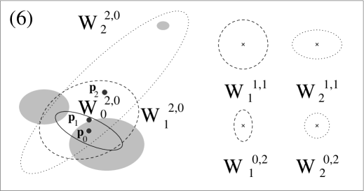
In Figure 6, we show all tensors for the last example in more detail. Obviously, there are not only anisotropies; rather different morphological directions are relevant. The volume concentration around the center of mass is relatively high, since the volume is dominated by the two largest subclusters, being close to each other. It is quite the opposite with $W_{2}^{2,0}$: ${\mathbf{p}}_{2}$ is relatively far away from all the clumps, the curvature around ${\mathbf{p}}_{2}$ is dispersed leading to a high value of tensor’s trace. The main relevant direction connects the pair of large clumps with the third subcluster. The tensor $W_{1}^{1,1}$ is always isotropic, as shown in Equation (13), its trace is connected to the volume. Obviously, $W_{2}^{1,1}$ and $W_{1}^{0,2}$ complement each other; indeed they add up to a diagonal tensor (recall the linear relationships described in beisbart_schneider:tensor ). Their eigenvectors’ alignment with the coordinate axes is due to the fact that all the subclumps are aligned parallel to the axes as well. Otherwise, $W_{2}^{1,1}$ and $W_{1}^{0,2}$ would average over the orientations of the subclumps. Finally, $W_{2}^{0,2}$ is isotropic, its trace equals the Euler characteristic.
The detailed description of patterns given by the Minkowski valuations can be used in practical applications, as we shall see in the next section.

Figure 6: We show all of the tensors $W_{0}^{2,0}$, $W_{\nu}^{2,0}$, $W_{\nu}^{1,1}$, and $W_{\nu}^{0,2}$ for $\nu=1,2$ – they span a base of the second-rank tensor space. The tensors $W_{\nu}^{r,s}$ were divided by $W_{\nu}^{0,0}$ ($i=0,..,2$); the tenors with a twofold position weighting ($W_{\nu}^{2,0}$) are calculated around the corresponding centroid. All of the other tensors are translation-invariant. Therefore we depict them outside the pattern on the right-hand-side. Their eigenvalues are multiplied by a factor of $6$ in order to yield a more convenient representation. $W^{2,0}_{0}$: solid line; $W^{2,0}_{1}$, $W^{1,1}_{1}$, $W^{0,2}_{1}$: dashed line; $W^{2,0}_{2}$, $W^{1,1}_{2}$, $W^{0,2}_{2}$: dotted line.

0.5 Physical applications of higher-rank Minkowski valuations

0.5.1 The inner structure of spiral galaxies

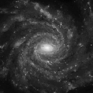
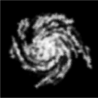
The classification of spiral or disc galaxies into specific types (the Hubble types, e.g., beisbart_hubble:classification ) is an important step towards their physical understanding; there are competing theoretical pictures trying to explain the formation of spiral arms beisbart_lin:spiral ; beisbart_gerola:stochastic . In Figure 7 we display a real galaxy observed face-on together with a simulation according to a percolation model beisbart_gerola:stochastic . So far one has mainly relied on an assignment by eye in order to classify observed disc galaxies and to compare observational data with theoretical models beisbart_naim:comparative . One of the reasons for this is that spiral arms are easily detected by the human eye, but are rather hard to quantify. Here we use Minkowski valuations to reveal aspects of the inner structure of spiral galaxies (see beisbart_russell:spiral ; beisbart_block:spiral ; beisbart_kornreich:asymmetry for some discussion of how to quantify morphometric features of spiral galaxies, and especially beisbart_abraham:automated ; beisbart_abraham:asymmetry ).
In order to render an optical galaxy image accessible to a Minkowski analysis, it is helpful to understand it as a two-dimensional surface brightness field $u({\mathbf{x}})$. We may then estimate the Minkowski valuations of the excursion sets $M_{v}=\{{\mathbf{x}}|u({\mathbf{x}})>v\}$. Contrary to large scale cosmological data (e.g. the distribution of galaxies or clusters of galaxies), such a density field is neither homogeneous nor isotropic; rather it reveals a point of considerable symmetry: the center of mass. We expect the curvature centroids to coincide within this point and therefore concentrate on second-rank Minkowski tensors.

Figure 7: The spiral galaxy NGC 1232 (as observed by the VLT/ESO) and a simulated galaxy following the model by beisbart_seiden:percolation .

In order to detect a possible overall anisotropy, we divide the smaller eigenvalue of $W^{2,0}_{0}$ by the larger one; this yields the parameter $X$. Since $X\leq 1$ by definition, $\epsilon\equiv 1-X$ can serve as a measure of the anisotropy. Such an anisotropy may reflect a physical anisotropy, induced, for instance, by the presence of two massive spiral arms, but may also indicate that the galaxy is not observed face on, but rather under an inclination angle.
As the tensors $W^{2,0}_{\nu}$ ($\nu=0,..,2$) weight the volume or the surface, respectively, with ${\mathbf{x}}{\mathbf{x}}$, their eigenvalues are increased, if the configuration is more widespread (see Fig. 8). This fact can be used to quantify the concentration of a density field around its center of mass, by calculating the trace of $W^{2,0}_{\nu}$.

Figure 8: The tensors $W^{2,0}_{0}$ (solid line) and $W^{2,0}_{1}$ (dashed line) for a wide spread (right panel) and a compact (left panel) configuration of circles. The eigenvalues depend quadratically on the separation of the circles.

Therefore another characteristic feature of disc galaxies, namely the way in which the radial surface brightness distribution declines (with increasing radius), can be analyzed by scanning through various threshold values $v$. We applied (suitably normalized) concentration parameters $P_{\nu}$ (built from ${\rm Tr}(W^{2,0}_{\nu})$) to the images of both real galaxies (C. Moellenhoff, private communication) as well as to galaxies produced by a percolation model (beisbart_seiden:percolation ; see beisbart_dahlke:diploma for details). These morphological descriptors reveal strong luminosity concentration for real galaxies, which could not be reproduced by any of the model galaxies (see Fig.9) with reasonable choices for the model parameters. Using the morphology of observed disc galaxies, one can therefore rule out the percolation model (at least in its simple form) as a viable attempt to explain the formation of spiral arms.

Figure 9: Results of a quantitative morphometry for spiral galaxies using Minkowski tensors. We consider the galaxy NGC 1232 (shown in the left panel of Figure 7) and a sample of model galaxies following a percolation model (an example of a model prediction is displayed in the right panel of Figure 7). We plot two concentration parameters (as described in the main text) versus decreasing surface brightness threshold values, i.e. increasing surface area. The error bars indicate $1\sigma$ fluctuations around the expectation value of the model, whereas the single line refers to NGC 1232. The parameter C_A reveals significant differences in the concentration between the surface brightness profiles of real and model galaxies. The particular percolation model used thus is incompatible with real data.

0.5.2 The morphology of galaxy clusters

As mentioned in Section 0.2, the morphology of clusters may constrain the values of the cosmological parameters. Intuitively, one may expect clusters in cosmological low-density models to have less substructure than in high-density models beisbart_richstone:cluster . Using Minkowski valuations, we check whether this effect can be observed for the cosmological GIF simulations beisbart_bartelmann:arcIV . We analyze the clusters’ projected mass distributions such as shown in Figure 2. Observations from the gravitational lensing through clusters beisbart_schneider:book ; beisbart_fischer:lens trace approximately the same cluster information.
In order to make the simulation data, which consist of “particles tracing matter”, accessible to the Minkowski valuations, we construct a pixelized density field $u({\mathbf{x}})$ and smooth it with a Gaussian kernel of width $\lambda=0.3{{h^{-1}{\rm Mpc}}}$. The resulting field $u_{\lambda}({\mathbf{x}})$ contains the overall shape of the cluster. Again we estimate the Minkowski valuations of the excursion sets, which contain all pixels above a given density threshold $v$. Our method to estimate the Minkowski functionals from the grid is based upon Crofton’s formulae beisbart_serra:morphology ; beisbart_schmalzing:beyond ; beisbart_beisbart:diss . For each cluster we average a function of the Minkowski valuations $f$ over different density thresholds:

$$\frac{1}{\left(u_{\lambda}\right)_{2}-\left(u_{\lambda}\right)_{1}}\langle f\rangle\equiv\int_{\left(u_{\lambda}\right)_{1}}^{\left(u_{\lambda}\right)_{2}}{\rm d}u_{\lambda}f$$ (17)

in order to obtain a compact set of parameters. Here $\left(u_{\lambda}\right)_{1}$ and $\left(u_{\lambda}\right)_{2}$ denote appropriately chosen integration limits. We consider five types of substructure.

1. The clumpiness C $\equiv\sqrt{\langle\left(\frac{1}{\pi}W_{2}-1\right)^{2}\rangle}$ counts the number of subclumps in quantifying how much the Euler characteristic $W_{2}/\pi$ deviates from one.

2. The construction of the asymmetry parameter A is based on the fact that curvature centroids which do not coincide with each other, indicate asymmetry. Therefore, we calculate the perimeter of the triangle constituted by the curvature centroids, $2W_{1}\left(\Delta\left({\mathbf{p}}_{i}\right)\right)$, A$\equiv\langle W_{1}\left(\Delta\left({\mathbf{p}}_{i}\right)\right)\rangle$.

3. The ratio of the tensors’ eigenvalues, $\gamma_{1}\left(W_{\nu}^{r,s}\right)/\gamma_{2}\left(W_{\nu}^{r,s}\right)$ tells us to which extent anisotropies are present. Here we consider the tensor $W_{1}^{2,0}$ and define X$\equiv\Big{\langle}\gamma_{1}\left(W_{1}^{2,0}\right)/\gamma_{2}\left(W_{1}^{2,0}\right)\Big{\rangle}$.

4. In general the curvature centroids ${\mathbf{p}}_{\nu}$ wander in space if the density threshold is varied; their fluctuations therefore measure the shift of morphological properties. Focusing on ${\mathbf{p}}_{1}$ we define S$\equiv\langle\left({\mathbf{p}}_{1}-\langle{\mathbf{p}}_{1}\rangle\right)^{2}\rangle$. This parameter is related to the centroid variation used in cluster investigations beforebeisbart_mohr:x-ray-cluster .

5. Likewise, the eigendirections (parametrized by an angle $\alpha$) of the tensors are changing; this generates the twist of morphological properties. Restricting ourselves to $W_{1}^{2,0}$ we employ the parameter T$\equiv\langle\left(\alpha-\langle\alpha\rangle\right)^{2}\rangle$.

For more technical details, see beisbart_beisbart:diss .

Figure 10: The average morphological evolution of galaxy clusters from the GIF simulations. Our morphological order parameters clumpiness C, asymmetry A, anisotropy X, shift of morphology S and twist of morphology T are shown versus time. The time is given in terms of the observable cosmological redshift. Redshift $z=0$ means the present day, higher redshifts lead back into past. In order to get typical results for two cosmological models (low-density model with an open geometry, called open Cold Dark Matter, OCDM: dashed line; high-density model with a massive $\tau$ neutrino, named $\tau$CDM: solid line) we average over about $15$ clusters and $3$ orthogonal projections per cluster within each model. As the results show, our morphological order parameters quantitatively feature the differences between the models which are in accordance with the theoretical predictions. For details on the cosmological Cold Dark Matter models see beisbart_peacock:cosmological

For each time period (or cosmological redshift) we estimate the order parameters for three projections per cluster and average over all clusters in one cosmological model in order to extract a typical morphology. In Figure 10, we display the evolution of the averaged morphological parameters vs. redshift. One recognizes immediately a relaxation process, leading to less substructure (and lower values of the morphological order parameters) as time goes by (from right to left). Furthermore, clear differences between the cosmological background models arise. Indeed the theoretical predictions according to which the low-density clusters (OCDM) exhibit less substructure, are confirmed for the past; for redshift $z=0$, the differences disappear.
All of our order parameters show a similar behavior. The reason probably is that we average over different types of relaxation processes. An investigation of single clusters should reveal differences between, e.g., a bimodal merger dominated by two colliding subclumps and a more isotropic mass infall.

0.5.3 The geometry of the electric charge distribution in molecules

An important implication of the atom hypothesis is that the structures of molecules are to be explained in terms of their constituent parts, the atoms. Heuristic principles based upon this assumption work quite well in chemistry. However, if one tries to justify this hypothesis in the framework of quantum mechanics, the notion of an individual atom seems to disappear, since the negative charge distributions of the atoms merge, blurring the electron clouds which define the single atoms.
Bader beisbart_bader:quantum proposed an elegant method to recover the notion of atoms in molecules. Since, from the quantum mechanical point of view, the charge density profile $\varrho({\mathbf{r}})$ is the only relevant quantity, its geometry and topology must contain the notion of atoms. Using the critical points of the density distribution $\varrho$, where $\nabla\varrho=0$, one can define atoms as local density maxima together with a surrounding domain enclosed by zero-flux surfaces. This geometrical approach can be extended to chemical bonds and has been justified on physical grounds. 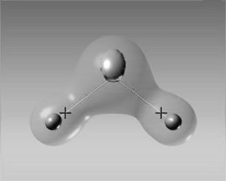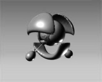Moreover, it provides us with means to visualize molecules in a proper way using the charge density profile, see Figure 11 for an illustration. A distinguished role is played by the surface $\nabla^{2}\varrho=0$ which separates the zone where chemical reactions are likely to happen from the rest of space.

Figure 11: The water molecule H₂O. The bright lines denote the bonds connecting the H-atom with both of the O-atoms. The crosses mark the points where the zero-flux surfaces separating the atoms intersect with the bonds. Moreover, some iso-surfaces of the Laplacian of the charge density, $\triangle\varrho$, are shown. The images are from http://www.nas.nasa.gov/$\sim$creon/papers/mgms96/ (courtesy C. Levit). The panels show different projections and focus on different iso-surfaces.

Obviously, this is an area of research where physics and geometry strongly interact, and the applications of higher-rank Minkowski valuations may yield useful information on the structure of the chemical bonding. First, the morphology of the whole molecules can be simply described in terms of the Minkowski valuations of the density field. The atoms, which Bader defines beisbart_bader:quantum , may not be compact in every case, so the single atoms can not be understood in terms of the Minkowski valuations. However, the fact that the atoms’ positions are specified in Bader’s theory gives us the chance of probing the molecular structure with the Boolean grain method where the atoms’ positions are decorated using spheres (either monodisperse or with radii mirroring physical quantities). Note, that at this point one really needs tensors, since in this case the locations and the orientations of subsystems are of crucial importance; and this local information lies beyond the scope of the scalar measures. Bader’s theory constructs also a graph of bonds, that may be analyzed with Minkowski valuations straightfowardly.
But given the fact that both the molecules and the constituting atoms are defined in terms of geometry, one may go one step further and try to discover phenomenological principles allowing one to predict the shape of molecules given their constituents.
These endeavors clearly are beyond the scope of this article. However, in order to illustrate to some extent how useful the Minkowski valuations may prove in this area, we consider briefly some of the Minkowski tensors for the H${}_{2}^{+}$ ion.

Figure 12: The morphology of the bonding and the anti-bonding states of the electron within the $H^{+}_{2}$ ion. We explore the charge distribution of the electron via the Minkowski tensors of excursion sets from the density field. In the left panel, we show the trace of $W^{2,0}_{1}$ as a function of the charge fraction q enclosed within the density contour. In the right panel, we consider the anisotropy of the charge distribution. It is quantified via $An\equiv\left(\left(W^{2,0}_{1}\right)_{xx}-\left(W^{2,0}_{1}\right)_{yy}\right)/{\rm Tr}\left(W^{2,0}_{1}\right)$. The anti-bonding state, shown as the dashed line is much more anisotropic than the bonding state which wraps both atoms with a smooth electron hull.

In order to treat the H${}_{2}^{+}$ ion consisting of two protons and an electron in the framework of quantum mechanics, one often considers the protons as fixed in space (Born-Oppenheimer approximation) thereby reducing the problem to an effective one-particle problem of an electron moving in the potential of two positively charged nuclei. A reasonable ansatz for the quantal wave function of the electron – at least suitable to illustrate what is basically happening – is a superposition of quantum states where the electron is bound to either of the protons. To be more precise, let us consider the protons as being separated by their equilibrium distance of approximately two Bohr radii. Let us label the protons with $1$ and $2$ and let $\psi_{i}$ denote the unperturbed (well-known) hydrogen ground state wave function of an electron bound to proton $i$ for $i=1,2$. For symmetry reasons, only the linear combinations

$$\psi_{a}=\frac{1}{\sqrt{2}}\left(\psi_{1}-\psi_{2}\right)\quad{\rm and}\quad\psi_{b}=\frac{1}{\sqrt{2}}\left(\psi_{1}+\psi_{2}\right)$$ (18)

are of interest. Since $\psi_{b}$ is favored on energetic grounds, it is a bonding state; consequently $\psi_{a}$ is called antibonding state.
The morphology of the electron charge distribution is expected to distinguish between both states. Let us consider excursion sets of the three-dimensional electron charge density profile $\varrho=|\psi|^{2}$ for both states. In Figure 12 we display the surface tensor $W_{1}^{2,0}$ as a function of the charge fraction enclosed within the excursion set. We start from the very peaks of the charge distribution (high charge density thresholds) and move on to lower charge density thresholds enclosing a significant part of the whole electron charge. The trace of the tensor $W_{1}^{2,0}$ shows that the iso-surfaces of the bonding state are slightly more extended than those of the anti-bonding state. But on the whole, the differences are small: the concentration of the charge distribution is basically determined by the distance of the protons. If we ask for morphologically relevant directions, the differences between both states are much more perspicuous. The anisotropy of the azimuthal symmetric quantum states can be quantified via

$$An\equiv\left(\left(W_{1}^{2,0}\right)_{xx}-\left(W_{1}^{2,0}\right)_{yy}\right)/{\rm Tr}\left(W_{1}^{2,0}\right)\;\;\;,$$ (19)

the protons lying at $\left(x,y,z\right)=\left(-1,0,0\right)$ and $\left(1,0,0\right)$, respectively. For small charge fractions, the tensor $W_{1}^{2,0}$ is dominated by the peaks around the positively charged protons yielding a maximum anisotropy, but no essential difference between both states. However, as we move to lower density thresholds and higher charge fractions, the bonding state isotropises much more quickly than the anti-bonding one. In the bonding state, therefore, the electron forms a cloud spreading out over both atoms in a quite isotropic way, whereas in the anti-bonding state, the signature of the two distinct protons remains still visible. The chemical bond therefore is mirrored by the geometry of the electron density distribution, as quantified via Minkowski tensors.
This example is but an elementary first illustration of the nature of the chemical bond. In the spirit of Bader’s theory, one can possibly go much further in order to consider single atoms in molecules. Additivity can serve as a guiding principle, since Bader found that there are stable atom configurations which persist through different types of molecules, presenting a sort of rigid module movable as a whole; this fact is well-known from chemistry, of course.

0.6 Density functional theory based on Minkowski valuations

Having shown the morphometric versatility of MVs, we conclude our discussion of applications by considering systems where integral geometric quantities enter a physical approximation. The quantities that come into play at this point generalize the Minkowski valuations further and may indicate a new direction of interest.
Density functional theory became the standard method to study inhomogeneous classical fluids in the last 20 years. The main feature of such physical systems is the spatial variation of the equilibrium density $\rho_{eq}({\mathbf{x}})$ which minimizes the free energy $\Omega$. Density functional theory is based on the exact result that the free energy of the inhomogeneous fluid can be expressed as a functional $\Omega[\rho({\mathbf{x}})]$ of the density $\rho({\mathbf{x}})$. Thus, all relevant thermodynamic properties such as surface tensions or phase transitions of confined fluids can be calculated from $\Omega[\rho_{eq}({\mathbf{x}})]$; even equilibrium correlation functions that describe the microscopic structure of inhomogeneous fluids can be determined by derivatives of the functional.
In general, the form of the functional $\Omega[\rho({\mathbf{x}})]$ is not known; deriving the exact functional would be equivalent to solving the statistical mechanics for fluid systems exactly which seems to be an impossible task. Therefore, one has to restrict oneself to reasonable approximations for $\Omega[\rho({\mathbf{x}})]$. For convenience, one separates an excess intrinsic free energy functional ${{\rm f}}_{ex}[\{\rho_{i}\}]$ from exactly known external contributions

$$\Omega[\rho({\mathbf{x}})]=\int{\rm d}{\mathbf{x}}\;\left({{\rm f}}_{ex}[\rho({\mathbf{x}})]\;+\;k_{B}T\rho({\mathbf{x}})\left(\ln\Lambda^{3}\rho({\mathbf{x}})-1\right)\;+\;\rho({\mathbf{x}})\left(V({\mathbf{x}})-\mu\right)\right)$$ (20)

where $V({\mathbf{x}})$ is an external potential, $\mu$ the chemical potential, $\beta=1/(k_{B}T)$ the inverse temperature $T$, and $\Lambda$ the thermal wavelength of the fluid. $k_{B}$ denotes the Boltzmann constant.
The most elaborated and reliable functional for hard-sphere fluids is that developed by Rosenfeld beisbart_rosenfeld:free based on the local scalar and vector-valued Minkowski functionals

$$W_{\nu}^{p,q}[\rho({\mathbf{x}})]\equiv\frac{1}{\nu\binom{d}{\nu}}\int_{\partial K}{\rm d}S^{d-1}s_{\nu-1}\left(\kappa_{1},..,\kappa_{d-1}\right){\mathbf{x}}^{p}{\mathbf{n}}^{q}\;\;\rho({\mathbf{x}})\;.$$ (21)

In contrast to the definition (6) and the applications considered in the previous sections, the functionals here are locally weighted with the density $\rho({\mathbf{x}})$. Notice, that for inhomogeneous densities the vector valuations $W_{\nu}^{0,1}[\rho({\mathbf{x}})]$ in general do not vanish for a convex body $K$ and that the functionals do inherently depend on the location of $K$. The following ansatz for the excess free energy functional proves to be useful:

$$\begin{array}[]{c}\beta{{\rm f}}_{ex}[\rho({\mathbf{x}})]=\ f_{1}(W_{0}^{0,0})~{}\;W_{3}^{0,0}+f_{2}(W_{0}^{0,0})~{}\;W_{1}^{0,0}W_{2}^{0,0}+f_{3}(W_{0}^{0,0})~{}\;(W_{2}^{0,0})^{3}\cr\cr+f_{4}(W_{0}^{0,0})~{}\;W_{1}^{0,1}W_{2}^{0,1}+f_{5}(W_{0}^{0,0})~{}\;W_{2}^{0,0}(W_{2}^{0,1}W_{2}^{0,1})\;\;\;,\end{array}$$ (22)

where we drop the argument $[\rho]$ for convenience. This ansatz is inspired by the observation that the physical dimensions are $\displaystyle[W_{3}^{0,0}]=[W_{1}^{0,q}W_{2}^{0,q}]=[(W_{2}^{0,q})^{3}]=[\beta f_{ex}]=[{\rm length}]^{-3}$, that $[W_{0}^{0,0}]=1$ is a dimensionless weighted density.
To obtain the functions $f_{i}(W_{0}^{0,0})$ one may apply an argument from scaled particle theory for a homogeneous fluid beisbart_reiss:rigid , namely, that the excess chemical potential for big spheres of radius $\sigma/2\to\infty$ is $\lim\mu/V\to p$ with the volume $V=\frac{\pi}{6}\sigma^{3}$, the chemical potential $\mu=\frac{\partial{{\rm f}}_{ex}}{\partial\rho}$ and the pressure $p$. Within the present ansatz (22) one finds in this limit the reversible work to create a cavity of volume $V$, $\mu=\sum_{\nu}\frac{\partial{{\rm f}}_{ex}}{\partial W_{\nu}^{0,0}}\frac{\partial W_{\nu}^{0,0}}{\partial\rho}$, and therefore in the limit $\sigma/2\to\infty$ the chemical potential $\mu/V\to\frac{\partial{{\rm f}}_{ex}}{\partial W_{0}^{0,0}}$. Using the equation of state $\Omega=-pV$, i.e., $p=-{{\rm f}}_{ex}+\sum_{\nu}\frac{\partial{{\rm f}}_{ex}}{\partial W_{\nu}}W_{\nu}+W_{3}^{0,0}$ one gets the well known ’scaled particle’ differential equation

$$\frac{\partial{{\rm f}}_{ex}}{\partial W_{0}^{0,0}}\;=\;-{{\rm f}}_{ex}+\sum_{\nu=0}^{3}\frac{\partial{{\rm f}}_{ex}}{\partial W_{\nu}^{0,0}}W_{\nu}^{0,0}\;+\frac{\partial{{\rm f}}_{ex}}{\partial W_{1}^{0,1}}W_{1}^{0,1}+\frac{\partial{{\rm f}}_{ex}}{\partial W_{2}^{0,1}}W_{2}^{0,1}\;+\;W_{3}^{0,0}\;.$$ (23)

Within the ansatz (22) the solution of the differential equation reads

$$\begin{array}[]{ll}\displaystyle\beta f_{ex}[\rho({\mathbf{x}})]\;\;=&\displaystyle-\frac{3W_{3}^{0,0}}{4\pi}\ln(1-W_{0}^{0,0})+\frac{9}{4\pi}\frac{W_{1}^{0,0}W_{2}^{0,0}-W_{1}^{0,1}W_{2}^{0,1}}{1-W_{0}^{0,0}}\cr&\cr&\displaystyle+\frac{9W_{1}^{0,0}}{8\pi}\frac{(W_{1}^{0,0})^{2}-3W_{1}^{0,1}W_{1}^{0,1}}{(1-W_{0}^{0,0})^{2}}\;.\end{array}$$ (24)

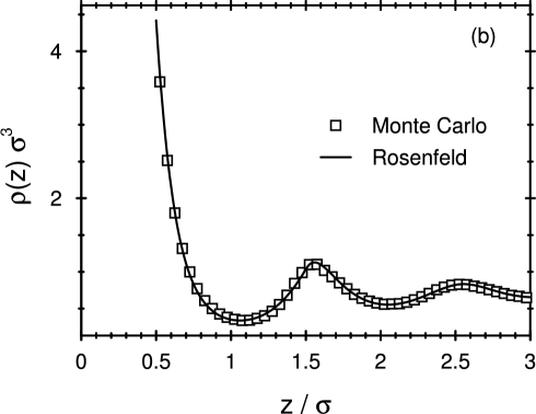
This functional yields excellent results for thermodynamic quantities and for structures in the fluid phase of hard spherical molecules beisbart_roth:depletion . For instance, in Figure 13 the inhomogeneous density profile $\rho(z)$ close to a hard wall is shown as compared to simulation results.
Unfortunately, the functional in Eq. (24) was derived only for hard spheres in three

Figure 13: The density profile of a hard sphere fluid close to a hard wall for a bulk density $\rho(2\sigma)^{3}=0.715$ calculated with the Rosenfeld functional (solid line) as compared to simulation results (squares, Figure from R. Roth, 1999, see beisbart_roth:depletion ). $\sigma$ denotes the diameter of the spheres.

dimensions; however, a proposal has been made for general convex bodies beisbart_rosenfeld:molecular based on an approximative decomposition of $f_{ex}$ in the low density limit. Here, we show how Rosenfeld’s idea of decomposing $f_{ex}$ for spheres beisbart_rosenfeld:free may be extended exactly to non-spherical convex bodies by applying integral geometric techniques such as kinematic formulae and an explicit local expression for the Euler characteristic $\chi(K\cap K^{\prime})$ of two overlapping bodies beisbart_mecke:fundamental . The main idea is to decompose the exact expression for the local excess free energy $f_{ex}[\rho({\mathbf{x}})]$ at low densities in terms of the vector-valued Minkowski functionals. To this end one has to evaluate the configurational integral $\int{\rm d}K=\int{\rm d}R\int{\rm d}{\mathbf{x}}$ over all orientations $R$ and positions ${\mathbf{x}}$ of a body $K=RK_{{\mathbf{x}}}$, namely,

$$\begin{array}[]{cl}&\;\;\;\displaystyle\frac{4\pi}{3}\int{\rm d}{\mathbf{x}}\;\beta f_{ex}[\rho({\mathbf{x}})]\;\;\rightarrow\;\;\frac{2\pi}{3}\int{\rm d}K\int{\rm d}K^{\prime}\;\chi(K_{{\mathbf{x}}}\cap K_{{\mathbf{x}}\,^{\prime}})\;\;\rho({\mathbf{x}})\rho({\mathbf{x}}\,^{\prime})\cr&\cr=&\displaystyle\int_{\mathbb{R}^{d}}{\rm d}{\mathbf{x}}\;\;W_{3}^{0,0}[\rho({\mathbf{x}})]W_{0}^{0,0}[\rho({\mathbf{x}})]\cr\;\;+&\displaystyle\int_{\mathbb{R}^{d}}{\rm d}{\mathbf{x}}\;3W_{1}^{0,0}[\rho({\mathbf{x}})]W_{2}^{0,0}[\rho({\mathbf{x}})]-3W_{1}^{0,1}[\rho({\mathbf{x}})]W_{2}^{0,1}[\rho({\mathbf{x}})]\cr\;\;+&\displaystyle\int_{\mathbb{R}^{d}}{\rm d}{\mathbf{x}}\;\;\int_{{\mathbf{r}}}{\rm d}K_{{\mathbf{x}}}\rho({\mathbf{r}})\int_{{\mathbf{r}}\,^{\prime}}{\rm d}K^{\prime}_{{\mathbf{x}}}\rho({\mathbf{r}}\,^{\prime})\frac{\kappa_{1}-\kappa_{2}}{2}\frac{\left({\mathbf{v}}_{1}{\mathbf{v}}_{1}-{\mathbf{v}}_{2}{\mathbf{v}}_{2}\right)_{ij}({\mathbf{n}}\,^{\prime}{\mathbf{n}}\,^{\prime})_{ij}}{1+{\mathbf{n}}{\mathbf{n}}\,^{\prime}}\cr\end{array}$$ (25)

where ${\mathbf{v}}_{i}$ denotes the principal direction of the curvature $\kappa_{i}$ at ${\mathbf{r}}$ and ${\mathbf{n}}$ (${\mathbf{n}}\,^{\prime}$) are the normal vectors of $RK_{{\mathbf{x}}}$ ($R^{\prime}K_{{\mathbf{x}}}$) at ${\mathbf{r}}$ (${\mathbf{r}}^{\prime}$), respectively. The integral over rotations $R$ and over the surface of the body $K_{{\mathbf{x}}}$ centered at ${\mathbf{x}}$ is written as $\int_{{\mathbf{r}}}{\rm d}K_{{\mathbf{x}}}=\int{\rm d}R\int_{{\mathbf{r}}\in\partial RK_{{\mathbf{x}}}}{\rm d}S^{d-1}$. For spheres with $\kappa_{1}=\kappa_{2}$ one recovers immediately the low-density limit of the intrinsic free energy given by Eq. (24). But unfortunately the last term on the right hand side of Eq. (25) vanishes only for spheres, so that only for hard spheres a finite number of Minkowski functionals is, by accident, sufficient to decompose the excess free energy into contributions stemming alone from the individual bodies, whereas for non-spherical shapes in arbitrary dimensions an infinite number of fundamental curvature measures is required. Nevertheless, based on the most general analytical expression (25), several approximations by a finite number of tensor-valued Minkowski functionals (including the proposal in beisbart_rosenfeld:molecular ) may be proposed and numerically tested which make Rosenfeld’s density functional applicable to general convex bodies, in particular, to spherocylinders and ellipsoids beisbart_mecke:fundamental .

0.7 Conclusions

Concluding, we argue that a new perspective emerges as regards the Minkowski functionals. Instead of marking a small number of distinguished measures (which, of course, they do in a certain sense), the Minkowski functionals are embedded into a more extensive class of Minkowski valuations. These measures generalize the Minkowski functionals without leaving the framework of integral geometry. The essential step to extend the scalar functionals is to replace the motion invariance by motion covariance. This step yields a hierarchy of tensor-valued measures with the Minkowski functionals at the bottom. The higher-rank valuations are moments of the Minkowski functionals where local geometry is weighted with either the position or the normal vector. The full, comprehensive description of the tensor-valued measures is still a mathematical challenge, although some important results concerning the integral geometry of tensor measures have already been achieved, especially in low dimensions (see beisbart_schneider:tensor2 ).
The extensions of the Minkowski functionals are not only mathematically interesting; rather they can be motivated on physical grounds. Since the Minkowski functionals proved to be useful for a number of applications, we are justified to expect that also their generalizations may be suitable tools. Using physical applications at various length scales we exemplified how higher-rank Minkowski valuations complement the information featured by the scalar functionals. From this point of view we hope that the higher-rank Minkowski valuations will become a standard tool for morphometry and some other fields of research concerned with pattern formation.

References

- (1) Abraham, R. G., F. Valdes, H. K. C. Yee, S. van den Bergh (1994): ‘The Morphologies of Distant Galaxies. I. An Automated Classification System’. Ap. J. 432, pp. 75-90.
- (2) Abraham, R. G., S. van den Bergh, K. Glazebrook, R. S. Ellis, B. X. Santiago, P. Surma, R. E. Griffiths (1996): ‘The Morphologies of Distant Galaxies. II. Classifications from the Hubble Space Telescope Medium Deep Survey’. Ap. J. Suppl. 107, pp. 1.
- (3) Alesker, S. (1999): ‘Continuous Rotation Invariant Valuations on Convex Sets’. Ann. of Math. 149 (3), p. 977.
- (4) Alesker, S. (1999): ‘Description of Continuous Isometry Covariant Valuations on Convex Sets’. Geom. Dedicata 74, p. 241.
- (5) Bader, R. F. W. (1990): Atoms in Molecules – A Quantum Theory. (Oxford University Press, Oxford).
- (6) Bartelmann, M., A. Huss, J. M. Colberg, A. Jenkins, F. R. Pearce (1998): ‘Arc Statistics with Realistic Cluster Potentials. IV. Clusters in Different Cosmologies’. Astron. Astrophys. 330, pp. 1-9.
- (7) Beisbart, C. (2001): Measuring Cosmic Structure. Minkowski Valuations and Mark Correlations for Cosmological Morphometry. Ph.D. thesis, Ludwig-Maximilians-Universität München.
- (8) Beisbart, C., T. Buchert, H. Wagner (2001): ‘Morphometry of Spatial Patterns’. Physica A 293/3-4, p. 592.
- (9) Beisbart, C., K. Mecke (2002): ‘Tensor Valuations’. In preparation.
- (10) Beisbart, C., R. Valdarnini, T. Buchert (2001): ‘The Morphological and Dynamical Evolution of Simulated Galaxy Clusters’. Astron. Astrophys. 379, pp. 412–425.
- (11) Block, D. L., I. Puerari, R. J. Buta, R. Abraham, M. Takamiya, A. Stockton (2001): ‘The Duality of Spiral Structure, and a Quantitative Dust Penetrated Morphological Tuning Fork at Low and High Redshift’. In ‘ASP Conf. Ser. 230: Galaxy Disks and Disk Galaxies’.
- (12) Cohen-Tannoudji, C., B. Diu, F. Laloë (1977): Quantum Mechanics: Volume II. (John Wiley & Sons, Chichester), 2nd edition.
- (13) Dahlke, R. (2000), ‘Dynamische Perkolationsmodelle zur Morphologie von Galaxien’, Diploma thesis, Ludwig-Maximilians-Universität München.
- (14) Fischer, P., G. Bernstein, G. Rhee, J. A. Tyson (1997): ‘The Mass Distribution of the Cluster 0957+561 from Gravitational Lensing’. A. J. 113, p. 521.
- (15) Gerola, H., P. E. Seiden (1978): ‘Stochastic Star Formation and Spiral Structure of Galaxies’. Ap. J. 223, pp. 129-135.
- (16) Hadwiger, H. (1957): Vorlesungen über Inhalt, Oberfläche und Isoperimetrie. (Springer Verlag, Berlin).
- (17) Hadwiger, H., C. Meier (1974): ‘Studien zur vektoriellen Integralgeometrie’. Math. Nachr. 56, p. 361.
- (18) Hadwiger, H., R. Schneider (1971): ‘Vektorielle Integralgeometrie’. Elemente der Mathematik 26, p. 49.
- (19) Hubble, E. (1926): ‘Extra-galactic Nebulae’. Ap. J. 64, p. 321.
- (20) Kerscher, M. (2000): ‘Statistical analysis of large-scale structure in the Universe’. In: Statistical Physics and Spatial Statistics: The Art of Analyzing and Modeling Spatial Structures and Pattern Formation, ed. by K. R. Mecke, D. Stoyan, Number 554 in Lecture Notes in Physics (Springer, Berlin), astro-ph/9912329.
- (21) Klain, D. A. (1995): ‘A Short Proof of Hadwiger’s Characterization Theorem’. Mathematika 42, pp. 329-339.
- (22) Kornreich, D. A., M. P. Haynes, R. V. E. Lovelace, L. van Zee (July 2000): ‘Departures From Axisymmetric Morphology and Dynamics in Spiral Galaxies’. A. J. 120, pp. 139-164.
- (23) Lin, C. C., F. H. Shu (1964): ‘On the Spiral structure of Disk Galaxies’. Ap. J. 140, p. 646.
- (24) McMullen, P. (1997): ‘Isometry Covariant Valuations on Convex Bodies’. Rend. Circ. Mat. Palermo (2) 50, pp. 259–271.
- (25) Mecke, K. (2000): ‘Additivity, Convexity, and beyond: Application of Minkowski Functionals in Statistical Physics’. In: Statistical Physics and Spatial Statistics: The Art of Analyzing and Modeling Spatial Structures and Pattern Formation, ed. by K. R. Mecke, D. Stoyan, Number 554 in Lecture Notes in Physics (Springer, Berlin).
- (26) Mecke, K. R. (2002): ‘Fundamental Measure Density Functional for Mixtures of Non-spherical Hard Particles’. In preparation.
- (27) Mohr, J. J., A. E. Evrard, D. E. Fabricant, M. J. Geller (1995): ‘Cosmological Constraints from X-ray Cluster Morphologies’. Ap. J. 447, p. 8.
- (28) Naim, A., O. Lahav, R. J. Buta, H. G. Corwin, G. de Vaucouleurs, A. Dressler, J. P. Huchra, S. van den Bergh, S. Raychaudhury, L. Sodre, M. C. Storrie-Lombardi (1995): ‘A Comparative Study of Morphological Classifications of APM Galaxies’. Mon. Not. R. Astron. Soc. 274, pp. 1107-1125.
- (29) Peacock, J. (1999): Cosmological Physics. (Cambridge University Press, Cambridge).
- (30) Peebles, P. J. E. (1993): Principles of Physical Cosmology. (Princeton University Press, Princeton, New Jersey).
- (31) Reiss, H., H. Frisch, J. L. Lebowitz (1959): ‘Statistical Mechanics of Rigid Spheres’. J. Chem. Phys. 31, pp. 369-380.
- (32) Richstone, D., A. Loeb, E. L. Turner (July 1992): ‘A Lower Limit of the Cosmic Mean Density from the Ages of Clusters of Galaxies’. Ap. J. 393, p. 477.
- (33) Rosenfeld, Y. (1989): ‘Free-energy Model for the Inhomogeneous Hard-sphere Fluid Mixture and Density-functional Theory of Freezing’, Phys. Rev. Lett. 63, pp. 980-983.
- (34) Rosenfeld, Y. (1994): ‘Density Functional Theory of Molecular Fluids: Free-energy Model for the Inhomogeneous Hard-body Fluid’. Phys. Rev. E 50, pp. R3318-3321.
- (35) Roth, R. (1999): Depletion Forces in Hard Sphere Mixtures. Ph.D. thesis, University Wuppertal, (WUB-DIS 99-19).
- (36) Russell, W. S., W. W. Roberts (September 1993): ‘Analysis of the Distribution of Pitch Angles in Model Galactic Disks – Numerical Methods and Algorithms’. Ap. J. 414, pp. 86-97.
- (37) Schmalzing, J., T. Buchert (1997): ‘Beyond Genus Statistics: a Unifying Approach to the Morphology of Cosmic Structure’. Ap. J. Lett. 482, p. L1.
- (38) Schmalzing, J., T. Buchert, A. L. Melott, V. Sahni, B. S. Sathyaprakash, S. F. Shandarin (1999): ‘Disentangling the Cosmic Web. I. Morphology of Isodensity Contours’. Ap. J. 526, p. 568.
- (39) Schneider, P., J. . Ehlers, E. E. Falco (1992): Gravitational Lenses. (Springer-Verlag, Berlin. Also Astronomy and Astrophysics Library).
- (40) Schneider, R. (1972): ‘Krümmungsschwerpunkte konvexer Körper (I)’. Abh. Math. Sem. Univ. Hamburg 37, p. 112.
- (41) Schneider, R. (1972): ‘Krümmungsschwerpunkte konvexer Körper (II)’. Abh. Math. Sem. Univ. Hamburg 37, p. 202.
- (42) Schneider, R. (1993): Convex Bodies: the Brunn-Minkowski Theory. (Cambridge University Press, Cambridge).
- (43) Schneider, R. (2000): ‘Tensor Valuations on Convex Bodies and Integral Geometry’. Rend. Circ. Mat. Palermo, Ser. II, Suppl. 65, p. 295.
- (44) Schneider, R., R. Schuster (2001): ‘Tensor Valuations on Convex Bodies and Integral Geometry, II’. In preparation.
- (45) Seiden, P. E., H. Gerola (1982): ‘Propagating Star Formation and the Structure and Evolution of Galaxies’. Fundamentals of Cosmic Physics 7, pp. 241-4311.
- (46) Serra, J. (ed.) (1994): Mathematical Morphology and its Applications to Image Processing (Kluwer, Dordrecht).