Measuring the Entropy and Testing
the Second Law of Thermodynamics

Abstract

Evidence implies that basic laws of thermodynamics must be tested by experiments. In this paper, an experiment is designed to measure the entropy of a system with at least one known (measurable) equation of state, especially the gas systems. Since the entropy can be measured now, the formulae related to the second law of thermodynamics can be examined by other experiments.

1 Introduction

Among the branches of classical physics, thermodynamics and statistical physics should be the most fantastic ones, which have attracted so many great minds to devote their lives and energy to investigating every topic in these fields. Perhaps among the branches of classical physics, they are the only ones that leave so many open questions, not only in the field of application, but also in their foundations.

In the last century, most of the physcists are attracted to the quantized physics, which can be viewed as the opposite side of classical physics. Although quantization has been the principal melody of physics ever since then, thermodynamics and statistical physics are still vivid with their own open questions. And, even in the so-called modern physics, shadows of thermodynamics and statistical physics are also seen: In the black hole theory, black holes are endowed with the temperature and the entropy[1]. Ideas and concepts of thermodynamics and statistical physics are also applied to the condensed matter theory and the string theory[2]. In fact, the history of quantum theory can be traced back to thermodynamics and statistical physics, where M. Planck use the famous assumption $E=h\nu$ to derive the spectral energy distribution of black bodies, Planck’s formula[3]. What’s more, thermodynamics and statistical physics even paved their way to theories other than physics, such as Shannon’s theory in information theory. Maybe one day someone cheers that they can be used in economics.

On the one hand, thermodynamics and statistical physics are so widely applied. On the other hand, there are so many open questions in them — there are enven no universal theories, neither thermodynamic nor statistical, for non-equilibrium systems. Thus the foundations of thermodynamics, which have been established for more than one hundred years and which are claimed to be valid for arbitrary thermal systems and arbitrary processes, could not be tested by comparing the experimental data with the predictions from a universal thermodynamics. This sounds not so nice to the society of physics.

There are other reasons forcing us to seek for the experimental supports of the basic laws of thermodynamics. They mainly focus on the easily-misunderstood concept, heat, in theromdynamics, which has been widely discussed and quarreled about in literature.

One of such a reason concerns the nature of heat: Is heat a kind of substance accompanying ordinary matter, as it was said in the old-fashioned caloric theory, or just the energy transferred from one body to another as the result of the difference of temperature? As we know, thermodynamics has chosen the latter. But the following consideration will make thermodynamics to sink into trouble.

Recall that the Gibbs free energy $G=\mu n$ for an equilibrium system of pure substance, where $\mu$ is the chemical potential of the substance and $n$ is its amount meassured in moles. Hence the internal energy $U$ of such a system reads

$$U=-pV+TS+\mu n,$$ (1)

or something like that. Now let us consider a subsystem of it which has a virtual boundary that seperates the subsystem from the whole. Now suppose that the virtual boundary of the subsystem expands slowly such that the center of mass remains unchanged and the process can be considered as quasi-static. Since the virtual boundadry and the process are just imaginary, the intensive quantities $p$, $T$ and $\mu$ are constant while the variations of extensive quantities $V$, $S$ and $n$ are proportional, that is,

$$\frac{\Delta V}{V_{0}}=\frac{\Delta S}{S_{0}}=\frac{\Delta n}{n_{0}},$$

where $V_{0}$, $S_{0}$ and $n_{0}$ are the original volume, entropy and amount of the subsystem, respectively. Hence, according to the formulism of thermodynamics, certain amount of heat $Q=T\ \Delta S\neq 0$ must be absorbed by the subsystem after its virtual expansion. In other words, as a virtual surface moves in an equilibrium system, one has to admit that an additional amount of heat, $\;\,\bar{}\mathrm{d}Q=T\,\mathrm{d}S$ has been transferred through it, accompanying the substance that goes through the surface, even though the system is in equilibrium. In this sense, the caloric theory is somehow restored. On the other hand, however, the zeroth law of thermodynamics should have repelled such a possibility, because heat will not be transferred between two systems or two parts of a system provided there is no difference of temperature.

The other reason that we must carefully examine the foundations of thermodynamics comes from the observation of a transformation in the framework of the first law of thermodynamics[4]. Briefly speaking, on the one hand, in order to measure the heat or certain heat-related quantities such as the heat capacity accurately, one must know the internal energy of at least one substance, the water, for example; On the other hand, according to the first law of thermodynamics, the knowledge of the internal energy of water, say, comes from the measurement of heat in various processes of the water. Obviously, such a chick-and-egg problem can not be solved within the framework of the first law of thermodynamics. Hence, from the point of view of the first law of thermodynamics, it is not detectable if the following transformation,

$$U\longrightarrow U^{\prime}=U+\phi,\qquad\;\,\bar{}\mathrm{d}Q\longrightarrow\;\,\bar{}\mathrm{d}Q^{\prime}=\;\,\bar{}\mathrm{d}Q+\mathrm{d}\phi,$$ (2)

is applied to every thermal system, in which $\phi$ is an arbitrary function of thermal variables. However, with the second and the third laws of thermodynamics being considered, the above transformation will be fixed. In other words, in the point of view of the above transformation, a properly chosen internal energy can be assigned to each thermal system such that both the second law and the third law can be satisfied. So one must believe that there are some other methods to measure the heat in an arbitrary quasi-static process, provided that the second law and the third law of thermodynamcs hold for every process.

In this paper, such an experiment is proposed. If the theory of thermodynamics is correct, the entropy of an equilibrium system can be measured. As we have mensioned in the above, however, the motivation of this paper is not to merely give a mothod of how to measuring the entropy, hence the heat in a quasi-static process. The original idea is to test the validity of the whole theory of thermodynamcs, according to which the experimental data possess the features that is described in §4. If otherwise, questions of thermodynamics will arise.

This paper is organized as in the following. In §2, we first labels our ideas of how this experiment is designed. Then follows the outline of the experiment. Based on the same apparatus, there are two kinds of methods of how to measure the entropy of an equilibrium system. In §3, the formulae are derived in deatails. In §4, conclusions and further discussions are given.

2 The Ideas and the Ouline of the Measuring Methods

The ideas of the experiment are described as in the following.

Since, as we have discussed, it remains to be a problem as how to measure the heat, in order to verify the second law, or strictly speaking, the whole set of laws, of thermodynamics, we must design an experiment which avoids measuring quantities related to heat. Hence the heat capacities of various substances will neither be used as the experimental data nor be measured. Instead, only quantities such as the volumes, the pressures, the amounts of concerned substances as well as the temperatures must be measured. This is the basic point of the proposal experiment.

In deriving the formulae, the formulism of thermodynamics is applied. The partial derivatives of the entropy or those of the chemical potentials are replaced of, with the Maxwell’s relations being used whenever possible, because the entropy and the chemical potential cannot be measured directly so far. According to the theory of thermodynamics, all the experimental data should be located on a single line. If one finds this is not the case even after the errors are considered, there must be some questions in the theory of thermodynamics.

In measuring the temperatures, the Kelvin temperature scale is needed in principle. However, in practice this is not so easy to do. This problem is disposed of in the discussion section, §4.

The whole system is assumed to be thermally isolated from its surroundings. This is where most of the errors come from in the measurement. The basic belief must be accepted in the experiment: Systems will not transfer heat if they have the same temperature. We can demand the environment of the system to keep the same temperature as that of the gas in the vessel B (see Figure 1) so that the exchanging heat between the vessel B and the environment can be ignored. Because the method of thermal isolation is a basic skill for measurements in thermodynamics, we believe that this will not be a serious problem.

The experiment is outlined as in the following.

In the experiment, two kinds of gases, denoted respectively by 1 and 2, are put into the vessels A and B, respectively, as shown in Figure 1. The vessel A is totally surrounded by the vessel B so that heat transferred out of the vessel A will be absorbed totally by the gas in the vessel B. The vessel B is thermally isolated from the environment. Techonologically, one may suppose that the environment changes its temperature to keep up with the temperature of the gas in B so that it can be viewed as an adiabatic wall of the the vessel B, because there will be no heat exchanging between the invironment and the vessel B. The pistons, P_A in the vessel A and P_B in the vessel B, can move in and out to change the volumes of the gases. In addition, there is a valve with a pipe inserted into the vessel A, through which small amount of the gas in the vessel A can be bumped in or out of it.

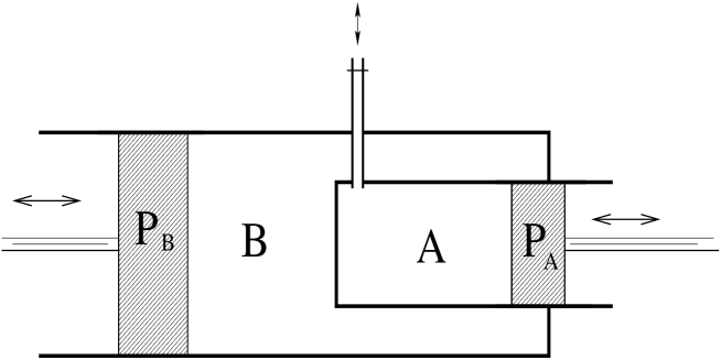
Figure 1: Measuring the entropy of gas systems.

The entropies of two different kinds of gases can be measured at the same time. Let us call the gases 1 and 2, respectively. Suppose that the $i$-th gas is in equilibrium with the volume $V_{i}$, the pressure $p_{i}$, the amount $n_{i}$ in the unit of moles and the chemical potential $\mu_{i}$, where $i=1$ and 2. Separated by the biathermal walls of the vessel $A$, they share the same temperature $T$, which is currently measured in the Kelvin temperature scale.

In the first step, gas 1 and gas 2 are put into the vessel A and B, respectively. the pistons P_A and P_B are adjusted so that the volumes of gas 1 and gas 2 are respectively $V_{1}$ and $V_{2}$. Then, with the pistons fixed, we can always make the gases become thermally equilibrium with each other at the temperature $T$. After that, we make the whole system to be thermally isolated from its surroundings.

Now, a small amount $\mathrm{d}n_{1}$ of gas 1 is bumped into the vessel A through the pipe, with the piston P_A moved slightly meanwhile, making the whole system out of equilibrium. When the thermal equilibrium is established again, we can measure again the common temperature, $T+\mathrm{d}T$, of the gases. Now the volume of gas 1 is $V_{1}+\mathrm{d}V_{1}$, and the amount of gas 1 is $n_{1}+\mathrm{d}n_{1}$.

Then, in the second step, let gas 1 and gas 2 exchange their places, namely, put gas1 and gas 2 into the vessel B and A, respectively. The pistons are adjusted so that the volumes of gas 1 and gas 2 are still $V_{1}$ and $V_{2}$, respectively. Similarly, fixing the pistons, we make the gases absorb or emit certain amount of heat to be in thermal equilibrium with each other at the temperature $T$ as in the first step. After that, the whole system is again thermally isolated from its surroundings.

Now, certain amount of gas 2 is bumped into or out of the vessel A. Meanwhile the piston P_A is adjusted so that the gases are finally in thermal equilibrium with each other at the temperature $T+\mathrm{d}T$. The volume of gas 2 is $V_{2}+\mathrm{d}V_{2}$, and the amount of gas 2 is $n_{2}+\mathrm{d}n_{2}$.

In the above steps, a set of data are measured: $\mathrm{d}V_{1}/\mathrm{d}T$ and $\mathrm{d}n_{1}/\mathrm{d}T$ in the first step, and $\mathrm{d}V_{2}/\mathrm{d}T$ and $\mathrm{d}n_{2}/\mathrm{d}T$ in the second step. Then the following equation

$$\frac{1}{n_{1}}\,\bigg{[}\,V_{1}\,\bigg{(}\frac{\partial p_{1}}{\partial T}\bigg{)}_{V_{1},n_{1}}-S_{1}\,\bigg{]}\,\frac{\mathrm{d}n_{1}}{\mathrm{d}T}-\frac{1}{n_{2}}\,\bigg{[}\,V_{2}\,\bigg{(}\frac{\partial p_{2}}{\partial T}\bigg{)}_{V_{2},n_{2}}-S_{2}\,\bigg{]}\,\frac{\mathrm{d}n_{2}}{\mathrm{d}T}$$ (3)

$$= \bigg{(}\frac{\partial p_{1}}{\partial T}\bigg{)}_{V_{1},n_{1}}\,\frac{\mathrm{d}V_{1}}{\mathrm{d}T}-\bigg{(}\frac{\partial p_{2}}{\partial T}\bigg{)}_{V_{2},n_{2}}\,\frac{\mathrm{d}V_{2}}{\mathrm{d}T}-\frac{\Delta C}{T}$$

should be satisfied, where $S_{1}=S_{1}(T,V_{1},n_{1})$ and $S_{2}=S_{2}(T,V_{2},n_{2})$ are the entropies of gas 1 and gas 2, respectively, and $p_{1}=p_{1}(T,V_{1},n_{1})$ and $p_{2}=p_{2}(T,V_{2},n_{2})$ are respectively the pressures of gas 1 and gas 2, while $\Delta C$ is a constant with the dimension of heat capacity, so small than that of the vessels that it can be ignored, in fact. In the above equation, the partial derivatives of the pressures with respect to the temperature must be measured in other processes.

With several sets of such data, we can fix the entropies of gas 1 and gas 2.

There is another method to measure the entropy of any one of the gases, $S_{1}$, say. Let us put gas 1 into the vessel A and make it to keep equilibrium with the whole system. Suppose the volume, the amount and the temperature of gas 1 are $V_{1}$, $n_{1}$ and $T$, respectively. Again the whole system is thermally isolated from its surroundings. Then we bump some small amount $\mathrm{d}n_{1}$ of gas 1 into the vessel A. At the same time, the piston A is adjusted so that the temperature of gas 1 is kept constant throughout the process. If the volume of gas 1 is now $V_{1}+\mathrm{d}V_{1}$, then the entropy $S_{1}$ of gas 1 at the state $(T,V_{1},n_{1})$ will be

$$S_{1}=\bigg{(}\frac{\partial p_{1}}{\partial T}\bigg{)}_{V_{1},n_{1}}\Big{(}V_{1}-n_{1}\frac{\mathrm{d}V_{1}}{\mathrm{d}n_{1}}\Big{)}.$$ (4)

In the following section, we shall derive the above equation.

3 The Principles of the Experiment

As we know, for a gas system, the first law of thermodynamics can be written in the form of

$$\mathrm{d}U=-p\,\mathrm{d}V+T\,\mathrm{d}S+\mu\,\mathrm{d}n.$$

A Legendre transformation gives the differential of the free energy as

$$\mathrm{d}F=-p\,\mathrm{d}V-S\,\mathrm{d}T+\mu\,\mathrm{d}n,$$ (5)

where the free energy is defined as $F=U-TS.$ Being a homogeneous function of $V$ and $n$ of order 1 for any given temperature $T$, the Euler equation for homogeneous functions of order 1 must be satisfied, in which the temperature is treated as a parameter, giving

$$F=-pV+\mu n.$$ (6)

The option form of the above equation can be $U=-pV+TS+\mu n$ for the internal energy, or[6] $G=\mu n$ for the Gibbs free energy.

One of the most important consequences of the above equations is that the intensive quantities $p$, $T$ and $\mu$ are not functionally independent, namely, their differentials are constrained by an equation

$$\mathrm{d}\mu=\frac{V}{n}\,\mathrm{d}p-\frac{S}{n}\,\mathrm{d}T.$$ (7)

Hence the partial derivative of the chemical potential $\mu$ with respective to the Kelvin temperature $T$ reads

$$\bigg{(}\frac{\partial\mu}{\partial T}\bigg{)}_{V,n}=\frac{V}{n}\bigg{(}\frac{\partial p}{\partial T}\bigg{)}_{V,n}-\frac{S}{n}.$$ (8)

By virtue of the above equation, the heat that is absorbed by an open system in a quasi-static process reads

$$\;\,\bar{}\mathrm{d}Q=T\,\mathrm{d}S=C_{V,n}\,\mathrm{d}T+T\bigg{(}\frac{\partial p}{\partial T}\bigg{)}_{V,n}\mathrm{d}V+\frac{T}{n}\,\bigg{[}S-V\bigg{(}\frac{\partial p}{\partial T}\bigg{)}_{V,n}\bigg{]}\,\mathrm{d}n,$$ (9)

in which the partial derivatives of the entropy $S$ with respect to $V$ and $n$, respectively, have been replaced by the partial derivatives of $p$ and $-\mu$, both with respective to $T$, according to Maxwell’s relations

$$\bigg{(}\frac{\partial S}{\partial V}\bigg{)}_{T,n}=\bigg{(}\frac{\partial p}{\partial T}\bigg{)}_{V,n},\qquad\bigg{(}\frac{\partial S}{\partial n}\bigg{)}_{T,V}=-\bigg{(}\frac{\partial\mu}{\partial T}\bigg{)}_{V,n}.$$ (10)

Now let us focus our attention on the experiment. For the details of experiment, we refer the readers to §2.

In the first step, gas 1 in A with the pressure $p_{1}$ and volume $V_{1}$ is in thermal equilibrium with gas 2 in B with the pressure $p_{2}$ and volume $V_{2}$. The common temperature of them is $T$. When the volume and the amount of gas 1 are slowly changed, the heat absorbed by gas 1 is, according to eq.(9),

$$\;\,\bar{}\mathrm{d}Q_{1}=C_{V,n}^{\ 1}\,\mathrm{d}T+T\bigg{(}\frac{\partial p_{1}}{\partial T}\bigg{)}_{V_{1},n_{1}}\mathrm{d}V_{1}+\frac{T}{n_{1}}\,\bigg{[}S_{1}-V_{1}\bigg{(}\frac{\partial p_{1}}{\partial T}\bigg{)}_{V_{1},n_{1}}\bigg{]}\,\mathrm{d}n_{1},$$

where $C_{V,n}^{\ 1}=C_{V,n}^{\ 1}(T,V_{1},n_{1})$ is the heat capacity of gas 1 at constant volume $V_{1}$ and constant amount $n_{1}$. In this process, since the volume and the amount of gas 2 is remained to be constant, it absorbs some heat

$$\;\,\bar{}\mathrm{d}Q_{2}=C_{V,n}^{\ 2}\,\mathrm{d}T,$$

where $C_{V,n}^{\ 2}=C_{V,n}^{\ 2}(T,V_{2},n_{2})$ is the heat capacity of gas 2 at constant volume $V_{2}$ and constant amount $n_{2}$. Since the whole system is thermally isolated from its surroundings, if the heat absorbed by the vessels and the pistons is assumed to be

$$\;\,\bar{}\mathrm{d}Q_{3}=C\,\mathrm{d}T$$

where $C$ is the effective heat capacity of the vessels and the pistons, there must be the equation

$$\;\,\bar{}\mathrm{d}Q_{1}+\;\,\bar{}\mathrm{d}Q_{2}+\;\,\bar{}\mathrm{d}Q_{3}=0,$$ (11)

namely, the heat emitted by gas 1 will be absorbed by gas 2, the vessels and the pistons, or vice versa. Hence we obtain

$$(C_{V,n}^{\ 1}+C_{V,n}^{\ 2}+C)\,\mathrm{d}T+T\bigg{(}\frac{\partial p_{1}}{\partial T}\bigg{)}_{V_{1},n_{1}}\,\mathrm{d}V_{1}+\frac{T}{n_{1}}\,\bigg{[}S_{1}-V_{1}\bigg{(}\frac{\partial p_{1}}{\partial T}\bigg{)}_{V_{1},n_{1}}\bigg{]}\,\mathrm{d}n_{1}=0.$$

From the above equation, we can see that the whole system, when thermally isolated from its surroundings, has two degrees of freedom. The corresponding variables may be the volume as well as the amount of gas 1 in vessel A. Especially, the temperature of the system can be determined by the above two variables. Thus, for a given state $(T,V_{1},n_{1})$ of gas 1, one may adjust the volume and the amount of it so that the temperature keeps invariant. In such a case, the ratio of the changes of the volume and the amount, $\frac{\mathrm{d}V_{1}}{\mathrm{d}n_{1}}$, will be constrained. On the other hand, if this ratio has been measured, the entropy $S_{1}$ of gas 1 can be determined as that in eq.(4).

Recall that gas 2, the pistons and the vessells won’t absorb any heat provided the temperature remains constant, and that the whole system is thermally isolated. So the above process is not only isothermal, but also adiabatic. On the other hand, according to eq.(9), for an open system, if the process is both isothermal and adiabatic, the entropy of this system can be determined by the equation having the same form as that in the above, only with the subscripts being omitted. However, as discussed in the introduction, it seems that there are some questions in the concept of heat for an open system. This is not the topic of this paper. We will discuss it in other papers.

Technologically, it is very hard to adjust the volume and the amount of gas 1 so that the temperature keeps constant. Ordinarily, the temperature changes in the process, which can be referred to as a parameter of the process, yielding the equation

$$(C_{V,n}^{\ 1}+C_{V,n}^{\ 2}+C)+T\bigg{(}\frac{\partial p_{1}}{\partial T}\bigg{)}_{V_{1},n_{1}}\,\frac{\mathrm{d}V_{1}}{\mathrm{d}T}+\frac{T}{n_{1}}\,\bigg{[}S_{1}-V_{1}\bigg{(}\frac{\partial p_{1}}{\partial T}\bigg{)}_{V_{1},n_{1}}\bigg{]}\,\frac{\mathrm{d}n_{1}}{\mathrm{d}T}=0.$$

Noticing that the heat capacities of gas 1 and gas 2 is totally symmetric in the above equation, one can exchange their sites and repeat the process, obtaining the following equation:

$$(C_{V,n}^{\ 1}+C_{V,n}^{\ 2}+C^{\prime})+T\bigg{(}\frac{\partial p_{2}}{\partial T}\bigg{)}_{V_{2},n_{2}}\,\frac{\mathrm{d}V_{2}}{\mathrm{d}T}+\frac{T}{n_{2}}\,\bigg{[}S_{2}-V_{2}\bigg{(}\frac{\partial p_{2}}{\partial T}\bigg{)}_{V_{2},n_{2}}\bigg{]}\,\frac{\mathrm{d}n_{2}}{\mathrm{d}T}=0.$$

In the above equation, $C^{\prime}$ is the affective heat capacity of the pistons and the vessels when gas 1 is put into the vessel B and 2 into the vessel A.

With the above two equations, we expect the result of the experiment to satisfy eq.(3). In the experiment, we need only to measure the derivatives, with respect to the Kelvin temperature $T$, of the volume and the amount of the gas that is located in the vessel A. The coefficients $(\partial p_{1}/\partial T)_{V_{1}}$ and $(\partial p_{2}/\partial T)_{V_{2}}$ can and must be measured in other processes. In eq.(3), the difference $\Delta C=C^{\prime}-C$ of $C$ and $C^{\prime}$ is so small, compared with either $C$ or $C^{\prime}$, that it can be ignored if the accuracy is not highly needed in the measurement.

In eq.(3), all the quantities except the entropies can be measured in the experiment. If the theory of thermodynamics is correct, the entropies of the gases can be determined from the data. Having the method of measuring the entropy, we can use it to test various statements related to the second law of thermodynamics, such as the law of increase of entropy[8], the Gibbs’ paradox[6]. In addition, if both the entropy and the pressure, as functions of the state of the system, are obtained, the chemical potential can be integrated — at least in principle, according to eq.(7). And one can test whether the Maxwell’s relations such as eqs.(10) is valid for every thermal system, as demanded by the theory of thermodynamics. Especially, the second equation in eqs.(10) can be written as

$$V\,\bigg{(}\frac{\partial p}{\partial T}\bigg{)}_{V,n}=S-n\,\bigg{(}\frac{\partial S}{\partial n}\bigg{)}_{T,V}.$$

It should be verified in the experiments. But, were it verified that $S(T,V,n)$ is a homogeneous function of $V$ and $n$ of order one, the above equation will be equivalent to the first one in eqs.(10).

In the above discussion, the entropy of a thermal system of gas can be measured provided the theory of thermodynamics is correct. As a generalization, we can conclude that, for a thermal system, if one of its equations of state can be determined in experiment, then its entropy can be measured by a properly designed experimental scheme. When its entropy is known, the problem of measuring heat that it absorbs is solved — provided the theory of thermodynamics is correct.

4 Conclusions and Discussions

As we have discussed in the above, the entropy of a pure-gas system, which has three degrees of freedom, can be measured at any given state, $(T,V,n)$, say. For other systems with three degrees of freedom, its entropy can be similarly measured provided one of its equations of state can be measured state by state.

Not that the equation of state is not enough to acquire the knowledge of a thermal system[9]. Even for the simpliest case, an ideal gas, the information of its thermodynamic functions can not be uniquely be determined by the well-known state of equation, $pV=Nk_{B}T$. Apart from the general discussions in the courses, an interesting relativistic case has recently been discussed in [10]. Therefore, the measuring methods for the entropy is really needed even if the equation of state has been known.

Based on the theory of thermodynamics for quasi-static processes, two methods are provided to measure the entropy for a gas system at any given state: One is based on eq.(3), and the other is based on eq.(4).

The first method is not so accurate, because there is an unknown quantity $\Delta C$ which varies from measurement to measurement. Since this is the difference of the effective heat capacities of the vessels as well as the pistons, which are considered to remain constant if the accuracy is not needed to be very high, it is reasonable to be considered as a constant for all the measurements for a given state. And it is even reasonable to drop it out of eq.(3), since it is very small.

The second method is more accurate, but it is more difficult to control. Note that the derivative of $V_{1}$ with respect to $n_{1}$ in eq.(4) is, in fact, the partial derivative $(\partial V_{1}/\partial n_{1})_{T,S_{1}}$. So one can derive that, for the adiabatic isothermal line $V_{1}=V_{1}(T,S_{1},n_{1})$ where $T$ and $S_{1}$ are treated as parameters,

$$\frac{\mathrm{d}^{2}V_{1}}{\mathrm{d}n_{1}^{2}}=-\frac{(\frac{\partial^{2}p_{1}}{\partial T\partial V_{1}})_{n_{1}}}{(\frac{\partial p_{1}}{\partial T})_{V_{1},n_{1}}}\,\bigg{(}\frac{\mathrm{d}V_{1}}{\mathrm{d}n_{1}}-\frac{V_{1}}{n_{1}}\bigg{)}^{2}.$$ (12)

Using this relation, one can make the resulted entropy more accurate.

For the first method, which obeys eq.(3), the data should be located on a 4-dimensional plane spaned by the variables $\mathrm{d}n_{1}/\mathrm{d}T$, $\mathrm{d}n_{2}/\mathrm{d}T$, $\mathrm{d}V_{1}/\mathrm{d}T$ and $\mathrm{d}V_{2}/\mathrm{d}T$. Of course, the partial derivatives, $(\partial p_{1}/\partial T)_{V_{1},n_{1}}$ and $(\partial p_{2}/\partial T)_{V_{2},n_{2}}$, must be measured in other experiments. Although the entropies of two different kinds of gases are measured at the same time, the resulted entropy of one gas should and must have nothing to with the other. All the above features are expected according to the theory of thermodynamics. Were any of them spoiled, questions about the validity of thermodynamics can be asked.

As for the second method, all the measured data of $\mathrm{d}V_{1}/\mathrm{d}n_{1}$ should be consentrated to a definite value, for a given state $(T,V_{1},n_{1})$ of gas 1.

No matter what method is used, the Kelvin temperature scale must be applied in order to obtain the correct value of the entropy/entropies. However, in practice the usual temperature is not the Kelvin temperature. Let the temperature in the experiment be denoted by $\theta$, say. The temperature $T$ being a increasing function of $\theta$, eq.(3) and eq.(4) are turned to be

$$\frac{1}{n_{1}}\,\left[V_{1}\bigg{(}\frac{\partial p_{1}}{\partial\theta}\bigg{)}_{V_{1},n_{1}}-S_{1}\,\frac{\mathrm{d}T}{\mathrm{d}\theta}\ \right]\,\frac{\mathrm{d}n_{1}}{\mathrm{d}\theta}-\frac{1}{n_{2}}\,\left[V_{2}\bigg{(}\frac{\partial p_{2}}{\partial\theta}\bigg{)}_{V_{2},n_{2}}-S_{2}\,\frac{\mathrm{d}T}{\mathrm{d}\theta}\ \right]\,\frac{\mathrm{d}n_{2}}{\mathrm{d}\theta}$$

$$\ \ \ \ \ \ \ \ \ =\bigg{(}\frac{\partial p_{1}}{\partial\theta}\bigg{)}_{V_{1},n_{1}}\frac{\mathrm{d}V_{1}}{\mathrm{d}\theta}-\bigg{(}\frac{\partial p_{2}}{\partial\theta}\bigg{)}_{V_{2},n_{2}}\frac{\mathrm{d}V_{2}}{\mathrm{d}\theta}-\frac{\Delta C}{T}\bigg{(}\frac{\mathrm{d}T}{\mathrm{d}\theta}\bigg{)}^{2},$$ (13)

$$S_{1}\,\frac{\mathrm{d}T}{\mathrm{d}\theta}=\big{(}\frac{\partial p_{1}}{\partial\theta}\bigg{)}_{V_{1},n_{1}}(V_{1}-n_{1}\frac{\mathrm{d}V_{1}}{\mathrm{d}n_{1}}),$$ (14)

respectively. Hence, strictly speaking, we can only measure the quantity

$$\tilde{S}=S\frac{\mathrm{d}T}{\mathrm{d}\theta}$$ (15)

if the derivative of $T$ with respect to $\theta$ is unknown.

It is well known that the errors in thermal experiments are very hard to be evaluated, not only because it is hard to control in the operations, but also because there is hardly methods, in principle, to eliminate the errors. Without quantites related to heat, such as heat capacities, being measured, the accuracy of the measurement methods proposed in this paper is controlable. — At least it is the case in the second method.

As analyzed in the above, the most possible errors come from the following points:

• In what extent we can set the whole system to be thermally isolated from its surroundings;

• In what extent the temperature scale leaves from the Kelvin temperature scale.

And, for the first method, it also depends that the quantity $\Delta C$ varies rather small from measurement to measurement, namely, the effective heat capacity of the vessels and the pistons remains steadily in various processes within the first order of variations of the state.

Now that we have the methods of how to measure the entropy of a system with three degrees of freedom and one equation of state, further experiments can be designed to test the theory of thermodynamics. For example, one can test the law of increasing of entropy, and one can test whether the Maxwell relations such as eqs.(10) hold or not, etc.

Acknowledgments

The author wants to thank Prof. H. Y. Guo and Prof. Z. Zhao for helpful discussions on such topics. He is also thankful to Dr. Xin Wang, Dr. Yu-Guang Wang, and Dr. Lian-You Shan for stimulating discussions. Special appreciations are given to Ji-Jun Li, whose effort on thermodynamics several years ago is a historical backgroud as why the author paid his attention to these topics.

References

- [1] See, for example, J. M. Bardeen, B. Carter and S. W. Hawking, “The Four Laws of Black Hole Mechanics”, Commun. Math. Phys., 31 (1973) 161-170; J. D. Bekenstein, “Black Holes and Entropy”, Phys. Rev., D7 (1973) 2333-2346; J. D. Bekenstein, “Generalized Second Law of Thermodynamics in Black-Hole Physics”, Phys. Rev. D9 (1974) 3292-3300; R. M. Wald, General Relativity, The University of Chicago Press, Chicago 1984.
- [2] There are too many papers in the field of string theory. The following references are not the complete listing concerning thermodynamics of strings: G. Horowitz, “The Origin of Black Hole Entropy in String Theory”, gr-qc/9604051. M. A. Vazquez-Mozo, “Open String Thermodynamics and D-Branes”, Phys. Lett. B388 (1996) 494-503; J. Maldacena, A. Strominger and E. Witten, “Black Hole Entropy in M-Theory”, JHEP 9712 (1997) 002, or hep-th/9711053; M. Cvetic and F. Larsen, “Black Hole Horizons and the Thermodynamics of Strings”, Nucl. Phys. Proc. Suppl. 62 (1998) 443-453; Nucl. Phys. Proc. Suppl. 68 (1998) 55-65; S. A. Abel, J. L. F. Barbon, I. I. Kogan, E. Rabinovici, Some Thermodynamics Aspects of String Theory”, hep-th/99110004; J. P. Peñalba, “Non-paturbative Thermodynamics in Matrix String Theory”, Nucl. Phys. B556 (1999) 152-176; M. Ramon Medrano, N. Sanchez, “Hawking Radiation in String Theory and String Phase of Black Holes”, Phys. Rev. D61 (2000) 084030, hep-th/9906009; A. W. Peet, “TASI lectures on black holes in string theory”, hep-th/0008241; D. Kutasov, D. A. Sahakyan, “Comments on the Thermodynamics of Little String Theory”, JHEP 0102 (2001) 021, or hep-th/0012258;
- [3] See, for example, J. D. Jackson, Classical Electrodynamics, 3rd edition, John Wiley & Sons, Inc., New York 1999, §17-12; or L. D. Landau and E. M. Lifshitz, Statistical Physics, 3rd edition, Part 1 (English Translation by J. B. Sykes and M. J. Kearsley), Pergamon Press, Oxford 1980, §63.
- [4] B. Zhou, “Heat: The Indefinite Concept in Thermodynamics”, unpublished.
- [5] For details and references, see J. D. Jackson, Classical Electrodynamics, 3rd edition, John Wiley & Sons, Inc., New York 1999.
- [6] See, for example, M. W. Zemansky and R. H. Dittman, Heat and Thermodynamics, Sixth edition, McGraw-Hill, 1981.
- [7] L. E. Reichl, A Modern Course in Statistical Physics, §2.4, University of Texas Press, 1980.
- [8] L. D. Landau and E. M. Lifshitz, Statistical Physics, 3rd edition, Part 1 (English Translation by J. B. Sykes and M. J. Kearsley), Pergamon Press, Oxford 1980, §8. [7], §3.3 and §9.2.
- [9] H. B. Callen, Thermodynamics, John Wiley and sons, 1960.
- [10] P. B. Pal, “Thermodynamics of a Classical Ideal Gas at Arbitrary Temperatures”, physics/0201059.