Water wave propagation and scattering over topographical bottoms

Zhen Ye zhen@phy.ncu.edu.tw Department of Physics, National Central University, Chungli, Taiwan 32054
Abstract

Here I present a general formulation of water wave propagation and scattering over topographical bottoms. A simple equation is found and is compared with existing theories. As an application, the theory is extended to the case of water waves in a column with many cylindrical steps.

pacs:
47.10.+g, 47.11.+j, 47.35.+i
††preprint: 0202

I Introduction

There have been many approaches for investigating propagation of water waves over various bottom topographies. A vast body of literature exists. For brevity, I refer the reader to the textbook CCM . Here I would like to derive from the first principle a simple but coherent formulation for the problem. It will be shown that this approximate approach compares favorably with existing approximations when applied to the cases considered previously. The advantage of the present approach is obvious: it is simple, accommodating, systematic, and can be easily numerically programmed. In particular, here I explicitly show that it respectively recovers three previous results for shallow water, deep water, and scattering by rigid cylinders standing in water. I will first give a theory for general bottom topographies. Then I will extend to study the case of water wave propagation and scattering in a column with many cylindrical steps.

II General theory

Consider a water column with an arbitrary bottom topography. We set up the coordinates as follows. Let the $z$ axis be vertical and directed upward. The $x-y$ plane rests at the water surface when it is calm. The depth of the bottom, which describes the bottom topography, is denoted by $h(x,y)$, and the vertical displacement of the water surface is $\eta(x,y,t)$. Now we derive the governing equations for the water waves.

Consider a vertical column with a base differential element $dxdy$ at $(x,y)$. The change rate of the the volume of the column is

$$\frac{\partial}{\partial t}\eta(x,y,t)dxdy.$$

By conservation of mass, this would equal to the net volume flux from all the horizontal directions, i.Β e.

$$\frac{\partial}{\partial t}\eta(x,y,t)dxdy=-\nabla_{\perp}\cdot\left[\int_{-h}^{\eta}dz\vec{v}_{\perp}(x,y,z,t)\right]dxdy,$$

where $\nabla_{\perp}=(\partial_{x},\partial_{y})$, and β€˜βŸ‚perpendicular-to\perp’ denotes the horizontal directions. This gives us the first equation

$$\frac{\partial}{\partial t}\eta(x,y,t)=-\nabla_{\perp}\cdot\left[\int_{-h}^{\eta}dz\vec{v}_{\perp}(x,y,z,t)\right]$$ (1)

The second equation is obtained from the Newton’s second law. From the Euler equation for incompressible ideal flows

$$\partial_{t}\vec{v}+(\vec{v}\cdot\nabla)\vec{v}=-\frac{1}{\rho}\nabla p-\rho g\hat{z},$$

which is valid at $z=0$, with $g$ being the gravity acceleration, and

$$p=\rho g(\eta-z),$$ (2)

we obtain

$$\frac{\partial}{\partial t}\vec{v}_{\perp}(x,y,0,t)+\left[(\vec{v}\cdot\nabla)\vec{v}\right]_{\perp,z=0}=-g\nabla_{\perp}\eta.$$ (3)

Note when the liquid surface tension is included, the following term should be added to Eq.Β (2)

$$\sigma\nabla_{\perp}^{2}\eta,$$ (4)

in which $\sigma$ is the surface tension coefficient. In this paper, for short, we ignore this effect.

Another equation is from the boundary condition at $z=h$, which states

$$\left.\vec{v}\cdot\hat{n}\right|_{z=-h(x,y)}=0,$$ (5)

where $\hat{n}$ is a normal to the bottom. For an incompressible fluid, we also have the following Laplace equation,

$$\nabla\cdot\vec{v}(x,y,z,t)=0,$$ (6)

in the water column.

Equations (1), (3), (5), and (6) are the four fundamental equations for water waves.

II.1 Linearization

For small amplitude waves, i.Β e. $\eta<<h$, we can ignore the non-linear terms in (1) and (3). Such a linearization leads to the following two equations

$$\frac{\partial}{\partial t}\eta(x,y,t)=-\nabla_{\perp}\cdot\left[\int_{-h(x,y)}^{0}dz\vec{v}_{\perp}(x,y,z,t)\right],$$ (7)

and

$$\frac{\partial}{\partial t}\vec{v}_{\perp}(x,y,0,t)+g\nabla_{\perp}\eta(x,y,t)=0.$$ (8)

These two equations together with Eqs.Β (5) and (6) determines scattering of water waves with a bottom topography.

II.2 Propagation approximation

Here we provide an approximate solution to Eqs.Β (7), (8), (5), and (6). The procedure is as follows. When the variation of the bottom topography is smaller than the wavelength (to be determined self-consistently), we can first ignore terms involving $\nabla_{\perp}h$, and solve for the velocity field. For the incompressible fluid, the velocity field can be represented by a scalar field, i.Β e.

$$\vec{v}(x,y,z,t)=\nabla\Phi(x,y,z,t).$$

We write all dynamical variables with a time dependence $e^{-i\omega t}$ (this time fact is dropped afterwards for convenience). This procedure leads to the following equations for $\Phi$.

$$\nabla^{2}\Phi(x,y,z)=0.$$ (9)

with

$$\omega^{2}\Phi(\vec{r},0)+g\frac{\partial}{\partial z}\Phi(\vec{r},0)=0;\ (\vec{r}=(x,y)).$$ (10)

The first approximation is made at the bottom ($z=-h$). The boundary condition at the bottom reads

$$\frac{\partial}{\partial n}\Phi(\vec{r},-h)=\frac{\partial}{\partial z}\Phi(\vec{r},-h)+\nabla_{\perp}\cdot\nabla_{\perp}\Phi(\vec{r},-h)=0.$$ (11)

We approximate that $\hat{n}$ is in the $z$ direction by neglecting the second term in the above equation. This is valid as long as $\nabla_{\perp}h<<kh$. Thus the boundary condition gives

$$\frac{\partial}{\partial z}\Phi(\vec{r},-h)=0.$$ (12)

Note that this condition is exact in the case of step-wise topographical bottoms, to be discussed later. Eqs. (9), (10), and (12) lead to the solution for $\Phi$

$\displaystyle\Phi(x,y,z)$ $\displaystyle=$ $\displaystyle\phi(x,y)\cosh(k(z+h))+$ (13)
$\displaystyle\sum_{n}\phi_{n}(x,y)\cos(k_{n}(z+h)),$

where $k$ satisfies

$$\omega^{2}=gk(x,y)\tanh(k(x,y)h(x,y)),$$ (14)

and $k_{n}$ satisfies

$$\omega^{2}=gk_{n}(x,y)\tan(k_{n}(x,y)h(x,y)).$$ (15)

Here $\phi$ and $\phi_{n}$ are determined by

$$(\nabla^{2}_{\perp}+k^{2})\phi=0,$$ (16)

and

$$(\nabla^{2}_{\perp}-k_{n}^{2})\phi_{n}=0.$$ (17)

Eq.Β (17) leads to evanescent wave solutions.

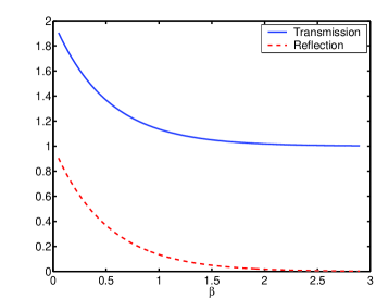
The second approximation is to ignore the summation terms in Eq.Β (13). Such an approximation is based upon the following consideration. The summation terms represent the correction of evanescent waves caused by irregularities such as sudden changes of depth. As these waves are spatially confined, it is reasonable to expect that such a correction will not affect the overall wave propagation, and the general features of the wave propagation. Indeed, when we apply the later approximate solution to the extreme case of propagation of water waves over an infinite step, we find that our results agree reasonably well with that from two other approximate approachesNewman ; Miles . For example, the difference in the reflection results is uniformly less than a few percent for a wide range of frequencies. The largest discrepancy can happen for the transmission results, but the difference is still less than 15%. Furthermore, we find that the derived result is in agreement with that of Kirby for the case of waves over a flat bed with small ripples Kirby . As matter of fact, in this case, it can be shown that after a mathematical manipulationmath Eq.Β (2.11) in Kirby becomes essentially the same as the following Eq.Β (21).

Refer to caption
Figure 1: Transmission and reflection coefficients versus $\beta=kh$ for an infinite step, obtained from Eq.Β (22). While the result for the reflection agrees very well with that in Refs.Β Newman ; Miles , there is some discrepancy in the transmission results within the range of $kh$ between 0.4 to 1.2; the largest discrepancy of about 15% occurs around $kh=0.8$ for the transmission. The legends are adopted from Miles

Under the above approximations, we have

$$\Phi(x,y,z)\approx\phi(x,y)\cosh(k(z+h)),$$ (18)

and

$$v_{\perp}(x,y,z)\approx\cosh(k(z+h))\nabla_{\perp}\phi.$$ (19)

Now taking Eqs.Β (18) and (19) into Eqs.Β (7) and (8), we get

$$\nabla_{\perp}\left(\frac{\tanh(kh)}{k}\nabla_{\perp}\eta\right)+\frac{\omega^{2}}{g}\eta=0.$$ (20)

For convenience, hereafter we write $\nabla_{\perp}$ as $\nabla$ when it acts on the surface wave field $\eta$. That is

$$\nabla\left(\frac{\tanh(kh)}{k}\nabla\eta\right)+\frac{\omega^{2}}{g}\eta=0,$$ (21)

or

$$\nabla\left(\frac{1}{k^{2}}\nabla\eta\right)+\eta=0,$$ (22)

where $k$ satisfies

$$\omega^{2}=gk(\vec{r})\tanh(k(\vec{r})h(\vec{r})).$$ (23)

From this equation, we can have the conditions linking domains with different depths as follows: both $\eta$ and $\frac{\tanh(kh)}{k}\eta=\frac{\omega^{2}}{gk^{2}}\eta$ are continuous across the boundary.

Eq.Β (22) is similar to what is known as the mild-slop approximationCCM :

$$\frac{1}{c}\nabla\left(\frac{c}{k^{2}}\nabla\eta\right)+\eta=0,$$ (24)

where $c$ is given by

$$c=\frac{1}{2}\left(1+\frac{2kh}{\sinh(2kh)}\right).$$ (25)

Eq.Β (24) was derived by a number of authors under the situation that $\nabla h<<kh$. In fact, under this condition it can be shown that Eq.Β (22) and Eq.Β (24) are equivalent.

Note that when the surface tension is added, Eq.Β (21) becomes

$$\nabla\cdot\left[\frac{\tanh(kh)}{k}\nabla\left(\eta-\frac{\sigma}{g\rho}\nabla^{2}\eta\right)\right]+\frac{\omega^{2}}{g}\eta=0,$$ (26)

with Eq.Β (23) becoming

$$\omega^{2}=\left(gk+\frac{\sigma}{\rho}k^{3}\right)\tanh(kh).$$ (27)

II.3 The situation of shallow water or low frequencies

In the case of shallow water, i.Β e. $kh<<1$, we obtain from Eq.Β (21)

$$\nabla\cdot(h\nabla\eta)+\frac{\omega^{2}}{g}\eta=0.$$ (28)

This is the fundamental equation governing the small amplitude waves in shallow water, first derived by LambLamb .

II.4 The situation of deep water or high frequencies

For the deep water case, $hk>>1$, we have

$$k=\frac{\omega^{2}}{g},$$ (29)

and

$$\nabla^{2}\eta+\frac{\omega^{4}}{g^{2}}\eta=0.$$ (30)

In the deep water, the dispersion relation is not affected by the bottom topography.

II.5 Scattering by infinite rigid cylinders

Equations (21) or (22) are also applicable to another class of situation which has been widely studied in the literature. That is, the scattering of water waves by infinite rigid cylinders situated in a uniform water column. When applying (21) or (22) to this case, we find that these two equations are actually exact. In the medium, the wave equation is

$$(\nabla+k^{2})\eta=0$$ (31)

with the boundary condition at the $i$-th cylinder

$$\left.\hat{n}_{i}\cdot\nabla\eta\right|_{i}=0,$$ (32)

obtained as we set the depths of the cylinders equal zero; $\hat{n}_{i}$ is a normal to the interface. In fact, in this case, the problem becomes equivalent to that of acoustic scattering by rigid cylinders, and all the previous acoustic results will followSanchez ; 1998 ; Chen ; Chen1 , such as the interesting phenomenon of deaf bands.

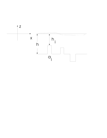
III Water waves in a water column with cylindrical steps

The problem we are now going to consider is illustrated by Fig.Β 2. We consider a water column with a uniform depth $h$. There are $N$ cylindrical steps (or holes when $h_{i}>h$) located in the water. The depths of the steps are measured from the water surface and are denoted by $h_{i}$ and the radii are $a_{i}$. In the realm of the linear wave theory, we study the water wave propagation and scattering by these steps.

Refer to caption
Figure 2: Conceptual layout (side view of the three dimensional coordinates): There are $N$ cylindrical steps located in a water column with depth $h$. The depths of the steps are denoted by $h_{i}(i=1,2,\dots,N)$ measured from the upper surface of the water column, and the radii of the steps are denoted by $a_{i}$. The coordinates are set up as shown. The steps are located at $\vec{r}_{i}$. The $y$-axis lies perpendicularly to the page

III.1 Band structure calculation

When all the steps are with same $h_{1}=h_{2}=\cdots=h_{N}$ and the radius $a$, and are located periodically on the bottom, then we can use Bloch’s theorem to study the water wave propagation. Assume the steps are arranged either in the square or hexagonal lattices, with lattice constant $d$. Here we use the standard plane-wave approachKush ; Msc . By Bloch’s theorem, we can express the field $\eta$ in the following form

$$\eta(x,y)=e^{i\vec{K}\cdot\vec{r}}\sum_{\vec{G}}C(\vec{G},\vec{K})e^{i\vec{G}\cdot\vec{r}},$$ (33)

where $\vec{r}=(x,y)$, $\vec{G}$ is the vector in the reciprocal lattice, and $\vec{K}$ the Bloch vector.

In the present setup, the bottom topograph is periodic, so we have the following expansion

$$\frac{\tanh(kh)}{k}=\sum_{\vec{G}}A(\vec{G})e^{i\vec{G}\cdot\vec{r}},$$ (34)

with

A​(Gβ†’)=(tanh⁑(k1​h1)k1βˆ’tanh⁑(k​h)k)​fs+tanh⁑(k​h)k,𝐴→𝐺subscriptπ‘˜1subscriptβ„Ž1subscriptπ‘˜1π‘˜β„Žπ‘˜subscriptπ‘“π‘ π‘˜β„Žπ‘˜A(\vec{G})=\left(\frac{\tanh(k_{1}h_{1})}{k_{1}}-\frac{\tanh(kh)}{k}\right)f_{s}+\frac{\tanh(kh)}{k}, (35)

for

$$\vec{G}=0;$$

and

$$A(\vec{G})=\left(\frac{\tanh(k_{1}h_{1})}{k_{1}}-\frac{\tanh(kh)}{k}\right)F_{s}(\vec{G}),$$ (36)

for

Gβ†’β‰ 0.→𝐺0\vec{G}\neq 0.

Here $k_{1}$ and $k$ are determined by

$$\omega^{2}=gk_{1}\tanh(k_{1}h_{1})=gk\tanh(kh),$$ (37)

and $f_{s}$ is the filling factor given byMsc

$$f_{s}=\left\{\begin{array}[]{ll}\pi\left(\frac{a}{d}\right)^{2},&\mbox{Square lattice}\\ \frac{2\pi}{\sqrt{3}}\left(\frac{a}{d}\right)^{2},&\mbox{Hexagonal lattice},\end{array}\right.$$

and $F_{s}$ is the structure factor

$$F_{s}(\vec{G})=2f_{s}\frac{J_{1}(|\vec{G}|a)}{|\vec{G}|a}.$$

Substituting Eqs.Β (33) and (34) into Eq.Β (21), we get

$$\sum_{\vec{G}^{\prime}}Q_{\vec{G},\vec{G}^{\prime}}(\vec{K},\omega)C(\vec{G}^{\prime},\vec{K})=0,$$ (38)

with

$$Q_{\vec{G},\vec{G}^{\prime}}(\vec{K},\omega)=[(\vec{G}+\vec{K})\cdot(\vec{G}^{\prime}+\vec{K})]A(\vec{G}-\vec{G}^{\prime})-\frac{\omega^{2}}{g}\delta_{\vec{G},\vec{G}^{\prime}}.$$

The dispersion relation connecting $\vec{K}$ and $\omega$ is determined by the secular equation

$$\mbox{det}\left[(\vec{G}+\vec{K})\cdot(\vec{G}^{\prime}+\vec{K})]A(\vec{G}-\vec{G}^{\prime})-\frac{\omega^{2}}{g}\delta_{\vec{G},\vec{G}^{\prime}}\right]_{\vec{G},\vec{G}^{\prime}}=0.$$ (39)

For the shallow water, we have $\tanh(kh)\approx kh$, and thus $\tanh(kh)/k\approx h$, then by

$$h(x,y)=\sum_{\vec{G}}A(\vec{G})e^{i\vec{G}\cdot\vec{r}},$$ (40)

with

A​(Gβ†’)={(h1βˆ’h)​fs+h,for​Gβ†’=0;(h1βˆ’h)​Fs​(Gβ†’),for​Gβ†’β‰ 0.𝐴→𝐺casessubscriptβ„Ž1β„Žsubscriptπ‘“π‘ β„Žfor→𝐺0subscriptβ„Ž1β„Žsubscript𝐹𝑠→𝐺for→𝐺0A(\vec{G})=\left\{\begin{array}[]{ll}(h_{1}-h)f_{s}+h,&\mbox{for}\ \vec{G}=0;\\ (h_{1}-h)F_{s}(\vec{G}),&\mbox{for}\ \vec{G}\neq 0.\end{array}\right. (41)

III.2 Multiple scattering theory

The shallow water wave propagation in the water column with cylindrical steps can also be investigated by the multiple scattering theory. Without requiring that all the steps are the same, we can develop a general formulism.

In the water column, the wave equation reads

$$(\nabla^{2}+k^{2})\eta=0,$$ (42)

with $k$ being given by

$$\omega^{2}=gk\tanh(kh)$$

Within the range of the $i$-th step, the wave equation is

$$(\nabla^{2}+k_{i}^{2})\eta_{i}=0,$$ (43)

with

$$\omega^{2}=gk\tanh(kh)$$

At the boundary of the step, the boundary conditions are

$$\left.\frac{\tanh(k_{i}h_{i})}{k_{i}}\hat{n}\cdot\nabla\eta_{i}\right|_{\partial\Omega_{i}}=\left.\frac{\tanh(k_{i}h_{i})}{k_{i}}\hat{n}\cdot\nabla\eta\right|_{\partial\Omega_{i}},$$ (44)

derived from the conservation of mass, and

$$\left.\eta_{i}\right|_{\partial\Omega_{i}}=\left.\eta\right|_{\partial\Omega_{i}}.$$ (45)

Here $\partial\Omega_{i}$ denotes the boundary, and $\hat{n}$ is the outward normal at the boundary.

Equations (42) and (43) with the boundary conditions in (44) and (45) completely determine the shallow water wave scattering by an ensemble of cylindrical steps located vertically in the uniform water column. By inspecting, we see that this set of equations is essentially the same as the two dimensional acoustic scattering by an array of parallel cylindersTwersky ; Chen . We following Chen to study the scattering of shallow water waves in the present system.

Consider a line source located at rβ†’ssubscriptβ†’π‘Ÿπ‘ \vec{r}_{s}. Without the cylinder steps, the wave is governed by

(βˆ‡2+k2)​G​(rβ†’βˆ’rβ†’s)=βˆ’4​π​δ(2)​(rβ†’βˆ’rβ†’s),superscriptβˆ‡2superscriptπ‘˜2πΊβ†’π‘Ÿsubscriptβ†’π‘Ÿπ‘ 4πœ‹superscript𝛿2β†’π‘Ÿsubscriptβ†’π‘Ÿπ‘ (\nabla^{2}+k^{2})G(\vec{r}-\vec{r}_{s})=-4\pi\delta^{(2)}(\vec{r}-\vec{r}_{s}), (46)

where $H_{0}^{(1)}$ is the zero-th order Hankel function of the first kind. In the cylindrical coordinates, the solution is

G​(rβ†’βˆ’rβ†’s)=i​π​H0(1)​(k​|rβ†’βˆ’rβ†’s|).πΊβ†’π‘Ÿsubscriptβ†’π‘Ÿπ‘ iπœ‹superscriptsubscript𝐻01π‘˜β†’π‘Ÿsubscriptβ†’π‘Ÿπ‘ G(\vec{r}-\vec{r}_{s})=\mbox{i}\pi H_{0}^{(1)}(k|\vec{r}-\vec{r}_{s}|). (47)

In this section, β€˜i’ stands for $\sqrt{-1}$.

With $N$ cylinder steps located at $\vec{r}_{i}$ ($i=1,2,\cdots,N$), the scattered wave from the $j$-th step can be written as

Ξ·s​(rβ†’,rβ†’j)=βˆ‘n=βˆ’βˆžβˆži​π​Anj​Hn(1)​(k​|rβ†’βˆ’rβ†’j|)​ei​n​ϕrβ†’βˆ’rβ†’j,subscriptπœ‚π‘ β†’π‘Ÿsubscriptβ†’π‘Ÿπ‘—superscriptsubscript𝑛iπœ‹superscriptsubscript𝐴𝑛𝑗superscriptsubscript𝐻𝑛1π‘˜β†’π‘Ÿsubscriptβ†’π‘Ÿπ‘—superscript𝑒i𝑛subscriptitalic-Ο•β†’π‘Ÿsubscriptβ†’π‘Ÿπ‘—\eta_{s}(\vec{r},\vec{r}_{j})=\sum_{n=-\infty}^{\infty}\mbox{i}\pi A_{n}^{j}H_{n}^{(1)}(k|\vec{r}-\vec{r}_{j}|)e^{\mbox{i}n\phi_{\vec{r}-\vec{r}_{j}}}, (48)

where $H_{n}^{(1)}$ is the $n$-th order Hankel function of the first kind. $A_{n}^{i}$ is the coefficient to be determined, and $\phi_{\vec{r}-\vec{r}_{j}}$ is the azimuthal angle of the vector $\vec{r}-\vec{r}_{i}$ relative to the positive $x$-axis.

The total wave incident around the $i$-th scatterer $\eta_{in}^{i}(\vec{r})$ is a superposition of the direct contribution from the source Ξ·0​(rβ†’)=G​(rβ†’βˆ’rβ†’s)subscriptπœ‚0β†’π‘ŸπΊβ†’π‘Ÿsubscriptβ†’π‘Ÿπ‘ \eta_{0}(\vec{r})=G(\vec{r}-\vec{r}_{s}) and the scattered waves from all other scatterers:

Ξ·i​ni​(rβ†’)=Ξ·0​(rβ†’)+βˆ‘j=1,jβ‰ iNΞ·s​(rβ†’,rβ†’j).superscriptsubscriptπœ‚π‘–π‘›π‘–β†’π‘Ÿsubscriptπœ‚0β†’π‘Ÿsuperscriptsubscriptformulae-sequence𝑗1𝑗𝑖𝑁subscriptπœ‚π‘ β†’π‘Ÿsubscriptβ†’π‘Ÿπ‘—\eta_{in}^{i}(\vec{r})=\eta_{0}(\vec{r})+\sum_{j=1,j\neq i}^{N}\eta_{s}(\vec{r},\vec{r}_{j}). (49)

In order to separate the governing equations into modes, we can express the total incident wave in term of the modes about $\vec{r_{i}}$:

$$\eta_{in}^{i}(\vec{r})=\sum_{n=-\infty}^{\infty}B_{n}^{i}J_{n}(k|\vec{r}-\vec{r_{i}}|)e^{\mbox{i}n\phi_{\vec{r}-\vec{r_{i}}}}.$$ (50)

The expansion is in terms of Bessel functions of the first kind $J_{n}$ to ensure that $\eta_{in}^{i}(\vec{r})$ does not diverge as $\vec{r}\rightarrow\vec{r_{i}}$. The coefficients $B_{n}^{i}$ are related to the $A_{n}^{j}$ in equation (48) through equation (49). A particular $B_{n}^{i}$ represents the strength of the $n$-th mode of the total incident wave on the $i$-th scatterer with respect to the $i$-th scatterer’s coordinate system (i.e. around $\vec{r_{i}}$). In order to isolate this mode on the right hand side of equation (49), and thus determine a particular $B_{n}^{i}$ in terms of the set of $A_{n}^{j}$, we need to express Ξ·s​(rβ†’,rjβ†’)subscriptπœ‚π‘ β†’π‘Ÿβ†’subscriptπ‘Ÿπ‘—\eta_{s}(\vec{r},\vec{r_{j}}), for each jβ‰ i𝑗𝑖j\neq i, in terms of the modes with respect to the $i$-th scatterer. In other words, we want Ξ·s​(rβ†’,rjβ†’)subscriptπœ‚π‘ β†’π‘Ÿβ†’subscriptπ‘Ÿπ‘—\eta_{s}(\vec{r},\vec{r_{j}}) in the form

Ξ·s​(rβ†’,rjβ†’)=βˆ‘n=βˆ’βˆžβˆžCnj,i​Jn​(k​|rβ†’βˆ’riβ†’|)​ei​ϕrβ†’βˆ’riβ†’.subscriptπœ‚π‘ β†’π‘Ÿβ†’subscriptπ‘Ÿπ‘—superscriptsubscript𝑛superscriptsubscript𝐢𝑛𝑗𝑖subscriptπ½π‘›π‘˜β†’π‘Ÿβ†’subscriptπ‘Ÿπ‘–superscript𝑒isubscriptitalic-Ο•β†’π‘Ÿβ†’subscriptπ‘Ÿπ‘–\eta_{s}(\vec{r},\vec{r_{j}})=\sum_{n=-\infty}^{\infty}C_{n}^{j,i}J_{n}(k|\vec{r}-\vec{r_{i}}|)e^{\mbox{i}\phi_{\vec{r}-\vec{r_{i}}}}. (51)

This can be achieved (i.e. $C_{n}^{j,i}$ expressed in terms of $A_{n}^{i}$) through the following addition theoremaddition :

$\displaystyle H_{n}^{(1)}(k|\vec{r}-\vec{r_{j}}|)e^{\mbox{i}n\phi_{\vec{r}-\vec{r_{j}}}}=e^{\mbox{i}n\phi_{\vec{r_{i}}-\vec{r_{j}}}}\times$
$\displaystyle\sum_{l=-\infty}^{\infty}H_{n-l}^{(1)}(k|\vec{r_{i}}-\vec{r_{j}}|)e^{-\mbox{i}l\phi_{\vec{r_{i}}-\vec{r_{j}}}}J_{l}(k|\vec{r}-\vec{r_{i}}|)e^{\mbox{i}l\phi_{\vec{r}-\vec{r_{i}}}}.$ (52)

Taking equation (III.2) into equation (48), we have

Ξ·s​(rβ†’,rjβ†’)=βˆ‘n=βˆ’βˆžβˆži​π​Anj​ei​n​ϕriβ†’βˆ’rjβ†’subscriptπœ‚π‘ β†’π‘Ÿβ†’subscriptπ‘Ÿπ‘—superscriptsubscript𝑛iπœ‹superscriptsubscript𝐴𝑛𝑗superscript𝑒i𝑛subscriptitalic-Ο•β†’subscriptπ‘Ÿπ‘–β†’subscriptπ‘Ÿπ‘—\displaystyle\eta_{s}(\vec{r},\vec{r_{j}})=\sum_{n=-\infty}^{\infty}\mbox{i}\pi A_{n}^{j}e^{\mbox{i}n\phi_{\vec{r_{i}}-\vec{r_{j}}}}
$\displaystyle\sum_{l=-\infty}^{\infty}H_{n-l}^{(1)}(k|\vec{r_{i}}-\vec{r_{j}}|)e^{-\mbox{i}l\phi_{\vec{r_{i}}-\vec{r_{j}}}}J_{l}(k|\vec{r}-\vec{r_{i}}|)e^{\mbox{i}l\phi_{\vec{r}-\vec{r_{i}}}}.$ (53)

Comparing with equation (51), we see that

$$C_{n}^{j,i}=\sum_{l=-\infty}^{\infty}\mbox{i}\pi A_{l}^{j}H_{l-n}^{(1)}(k|\vec{r_{i}}-\vec{r_{j}}|)e^{\mbox{i}(l-n)\phi_{\vec{r_{i}}-\vec{r_{j}}}}$$ (54)

Now we can relate $B_{n}^{i}$ to $C_{n}^{j,i}$ (and thus to $A_{l}^{j}$) through equation (49). First note that through the addition theorem the source wave can be written,

Ξ·0​(rβ†’)=i​π​H0(1)​(k​|rβ†’βˆ’rβ†’s|)=βˆ‘l=βˆ’βˆžβˆžSli​Jl​(k​|rβ†’βˆ’riβ†’|)​ei​l​ϕrβ†’βˆ’riβ†’,subscriptπœ‚0β†’π‘Ÿiπœ‹superscriptsubscript𝐻01π‘˜β†’π‘Ÿsubscriptβ†’π‘Ÿπ‘ missing-subexpressionsuperscriptsubscript𝑙superscriptsubscript𝑆𝑙𝑖subscriptπ½π‘™π‘˜β†’π‘Ÿβ†’subscriptπ‘Ÿπ‘–superscript𝑒i𝑙subscriptitalic-Ο•β†’π‘Ÿβ†’subscriptπ‘Ÿπ‘–\begin{array}[]{lll}\eta_{0}(\vec{r})&=&\mbox{i}\pi H_{0}^{(1)}(k|\vec{r}-\vec{r}_{s}|)\\ &=&\sum_{l=-\infty}^{\infty}S_{l}^{i}J_{l}(k|\vec{r}-\vec{r_{i}}|)e^{\mbox{i}l\phi_{\vec{r}-\vec{r_{i}}}},\end{array} (55)

where

Sli=i​π​Hβˆ’l(1)​(k​|riβ†’βˆ’rβ†’s|)​eβˆ’i​l​ϕriβ†’.superscriptsubscript𝑆𝑙𝑖iπœ‹superscriptsubscript𝐻𝑙1π‘˜β†’subscriptπ‘Ÿπ‘–subscriptβ†’π‘Ÿπ‘ superscript𝑒i𝑙subscriptitalic-Ο•β†’subscriptπ‘Ÿπ‘–S_{l}^{i}=\mbox{i}\pi H_{-l}^{(1)}(k|\vec{r_{i}}-\vec{r}_{s}|)e^{-\mbox{i}l\phi_{\vec{r_{i}}}}. (56)

Matching coefficients in equation (49) and using equations (50), (51) and (55), we have

Bni=Sni+βˆ‘j=1,jβ‰ iNCnj,i,superscriptsubscript𝐡𝑛𝑖superscriptsubscript𝑆𝑛𝑖superscriptsubscriptformulae-sequence𝑗1𝑗𝑖𝑁superscriptsubscript𝐢𝑛𝑗𝑖B_{n}^{i}=S_{n}^{i}+\sum_{j=1,j\neq i}^{N}C_{n}^{j,i}, (57)

or, expanding $C_{n}^{j,i}$,

Bni=Sni+βˆ‘j=1,jβ‰ iNβˆ‘l=βˆ’βˆžβˆži​π​Alj​Hlβˆ’n(1)​(k​|riβ†’βˆ’rjβ†’|)​ei​(lβˆ’n)​ϕriβ†’βˆ’rjβ†’.superscriptsubscript𝐡𝑛𝑖superscriptsubscript𝑆𝑛𝑖superscriptsubscriptformulae-sequence𝑗1𝑗𝑖𝑁superscriptsubscript𝑙iπœ‹superscriptsubscript𝐴𝑙𝑗superscriptsubscript𝐻𝑙𝑛1π‘˜β†’subscriptπ‘Ÿπ‘–β†’subscriptπ‘Ÿπ‘—superscript𝑒i𝑙𝑛subscriptitalic-Ο•β†’subscriptπ‘Ÿπ‘–β†’subscriptπ‘Ÿπ‘—B_{n}^{i}=S_{n}^{i}+\sum_{j=1,j\neq i}^{N}\sum_{l=-\infty}^{\infty}\mbox{i}\pi A_{l}^{j}H_{l-n}^{(1)}(k|\vec{r_{i}}-\vec{r_{j}}|)e^{\mbox{i}(l-n)\phi_{\vec{r_{i}}-\vec{r_{j}}}}. (58)

At this stage, both the $S_{n}^{i}$ are known, but both $B_{n}^{i}$ and $A_{l}^{j}$ are unknown. Boundary conditions will give another equation relating them.

The wave inside the $i$-th scatterer can be expressed as

$$\eta_{int}^{i}(\vec{r})=\sum_{n=-\infty}^{\infty}D_{n}^{i}J_{n}(k_{i}|\vec{r}-\vec{r_{i}}|)e^{\mbox{i}n\phi_{\vec{r}-\vec{r_{i}}}}.$$ (59)

Taking Eqs.Β (48), (50), and (59) into the boundary conditions in (44) and (45), we have

$\displaystyle B_{n}^{i}J_{n}(ka_{i})+\mbox{i}\pi A_{n}^{i}H_{n}^{(1)}(ka_{i})$ $\displaystyle=$ $\displaystyle D_{n}^{i}J_{n}(k_{i}a_{i})$ (60)
$\displaystyle B_{n}^{i}J_{n}^{\prime}(ka_{i})+\mbox{i}\pi A_{n}^{i}H_{n}^{(1)\prime}(ka_{i})$ $\displaystyle=$ $\displaystyle\frac{\tanh(h_{i}k_{i})}{\tanh(hk)}D_{n}^{i}J_{n}^{\prime}(k_{i}a_{i}),$

where β€˜β€²β€™ refers to the derivative. Elimination of $D_{n}^{i}$ gives

$$B_{n}^{i}=\mbox{i}\pi\Gamma_{n}^{i}A_{n}^{i},$$ (62)

where

$$\Gamma_{n}^{i}=\frac{H_{n}^{(1)}(ka_{i})J_{n}^{\prime}(k_{i}a_{i})-\frac{\tanh(kh)}{\tanh(k_{i}h_{i})}H_{n}^{(1)\prime}(ka_{i})J_{n}(k_{i}a_{i})}{\frac{\tanh(kh)}{\tanh(k_{i}h_{i})}J_{n}^{\prime}(ka_{i})J_{n}(k_{i}a_{i})-J_{n}(ka_{i})J_{n}^{\prime}(k_{i}a_{i})}.$$ (63)

If we define

Tni=Sni/i​π=Hβˆ’n(1)​(k​|riβ†’βˆ’rβ†’s|)​eβˆ’i​n​ϕriβ†’superscriptsubscript𝑇𝑛𝑖superscriptsubscript𝑆𝑛𝑖iπœ‹superscriptsubscript𝐻𝑛1π‘˜β†’subscriptπ‘Ÿπ‘–subscriptβ†’π‘Ÿπ‘ superscript𝑒i𝑛subscriptitalic-Ο•β†’subscriptπ‘Ÿπ‘–T_{n}^{i}=S_{n}^{i}/\mbox{i}\pi=H_{-n}^{(1)}(k|\vec{r_{i}}-\vec{r}_{s}|)e^{-\mbox{i}n\phi_{\vec{r_{i}}}} (64)

and

Gl,ni,j=Hlβˆ’n(1)​(k​|riβ†’βˆ’rjβ†’|)​ei​(lβˆ’n)​ϕriβ†’βˆ’rjβ†’,iβ‰ jformulae-sequencesuperscriptsubscript𝐺𝑙𝑛𝑖𝑗superscriptsubscript𝐻𝑙𝑛1π‘˜β†’subscriptπ‘Ÿπ‘–β†’subscriptπ‘Ÿπ‘—superscript𝑒i𝑙𝑛subscriptitalic-Ο•β†’subscriptπ‘Ÿπ‘–β†’subscriptπ‘Ÿπ‘—π‘–π‘—G_{l,n}^{i,j}=H_{l-n}^{(1)}(k|\vec{r_{i}}-\vec{r_{j}}|)e^{\mbox{i}(l-n)\phi_{\vec{r_{i}}-\vec{r_{j}}}},i\neq j (65)

then equation (58) becomes

Ξ“ni​Aniβˆ’βˆ‘j=1,jβ‰ iNβˆ‘l=βˆ’βˆžβˆžGl,ni,j​Alj=Tni.superscriptsubscriptΓ𝑛𝑖superscriptsubscript𝐴𝑛𝑖superscriptsubscriptformulae-sequence𝑗1𝑗𝑖𝑁superscriptsubscript𝑙superscriptsubscript𝐺𝑙𝑛𝑖𝑗superscriptsubscript𝐴𝑙𝑗superscriptsubscript𝑇𝑛𝑖\Gamma_{n}^{i}A_{n}^{i}-\sum_{j=1,j\neq i}^{N}\sum_{l=-\infty}^{\infty}G_{l,n}^{i,j}A_{l}^{j}=T_{n}^{i}. (66)

If the value of $n$ is limited to some finite range, then this is a matrix equation for the coefficients $A_{n}^{i}$. Once solved, the total wave at any point outside all cylinder steps is

$\displaystyle\eta(\vec{r})$ $\displaystyle=$ i​π​H0(1)​(k​|rβ†’βˆ’rβ†’s|)+limit-fromiπœ‹superscriptsubscript𝐻01π‘˜β†’π‘Ÿsubscriptβ†’π‘Ÿπ‘ \displaystyle\mbox{i}\pi H_{0}^{(1)}(k|\vec{r}-\vec{r}_{s}|)+ (67)
$\displaystyle\sum_{i=1}^{N}\sum_{n=-\infty}^{\infty}\mbox{i}\pi A_{n}^{i}H_{n}^{(1)}(k|\vec{r}-\vec{r_{i}}|)e^{\mbox{i}n\phi_{\vec{r}-\vec{r_{i}}}}.$

We must stress that total wave expressed by eq.Β (67) incorporate all orders of multiple scattering. We also emphasize that the above derivation is valid for any configuration of the cylinder steps. In other words, eq.Β (67) works for situations that the steps can be placed either randomly or orderly.

For the special case of shallow water ($kh<<1$), we need just replace $\Gamma_{n}^{i}$ in Eq.Β (63) by

$$\Gamma_{n}^{i}=\frac{H_{n}^{(1)}(ka_{i})J_{n}^{\prime}(k_{i}a_{i})-\sqrt{\frac{h}{h_{i}}}H_{n}^{(1)\prime}(ka_{i})J_{n}(k_{i}a_{i})}{\sqrt{\frac{h}{h_{i}}}J_{n}^{\prime}(ka_{i})J_{n}(k_{i}a_{i})-J_{n}(ka_{i})J_{n}^{\prime}(k_{i}a_{i})}.$$ (68)

IV Summary

In summary, here we have presented a general theory for studying gravity waves over bottom topographies. The results have been extended to the case of step-wise bottom structures. The model presented here is simple and may facilitate the research on many unusual wave phenomena such as wave localizationIm ; Emile .

Acknowledgments

Discussion with H.-P. Fang and X.-H. Hu at Fudan University are appreciated. The comments from X.-H. Hu are acknowledged. The helps from K.-H. Wang, B.Β Gupta, and P.-C. (Betsy) Cheng are also thanked.

References

  • (1) C.-C. Mei, The Applied Dynamics of Ocean Surface Waves, (World Scientific, Singapore, 1989).
  • (2) J. N. Newman, J. Fluid Mech. 23, 399 (1965).
  • (3) J. W. Miles, J. Fluid Mech. 28, 755 (1967).
  • (4) Use the identity $\nabla_{\perp}k=\frac{-\omega^{2}\nabla_{\perp}h}{cc_{g}\sinh(2kh)}.$
  • (5) J. T. Kirby, J. Fluid Mech. 162, 171 (1986).
  • (6) H. Lamb, Hydrodynamics, (Cambridge, New York, 1932)
  • (7) J. V. SΓ‘nchez-PΓ©rez, et al., Phys. Rev. Lett. 80, 5325 (1998).
  • (8) W. M. Robertson and J. F. Rudy III, J. Acoust. Soc. Am. 104, 694 (1998).
  • (9) Y. Y. Chen and Z. Ye, Phys. Rev. E 64, 036616 (2001).
  • (10) Y. Y. Chen and Z. Ye, Phys. Rev. Lett. 87, 184301 (2001)
  • (11) M. S. Kushwaha, Int. J. Mod. Phys. B10, 977 (1996).
  • (12) Y.-Y. Chen, M. Sc. thesis, National Central University, http://thesis.lib.ncu.edu.tw (2001).
  • (13) V. Twersky, J. Acoust. Soc. Am. 24, 42 (1951).
  • (14) I. S Gradshteyn, I. M. Ryzhik, and A. Jeffrey, Table of Integrals, Series, and Products, 5th Ed., (Academic Press, New York, 1994).
  • (15) P. W. Anderson, Phys. Rev. 109, 1492 (1958).
  • (16) E. Hoskinson and Z. Ye, Phys. Rev. Lett. 83, 2734 (1999).