From Laser Induced Line Narrowing To Electromagnetically Induced Transparency:
Closed System Analysis

Abstract. Laser induced line narrowing effect, discovered more than thirty years ago, can also be applied to recent studies in high resolution spectroscopy based on electromagnetically induced transparency. In this paper we first present a general form of the transmission width of electromagnetically induced transparency in a homogeneously broadened medium. We then analyze a Doppler broadened medium by using a Lorentzian function as the atomic velocity distribution. The dependence of the transmission linewidth on the driving field intensity is discussed and compared to the laser induced line narrowing effect. This dependence can be characterized by a parameter which can be regarded as “the degree of optical pumping”.

PACS: 32.70.Jz, 42.50.Gy, 42.55.-f, 42.65.-k

Over the last decade, considerable attention has been paid to the studies of the atomic coherence effects and their applications [1, 2]. The technique of Electromagnetically Induced Transparency (EIT) which makes an opaque medium become transparent by applying an external coherent radiation field [3, 4], yields various applications from enhancement of nonlinear optical processes [5, 6, 7], to slow light [8, 9, 10, 11, 12, 13, 14]. In addition to the elimination of absorption, the absorption profile reveals a narrow transmission line, which has been applied to high resolution spectroscopy and high sensitivity magnetometer [15, 16, 17, 18].

Since many of these experiments are performed in an atomic cell configuration, the Doppler broadening effect on EIT is an important concern. Recent theoretical investigations of Doppler broadening effects on EIT, however, has been focused mainly on the existence of EIT for certain configurations [19, 20, 21]. The issue of EIT linewidth for a Doppler broadened medium has been lately addressed by Taichenachev and coworkers [22]. As the width of transmission line is directly related to the dispersion near the EIT resonance, it is also a key issue in dispersive measurements.

In a three-level $\Lambda$-type system if the system is homogeneously broadened, as is well known, EIT can be achieved when the intensity of the driving field ($\Omega^{2}$) is larger than the product of the decay rate of the coherence between the lower levels ($\gamma_{bc}$) and the homogeneous linewidth ($\gamma$). Then, if the system is inhomogeneously broadened (say, with the width $W_{D}$), one might guess that EIT can be achieved when $\Omega^{2}$ is larger than $\gamma_{bc}W_{D}$ instead of $\gamma_{bc}\gamma$. This is not so. We show that one can still have EIT when $\Omega^{2}\gg{\gamma_{bc}\gamma}$ even in the case of inhomogeneous broadening.

For the spectral width of EIT, if the system is homogeneously broadened, the two absorption lines are separated approximately by the Rabi frequency of the driving field $\Omega$ when $\Omega$ is larger than the homogeneous linewidth $\gamma$. When $\Omega\ll\gamma$, it becomes $\Omega^{2}/\gamma$. Then, if the system is inhomogeneously broadened, it might be inferred that the EIT width goes as $\Omega$ when $\Omega$ is larger than the inhomogeneous linewidth $W_{D}$, and becomes $\Omega^{2}/W_{D}$ as $\Omega\ll W_{D}$.

In the literature, however, we find that the narrow feature superimposed on the Doppler broadened profile has been studied more than thirty years ago. Laser induced line narrowing effect was discovered by Feld and Javan [23] and the spectral width of the narrow line was shown to be linearly proportional to the driving field Rabi frequency. Various aspects of this effect has been investigated by Hänsch and Toschek [24], and it was also called nonlinear interference effects [25]. In a recent article [26], it has been proposed that this laser induced line narrowing can be applied to the recent experiments based on EIT and the spectral line of the EIT resonance can be narrower in a Doppler broadened system than in a homogeneously broadened system. Here we analyze these ideas in detail and demonstrate the power broadening of the linewidth of EIT resonance in a Doppler broadened system.

Under the condition of $\Omega\ll W_{D}$, there are again two different regimes of EIT width: In one limit it is proportional to the Rabi frequency of the driving field, which has the same expression as the spectral width shown in the study of laser induced line narrowing [23]. As the driving field gets strong, it becomes power broadened and indeed has a form proportional to the intensity of driving field (as $\Omega^{2}/W_{D}$).

This paper is organized as follows: In Sec. I we set up our model scheme of the three-level system and the transmission width of EIT in a homogeneously broadened medium is discussed. In Sec. II the Doppler averaged susceptibility is obtained by using a Lorentzian function for the velocity distribution and the absorption profile, the EIT condition, and the linewidth of EIT are discussed. Comparison between the closed system and the open system is briefly given in Sec. III. Section IV contains the summary of the present paper.

I Homogeneously Broadened System

We consider a model scheme depicted in Fig. 1. The transition $a\leftrightarrow c$ is coupled to a coherent driving field and the transition $a\leftrightarrow b$ is coupled to a weak probe field. The atom-field interaction Hamiltonian can be written as

$${\cal V}=-\hbar\alpha e^{-i\nu t}|a\rangle\langle b|-\hbar\Omega e^{-i\nu_{0}t}|a\rangle\langle c|+{\rm H.c.},$$ (1)

where $\alpha$ is the Rabi frequency of the probe field, $\Omega$ are the Rabi frequency of the driving field. In this model we take the decay rate from the level $a$ to $b$ ($c$) as $\gamma$ ($\gamma^{\prime}$). The relaxation between the lower levels is denoted as $\gamma_{bc}$ such that the decay rate of the off-diagonal density matrix element ($\rho_{bc}$) is defined as $\gamma_{bc}$.

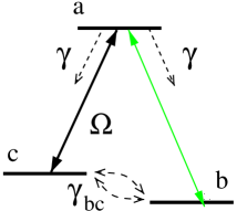
FIG. 1.: Three-level model scheme. The upper level $a$ decays to $b$ and $c$ with decay rate $\gamma$. The relaxation rate between levels $b$ and $c$ is denoted as $\gamma_{bc}$ which is assumed to be small compared with $\gamma$.

The equations of motion for the density matrix elements in a rotating frame are then given by

$${\dot{\rho}}_{ab} = -{\Gamma}_{ab}\rho_{ab}-i\alpha(\rho_{aa}-\rho_{bb})+i\Omega\rho_{cb}$$ (3)

$${\dot{\rho}}_{cb} = -{\Gamma}_{cb}\rho_{cb}-i\alpha\rho_{ca}+i\Omega\rho_{ab}$$ (4)

$${\dot{\rho}}_{ac} = -{\Gamma}_{ac}\rho_{ac}-i\alpha\rho_{bc}-i\Omega(\rho_{aa}-\rho_{cc})$$ (5)

$${\dot{\rho}}_{cc} = -\gamma_{bc}\rho_{cc}+\gamma^{\prime}\rho_{aa}+\gamma_{bc}\rho_{bb}-i\Omega(\rho_{ca}-\rho_{ac})$$ (6)

$${\dot{\rho}}_{aa} = -(\gamma+\gamma^{\prime})\rho_{aa}-i\alpha(\rho_{ab}-\rho_{ba})-i\Omega(\rho_{ac}-\rho_{ca}).$$ (7)

Here we assume that the Rabi frequencies are real, $\Gamma_{ij}$’s are defined as $\gamma_{ij}+i\Delta_{ij}$, where

$$\gamma_{ab} = \gamma_{ac}={1\over 2}(\gamma+\gamma^{\prime}+\gamma_{bc}),\qquad\gamma_{cb}=\gamma_{bc}.$$ (8)

and $\Delta_{ij}$’s are given as $\Delta_{ab}=\omega_{ab}-\nu$, $\Delta_{ac}=\omega_{ac}-\nu_{0}$, and $\Delta_{cb}=\Delta_{ab}-\Delta_{ac}$.

For a weak probe field, first order solution for the off-diagonal density matrix element $\rho_{ab}$ (which governs the absorption of the probe field) can be found in steady state as

$$\rho_{ab}^{(1)}={-i\alpha\over\Gamma_{ab}\Gamma_{cb}+\Omega^{2}}\Big{[}\Gamma_{cb}(\rho_{aa}^{(0)}-\rho_{bb}^{(0)})+{\Omega^{2}\over\Gamma_{ca}}(\rho_{cc}^{(0)}-\rho_{aa}^{(0)})\Big{]}.$$ (9)

where $\rho_{ll}^{(0)}$ is the population in level $l$ in the absence of the probe field. The susceptibility is then written as

$$\chi=\eta\left\{{\rho_{ab}^{(1)}\over\alpha}\right\},$$ (10)

where $\eta$ is given by ${\eta\equiv(3/8\pi)N\gamma\lambda^{3}}$ for the atomic number density $N$ and the wavelength $\lambda$. The effect of the probe field intnsity on the susceptibility is ignored by using the linear approximation [22].

A Optical pumping and population distribution

Let us find the population of each level in the absence of the probe field (i.e. the zeroth order population). Obviously, if the driving field is not turned on, we have $\rho_{aa}=0$ and $\rho_{bb}=\rho_{cc}=1/2$ from Eq. (I). Now as the driving field being turned on, in steady state, we have from Eq. (Ic,e)

$$\rho_{ac}^{(0)} = -{i\Omega\over\Gamma_{ac}}(\rho_{aa}^{(0)}-\rho_{cc}^{(0)}),$$ (11)

$$\rho_{aa}^{(0)} = -{i\Omega\over\gamma+\gamma^{\prime}}(\rho_{ac}^{(0)}-\rho_{ca}^{(0)}).$$ (12)

Let us now assume, for the sake of simplicity, that the decay rate from the level $a$ to $c$ is same as the decay rate from the level $a$ to $b$, i,e. $\gamma^{\prime}=\gamma$ and the driving field detuning is denoted as $\Delta_{0}$. Then, we have $\Gamma_{ac}=\gamma_{ac}+i\Delta_{ac}=(2\gamma+\gamma_{bc})/2+i\Delta_{0}$, and

$$\rho_{ac}^{(0)}-\rho_{ca}^{(0)}={-i2\Omega(\gamma+\gamma_{bc}/2)\over(\gamma+\gamma_{bc}/2)^{2}+\Delta_{0}^{2}}\left(\rho_{aa}^{(0)}-\rho_{cc}^{(0)}\right).$$ (13)

By Eqs. (12) and (13) we obtain

$$\bigg{[}2\gamma+{\Omega^{2}\over X}\bigg{]}\rho_{aa}^{(0)}={\Omega^{2}\over X}\rho_{cc}^{(0)},$$ (14)

where

$$X\equiv{[(\gamma+\gamma_{bc}/2)^{2}+\Delta_{0}^{2}]\over 2(\gamma+\gamma_{bc}/2)}.$$ (15)

Note that Eq. (Id) can be written as

$${\dot{\rho}}_{cc} = -\left(\gamma_{bc}+{\Omega^{2}\over X}\right)\rho_{cc}+\left(\gamma+{\Omega^{2}\over X}\right)\rho_{aa}+\gamma_{bc}\rho_{bb}$$ (16)

Hence using $\rho_{bb}=1-\rho_{aa}-\rho_{cc}$, we obtain the zeroth order population

$$\rho_{aa}^{(0)} = {2\gamma_{bc}\Omega^{2}\over 2D},$$ (18)

$$\rho_{bb}^{(0)} = {4\gamma X\gamma_{bc}+2\gamma_{bc}\Omega^{2}+2\Omega^{2}\gamma\over 2D},$$ (19)

$$\rho_{cc}^{(0)} = {4\gamma X\gamma_{bc}+2\gamma_{bc}\Omega^{2}\over 2D},$$ (20)

where $D\equiv 4\gamma_{bc}\gamma X+3\gamma_{bc}\Omega^{2}+\Omega^{2}\gamma.$ For $\gamma\gg\gamma_{bc}$, these can be simplified as

$$\rho_{aa}^{(0)}-\rho_{cc}^{(0)} \approx -{4\gamma X\gamma_{bc}\over 2D},\quad\rho_{bb}^{(0)}\approx{4\gamma X\gamma_{bc}+2\Omega^{2}\gamma\over 2D},$$ (21)

where

$$X \approx {\gamma^{2}+\Delta_{0}^{2}\over 2\gamma},\qquad D\approx 4\gamma_{bc}\gamma X+\Omega^{2}\gamma.$$ (22)

Note that when the driving field is on resonance, the usual EIT condition $\Omega^{2}\gg\gamma_{bc}\gamma$ is equivalent to $\rho_{bb}\approx 1$ in Eq. (21); i.e. a complete optical pumping to the level $b$ is required to achieve EIT.

B Transmission width of EIT

Now let us consider the transmission width under the condition of a resonant driving field. When we have a resonant driving field, i.e. $\Delta_{0}=0$, from Eq. (22). we find $X\approx\gamma/2$ and $D\approx\Omega^{2}\gamma$. Therefore, $\rho_{aa}^{(0)}\approx\rho_{cc}^{(0)}\approx 0$ and $\rho_{bb}^{(0)}\approx 1$, i.e. all the populations are in the level $b$. As is discussed in the previous section, the condition $\Omega^{2}\gg\gamma_{bc}\gamma$ leads to a complete optical pumping in the homogeneously broadened case.

Eqs. (9,10) then yield

$$\chi = {\eta(-i)\Gamma_{cb}(-1)\over\Gamma_{ab}\Gamma_{cb}+\Omega^{2}}.$$ (23)

Since $\Gamma_{ab}\approx\gamma+i\Delta$ and $\Gamma_{cb}=\gamma_{bc}+i\Delta$, we have

$$\chi = {\eta i\over Z}(\gamma_{bc}+i\Delta)\bigg{[}(\Omega^{2}-\Delta^{2})-i\Delta\gamma\bigg{]},$$ (24)

where $Z=(\Omega^{2}-\Delta^{2})+\Delta^{2}\gamma^{2}$. Hence, the imaginary part is obtained as

$$\chi^{\prime\prime} = {\eta\over Z}\bigg{[}\gamma_{bc}(\Omega^{2}-\Delta^{2})+\Delta^{2}\gamma\bigg{]}.$$ (25)

Since the maximum of $\chi^{\prime\prime}$ is $1/\gamma$ at $\Delta\approx\Omega$, we may define $\Gamma_{EIT}$, the half width of EIT as $\chi^{\prime\prime}(\Delta=\Gamma_{EIT})=1/2\gamma$, which gives

$$\Delta^{4}-\Delta^{2}(2\Omega^{2}+\gamma^{2})+\Omega^{4}=0,$$ (26)

and the solution is

$$\Delta^{2}={\gamma^{2}\over 2}\bigg{[}2s+1\pm\sqrt{4s+1}\bigg{]},$$ (27)

where $s=\Omega^{2}/\gamma^{2}$. Hence for $s\gg 1$ we have

$$\Delta^{2} \approx \gamma^{2}(s+\sqrt{s})$$ (28)

$$\Rightarrow\Delta \approx \pm~{}\Omega\pm{\gamma\over 2},$$ (29)

which shows that the absorption peaks are at $\pm\Omega$ with full width $\gamma$ and the half width of transmission is obtained as

$$\Gamma_{EIT} \approx \Omega-{\gamma\over 2}.$$ (30)

On the other hand, for $s\ll 1$ we have

$$\Delta^{2} \approx {\gamma^{2}\over 2}\bigg{[}2s+1\pm\left(1+2s-2s^{2}\right)\bigg{]}.$$ (31)

Therefore,

$$\Longrightarrow~{}~{}~{}~{}~{}~{}\Delta \approx \pm\left(\gamma+{\Omega^{2}\over\gamma}\right),\qquad\pm{\Omega^{2}\over\gamma}$$ (32)

Hence, when $\Omega\ll\gamma$, we have the absorption profile showing a whole envelope with half width $\gamma+\Omega^{2}/\gamma$, and at the center there exists a transmission line with its half width as

$$\Gamma_{EIT}\sim\Omega^{2}/\gamma.$$ (33)

We note that under the EIT condition $\Omega^{2}\gg\gamma\gamma_{bc}$, $\Gamma_{EIT}$ cannot be smaller than $\gamma_{bc}$.

II Inhomogeneouly Broadened System

Now if the system is Doppler broadened, for the atoms with velocity $v$, the radiation fields are Doppler shifted as $\nu\rightarrow\nu(1-v/c)=\nu-kv$ for the probe field with $k$ as the component of the wavevector on the propagation axis, and $\nu_{0}\rightarrow\nu_{0}(1-v/c)=\nu_{0}-k^{\prime}v$ for the driving field. Hence, for a Doppler broadened system, we replace $\Delta_{ij}$ as $\Delta_{ab}\rightarrow\Delta_{ab}+kv$ $\Delta_{ac}\rightarrow\Delta_{ac}+k^{\prime}v$, and $\Delta_{cb}\rightarrow\Delta_{cb}+(k-k^{\prime})v$. In the present analysis we assume that the energy difference between the level $b$ and $c$ is small enough so that we have $k^{\prime}\approx k$ and the probe field and the driving field are copropagating such that $(k-k^{\prime})v$ term can be neglected. Hence the atomic polarization should be averaged over the entire velocity distribution such that

$$\chi=\int d(kv)~{}f(kv)~{}\eta\left\{{\rho_{ab}(kv)\over\alpha}\right\},$$ (34)

where $f(kv)$ is the velocity distribution function, and again $\eta$ is given by Eq. (10). We now consider the case where the inhomogeneous line is bigger than any other quantities involved such that $W_{D}\gg\Omega,\gamma\gg\gamma_{bc}$, and the condition $\Omega^{2}\gg\gamma_{bc}\gamma$ is still satisfied.

The population distribution in Eq. (21) is now different for atoms with different velocities. As we mentioned in Sec. II, we then need to replace $\Delta_{0}$ with $\Delta_{0}+k^{\prime}v\approx\Delta_{0}+kv$ for the expression of $X$ in Eq. (22) such that for a resonant driving field ($\Delta_{0}=0$) we have

$$X \approx {\gamma^{2}+(kv)^{2}\over 2\gamma},\qquad D\approx 2\gamma_{bc}[\gamma^{2}+(kv)^{2}]+\Omega^{2}\gamma.$$ (35)

Hence, for the atom with its velocity $v$, $\rho_{ab}(kv)$ can be written

$$\rho_{ab}(kv) = {i\alpha\over Y}{1\over 2D}\Big{[}\Gamma_{cb}(4\gamma X\gamma_{bc}+2\Omega^{2}\gamma)$$ (37)

$$\hskip 40.00006pt-\frac{\Omega^{2}4\gamma X\gamma_{bc}}{\gamma+\gamma_{bc}/2+ikv}\Big{]},$$

where $Y=(\gamma+\gamma_{bc}/2+i\Delta+ikv)(\gamma_{bc}+i\Delta)+\Omega^{2}$. Here we have assumed $k^{\prime}\approx k$ and $(k-k^{\prime})v$ terms can be neglected for the copropagating fields.

A Doppler average using a Lorentzian distribution

We now need to evaluate the expression of susceptibility given in Eq. (34).Normally, the velocity distribution is described by a Gaussian function given by

$$f(kv)=\frac{1}{\sqrt{\pi}ku}\exp\left[{-\frac{(kv)^{2}}{(ku)^{2}}}\right],$$ (38)

where $u=\sqrt{2k_{B}T/M}$ is the most probable speed of the atom given by temperature $T$ and the atomic mass $M$. Then, the full width at half maximum is given as $2W_{D}=2\sqrt{\ln{2}}ku$. However, in our analysis, for the sake of simple analytic expressions, we adopt a Lorentzian distribution of FWHM of $2W_{D}$, instead of a Gaussian distribution, such that

$$f(kv)={W_{D}/\pi\over W_{D}^{2}+(kv)^{2}}.$$ (39)

The two distributions are shown in Fig. 2, and there we see that a Gaussian distribution with the same width (FWHM $2W_{D}$) has its maximum larger than that of Lorentzian distribution by a factor of $\sqrt{\pi\ln{2}}$. Hence, if we multiply the factor $\sqrt{\pi\ln{2}}$ in Eq. (39), the central distribution becomes very similar to that of Gaussian as illustrated in Fig. 2(c).

FIG. 2.: Velocity distribution of FWHM $2W_{D}=100\gamma$ as a function a $kv$ in unit of $\gamma$, with (a) a Gaussian profile of Eq.(38), (b) a Lorentzian profile of Eq.(39), (c) the plot ofr Eq.(39) multiplied by a factor $\sqrt{\pi\ln{2}}$.

In Fig. 3 the absorption profiles are described numerically by using the two different distributions. We note that the two distributions give an almost identical result when the factor $\sqrt{\pi\ln{2}}$ is taken into account, see Fig. 3(c).

FIG. 3.: Absorption profiles ($\chi\prime\prime/\eta$) as a function of probe field detuning ($\Delta$ in unit of $\gamma$) for $2W_{D}=100\gamma$, $\gamma_{bc}=10^{-3}\gamma$, and $\Omega=2\gamma$ using (a), (b), (c) of Fig. 2, respectively.

Now using the distribution of Eq. (39), Eq. (34) may be considered as a contour integration in the complex plane. We find three poles in the the upper half plane at

$$kv = \frac{\Delta(\Omega^{2}-\gamma_{bc}^{2}-\Delta^{2})+i(\Delta^{2}\gamma+\gamma_{bc}^{2}\gamma+\gamma_{bc}\Omega^{2})}{\gamma_{bc}^{2}+\Delta^{2}}\;,$$ (41)

$$\quad iW_{D},\qquad\qquad i\sqrt{\Omega^{2}\gamma\over 2\gamma_{bc}},$$

and two poles in the lower half plane as

$$kv=-iW_{D},\qquad-i\sqrt{\Omega^{2}\gamma\over 2\gamma_{bc}}.$$ (42)

We can see that one pole is from the expression $Y$, two poles ($\pm i\sqrt{\Omega^{2}\gamma/2\gamma_{bc}}$) are from the expression $D$ in Eq. (37), and two poles ($\pm iW_{D}$) are from velocity distribution function [27]. Let us take the contour in the lower half plane and denote

$$\chi=\chi_{1}+\chi_{2},$$ (43)

where $\chi_{i}$’s are the contributions from the two poles at $-iW_{D}$ and $-i\sqrt{\Omega^{2}\gamma/2\gamma_{bc}}$, respectively. For the pole at $kv=-iW_{D}$, we obtain

$$\chi_{1} = {-i\eta\over 2Z_{1}A}\bigg{[}(B_{1}-\Delta^{2})-i\Delta W_{D}\bigg{]}~{}\bigg{[}C_{1}-i\Delta D_{1}\bigg{]},$$ (44)

where $A$ is given by

$$A = -2\gamma_{bc}W_{D}^{2}+\Omega^{2}\gamma,$$ (45)

and

$$Z_{1} = (\gamma_{bc}W_{D}+\Omega^{2}-\Delta^{2})^{2}+\Delta^{2}W_{D}^{2},$$ (46)

$$B_{1} = \gamma_{bc}W_{D}+\Omega^{2},$$ (47)

$$C_{1} = 2\gamma_{bc}W_{D}(\gamma_{bc}W_{D}+\Omega^{2})-2\gamma_{bc}\Omega^{2}\gamma,$$ (48)

$$D_{1} = -2\gamma_{bc}W_{D}^{2}+2\Omega^{2}\gamma.$$ (49)

For the pole at $kv=-i\sqrt{\Omega^{2}\gamma/2\gamma_{bc}}$, we have

$$\chi_{2} = {i\eta\Omega^{2}\gamma W_{D}\over 2Z_{2}Ay}\bigg{[}(B_{2}-\Delta^{2})-i\Delta y\bigg{]}~{}\bigg{[}C_{2}-i\Delta\bigg{]},$$ (50)

where $y=\sqrt{\Omega^{2}\gamma/2\gamma_{bc}}$, and

$$Z_{2} = (\gamma_{bc}y+\Omega^{2}-\Delta^{2})^{2}+\Delta^{2}y^{2},$$ (51)

$$B_{2} = \gamma_{bc}y+\Omega^{2},$$ (52)

$$C_{2} = -\gamma_{bc}+\Omega^{2}/y.$$ (53)

Note that we have assumed $\Omega^{2}\gg\gamma_{bc}\gamma$, $W_{D}\gg\Omega,\gamma\gg\gamma_{bc}$.

B Absorption and dispersion at EIT resonance

The absorption profile is now obtained by the imaginary parts of Eqs.(44, 50) as

$$\chi_{1}^{\prime\prime} = {-\eta\over 2Z_{1}A}\bigg{[}(B_{1}-\Delta^{2})C_{1}-\Delta^{2}W_{D}D_{1}\bigg{]},$$ (54)

$$\chi_{2}^{\prime\prime} = {\eta\Omega^{2}\gamma W_{D}\over 2Z_{2}Ay}\bigg{[}(B_{2}-\Delta^{2})C_{2}-\Delta^{2}y\bigg{]}.$$ (55)

Taking $\Delta=0$, we found

$$\chi_{1}^{\prime\prime}(\Delta=0) = {-\eta\over A}\left[\gamma_{bc}W_{D}-{\gamma_{bc}\Omega^{2}\gamma\over+\gamma_{bc}W_{D}+\Omega^{2}}\right],$$ (56)

$$\chi_{2}^{\prime\prime}(\Delta=0) = {\eta\gamma_{bc}W_{D}\over A}\left[1-{2\gamma_{bc}y\over\gamma_{bc}y+\Omega^{2}}\right],$$ (57)

which gives the minimum value of absorption at the EIT line center as

$$\chi^{\prime\prime}(\Delta=0)={\eta\gamma_{bc}\over\gamma_{bc}W_{D}+\Omega^{2}}\left[{\sqrt{x}\over 1+\sqrt{x}}\right],$$ (58)

where

$$x={\Omega^{2}\gamma\over 2\gamma_{bc}W_{D}^{2}}.$$ (59)

We note that when $x\ll 1$,

$$\left.\chi^{\prime\prime}\right|_{\Delta=0} \Longrightarrow ~{}{\eta\gamma_{bc}\over\gamma_{bc}W_{D}+\Omega^{2}}\sqrt{x}~{}<~{}{\eta\sqrt{x}\over W_{D}}~{}\ll~{}{\eta\over W_{D}},$$ (60)

and when $x\gg 1$,

$$\left.\chi^{\prime\prime}\right|_{\Delta=0} \Longrightarrow ~{}{\eta\gamma_{bc}\over\gamma_{bc}W_{D}+\Omega^{2}}~{}<~{}{\eta\gamma_{bc}\over\Omega^{2}}~{}\ll~{}{\eta\gamma\over W_{D}^{2}}.$$ (61)

In both cases the EIT can be achieved, i.e., $\left.\chi^{\prime\prime}\right|_{\Delta=0}\ll\eta/W_{D}$. Therefore, the condition for EIT is still $\Omega^{2}\gg\gamma\gamma_{bc}$, the same as in the homogeneously broadened system.

One interesting quantity here is the slope of the real part of the susceptibility, which is important in precision magnetometry, and also governs the group velocity of the probe light. From Eqs. (44,50) the real part of the susceptibility is found as

$$\chi_{1}^{\prime} = {-\eta\Delta\over 2Z_{1}A}\bigg{[}W_{D}C_{1}+D_{1}(B_{1}-\Delta^{2})\bigg{]},$$ (62)

$$\chi_{2}^{\prime} = {\eta\Omega^{2}\gamma W_{D}\over 2Z_{2}Ay}\Delta\bigg{[}C_{2}y+(B_{2}-\Delta^{2})\bigg{]},$$ (63)

and its derivative at resonance is given by

$$\left.\frac{\partial\chi_{1}^{\prime}}{\partial\Delta}\right|_{\Delta=0}=-{\eta\gamma\over A},\qquad\left.\frac{\partial\chi_{2}^{\prime}}{\partial\Delta}\right|_{\Delta=0}={\eta\sqrt{2\gamma_{bc}\gamma W_{D}^{2}/\Omega^{2}}\over A}.$$ (64)

Hence, we obtained the slope of $\chi^{\prime}$ at $\Delta=0$ as

$$\left.\frac{d\chi^{\prime}}{d\Delta}\right|_{\Delta=0} = -{\eta\over\Omega^{2}}~{}{\sqrt{x}\over 1+\sqrt{x}}.$$ (65)

Therefore, when $x\gg 1$, it approaches to ${\eta/\Omega^{2}}$ and when $x\ll 1$, it goes as $(\eta/\Omega^{2})\sqrt{x}$. We note that, under the EIT condition $\Omega^{2}\gg\gamma_{bc}\gamma$, $(\eta/\Omega^{2})\sqrt{x}$ is still much larger than $(\eta/\Omega^{2})(\gamma/W_{D})$.

$$\left.\frac{d\chi^{\prime}}{d\Delta}\right|_{\Delta=0} \Longrightarrow ~{}-{\eta\over\Omega}~{}{1\over\sqrt{2\gamma_{bc}\gamma}}\left({\gamma\over W_{D}}\right).$$ (66)

C Transmission width of EIT resonance

In order to estimate the linewidth of EIT we take the same procedure as in Sec. II: First, we find that the maximum of $\chi^{\prime\prime}$ as $\chi_{\rm max}\approx\eta/W_{D}$ at $\Delta\approx\pm\Omega$. Then, we evaluate $\Delta$ which defines $\Gamma_{EIT}$ as

$$\chi^{\prime\prime}(\Delta=\Gamma_{EIT})=\eta/2W_{D}.$$ (67)

By Eq. (55) it readily gives the following equation:

$$\Delta^{4}-{2\gamma_{bc}\Omega^{2}\over\gamma}{2\gamma_{bc}W_{D}^{2}+\Omega^{2}\gamma\over 2\gamma_{bc}W_{D}^{2}}\Delta^{2}-{2\gamma_{bc}\Omega^{2}\over\gamma}{\Omega^{4}\ W_{D}^{2}}=0,$$ (68)

which yields the half width of the EIT for the Doppler broadened system given by

$$\Gamma_{EIT}^{2} = {\gamma_{bc}\over\gamma}~{}\Omega^{2}(1+x)\left[1+\left\{1+{4x\over(1+x)^{2}}\right\}^{1/2}\right],$$ (69)

$$\approx {2\gamma_{bc}\over\gamma}~{}\Omega^{2}(1+x),$$ (70)

where $x={\Omega^{2}\gamma/2\gamma_{bc}W_{D}^{2}}$ given by Eq. (59). Now if we define a saturation intensity as

$$\Omega_{s}^{2}={2\gamma_{bc}W_{D}^{2}\over\gamma},$$ (71)

the linewidth expression can be written as

$$\Gamma_{EIT} \approx \left[\sqrt{2\gamma_{bc}\over\gamma}~{}\Omega\right]\sqrt{1+{\Omega^{2}\over\Omega_{s}^{2}}}$$ (72)

Here we can see that in the limit $\Omega\ll\Omega_{s}$ $\Gamma_{EIT}$ is proportional to the Rabi frequency of the driving field. Such a linewidth was predicted by Feld and Javan in the study of laser induced line narrowing [23]. On the other hand, in the limit $\Omega\gg\Omega_{s}$ $\Gamma_{EIT}$ is proportional to the intensity of the driving field ($\Omega^{2}/W_{D}$). This power broadening feature is shown in Fig. 4.

FIG. 4.: Absorption profile for $2W_{D}=100\gamma$, $\gamma_{bc}=10^{-3}\gamma$. (a) $\Omega=\gamma$, (b) $\Omega=3\gamma$, (c) $\Omega=6\gamma$. Note that $\sqrt{\gamma_{bc}\gamma}\sim 0.03\gamma$ and $\Omega_{s}\sim 4.5\gamma$.

The expression of Eq. (72) shows a reminiscence of power broadening factor in the description of hole burning[28]. In place of the homogeneous linewidth in the expression of hole burning, here we have an effective width which is determined by the spectral packet involved in population trapping [26].

D The role of optical pumping

We have seen that the parameter $x=\Omega/\Omega_{s}$ plays an important role in the case of inhomogeneously broadened medium. Let us here examine the physical meaning of the parameter.

Suppose the system is homogeneously broadened. When the driving is on resonance, the optical pumping rate from the level $c$ is then order of $\Omega^{2}/\gamma$, as given in Eq. (16). A complete optical pumping within the homogeneous linewidth, is then possible if this rate is larger than the pumping from level $b$ to $c$: $\Omega^{2}/\gamma\gg\gamma_{bc}$. This, in turn, gives the EIT condition. When we have the driving field detuned by $\Delta_{0}$, the optical pumping rate decreases by a factor of $\gamma^{2}/(\gamma^{2}+\Delta_{0}^{2})$. Again for a complete optical pumping we need $\Omega^{2}\gamma/[\gamma^{2}+\Delta_{0}^{2}]\gg\gamma_{bc}$.

If we now assume that we have the resonant driving field $\Delta_{0}=0$ again, and, instead, the atoms are moving. Then, for atoms with velocity $v$, the optical pumping rate becomes $\Omega^{2}\gamma/[\gamma^{2}+(kv)^{2}]$. Then, on the average, to have a complete optical pumping in a Doppler broadened system we need to require $\Omega^{2}\gamma/(\gamma^{2}+W_{D}^{2})\gg\gamma_{bc}$, which corresponds to $x\gg 1$ (assuming $W_{D}\gg\gamma$), i.e. $\Omega\gg\Omega_{s}\equiv 2\gamma_{bc}W_{D}^{2}/\gamma$. Hence, the parameter $x=\Omega^{2}/\Omega_{s}^{2}$ represents the degree of saturation in $b\leftrightarrow c$ transition, or the degree of optical pumping from the level $c$ to $b$ within the inhomogeneous linewidth.

III Comparison with an open system description

In this section we examine the case of an open system and show that the result is essentially the same as our model of a closed system. The open system is modeled for the atoms that are coming in and out of the interaction (with the radiation fields) region. Although in such a case all the levels have the same decay rate (say, $\gamma_{bc}$), the upper level can decay much faster than the time of flight through the interaction region (for example, radiative decay or collisional decay). Hence we assume that the lower levels $b$ and $c$ decay with rate $\gamma_{bc}$ and the upper level $a$ decays with rate $\gamma_{a}$ which is much bigger than $\gamma_{bc}$ (see Fig. 5).

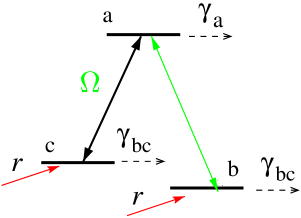
FIG. 5.: Model scheme of the open system. Upper level $a$ decays with rate $\gamma_{a}$ Lower levels $b$ and $c$ decay with the same rate $\gamma_{bc}$. Atoms are pumped at a rate $r$ equally to the lower levels.

Furthermore, for simplicity, we assume that the atoms are coming into the interaction region with a same rate for the lower levels. Under these assumption, the equation of motion for the density matrix elements can be written as

$${\dot{\rho}}_{ab} = -{\Gamma}_{ab}\rho_{ab}-i\alpha(\rho_{aa}-\rho_{bb})+i\Omega\rho_{cb},$$ (74)

$${\dot{\rho}}_{cb} = -{\Gamma}_{cb}\rho_{cb}-i\alpha\rho_{ca}+i\Omega\rho_{ab},$$ (75)

$${\dot{\rho}}_{ac} = -{\Gamma}_{ac}\rho_{ac}-i\alpha\rho_{bc}-i\Omega(\rho_{aa}-\rho_{cc}),$$ (76)

$${\dot{\rho}}_{aa} = -\gamma_{a}\rho_{aa}-i\alpha(\rho_{ab}-\rho_{ba})-i\Omega(\rho_{ac}-\rho_{ca}),$$ (77)

$${\dot{\rho}}_{bb} = r-\gamma_{bc}\rho_{bb}-i\alpha(\rho_{ab}-\rho_{ba})-i\Omega(\rho_{ac}-\rho_{ca}),$$ (78)

$${\dot{\rho}}_{cc} = r-\gamma_{bc}\rho_{cc}-i\Omega(\rho_{ca}-\rho_{ac}).$$ (79)

Here the notations are the same as Eq. (I). Note that now we have $\Gamma_{ac}=(\gamma_{a}+\gamma_{bc})/2+i\Delta_{0}$, which gives

$$X^{\prime}\equiv{[(\gamma_{a}/2+\gamma_{bc}/2)^{2}+\Delta_{0}^{2}]\over 2(\gamma_{a}/2+\gamma_{bc}/2)}.$$ (80)

Again if we assume that $\gamma_{a}\gg\gamma_{bc}$, the populations are found as

$$\rho_{aa}^{(0)}-\rho_{cc}^{(0)} \approx -{\gamma_{bc}\gamma_{a}X^{\prime}\over 2D^{\prime}},\quad\rho_{bb}^{(0)}\approx{\gamma_{bc}\gamma_{a}X^{\prime}+\Omega^{2}\gamma_{a}\over 2D^{\prime}},$$ (81)

where

$$X^{\prime} \approx {(\gamma_{a}/2)^{2}+\Delta_{0}^{2}\over\gamma_{a}},\qquad D^{\prime}\approx\gamma_{bc}\gamma_{a}X^{\prime}+\Omega^{2}\gamma_{a}.$$ (82)

Comparing Eq. (81) with (21), we can see that the population distribution is almost identical to the one for the model of closed system.

Furthermore, the expression for $\rho_{ab}^{(1)}$ is identical to the one for the closed system given in Eq. (9). Let us then recall Eq. (45) saying that $A=-2\gamma_{bc}W_{D}^{2}+\Omega^{2}\gamma$, which is obtained by putting $-iW_{D}$ to $\Delta_{0}$ in the expression of $D$ in Eq. (I A). The sign of $A$ determines whether the crucial parameter $x$ is $>1$ or $<1$. Similarly, here for the open system, when we put $\Delta_{0}=-iW_{D}$, we can define $A^{\prime}$ as $A^{\prime}\approx-\gamma_{bc}W_{D}^{2}+\Omega^{2}\gamma_{a}$ such that we have $x^{\prime}=\Omega\gamma_{a}/\gamma_{bc}W_{D}^{2}$ as the parameter which plays the same role as $x$ in Eq. (22). Hence, by replacing $\gamma_{a}\Rightarrow 2\gamma$, we have the open system description almost identical to the description for our model scheme of the closed system A detailed analysis of the open system will be presented elsewhere [29].

IV Summary

In this paper, we have studied the transmission width of EIT in a three-level $\Lambda$ system. The Doppler averaged susceptibility is found by using a Lorentzian velocity distribution rather than the Gaussian distribution. Then we have shown the requirement for achieving EIT, and the analytic expression of the EIT linewidth. The saturation intensity $\Omega_{s}^{2}$ defines the degree of optical pumping as $\Omega^{2}/\Omega_{s}^{2}$, and represents the condition under which the broadening is either linear or quadratic in the Rabi frequency of the driving field.

REFERENCES

• [1] See, for example, E. Arimondo: Progress in Optics XXXV edited by E. Wolf, p257 (Elsevier Science, Amsterdam, 1996)
• [2] S.E. Harris: Physics Today, 50 (7), 36 (1997)
• [3] O.A. Kocharovskaya and Ya.I. Khanin: Sov. Phys.  JETP Lett. 63, 945, (1986)
• [4] K.J. Boller, A. Imamog̃lu, and S.E. Harris: Phys. Rev. Lett. 66, 2593 (1991); J.E. Field, and K.H. Hahn, and S.E. Harris: Phys. Rev. Lett. 67, 3062 (1991)
• [5] S.E. Harris, J.E. Field, A. Imamoğlu: Phys. Rev. Lett. 64, 1107 (1990)
• [6] K. Hakuta, L. Marmet, B.P. Stoicheff: Phys. Rev. Lett. 66, 596 (1991)
• [7] S.E. Harris and L.V. Hau: Phys. Rev. Lett. 82, 4611 (1999)
• [8] S.E. Harris, J.E. Field, and A. Kasapi: Phys. Rev A 46, R29 (1992)
• [9] M. Xiao, Y.Q. Li, S.Z. Jin, and J. Gea-Banacloche: Phys. Rev. Lett. 74, 666 (1995)
• [10] O. Schmidt, R. Wynands, Z. Hussein, and D. Meschede: Phys. Rev. A 53, R27 (1996)
• [11] L.V. Hau, S.E. Harris, Z. Dutton, and C.H. Behroozi: Nature 397, 594 (1999)
• [12] M.M. Kash, V.A. Sautenkov, A.S. Zibrov, L. Hollberg, G.R. Welch, M.D. Lukin, Y. Rostovtsev, E.S. Fry, and M.O. Scully: Phys. Rev. Lett. 82, 5229 (1999)
• [13] D. Budker, D.F. Kimball, S.M. Rochester, and V.V Yashchuk: Phys. Rev. Lett. 83, 1767 (1999)
• [14] O. Kocharovskaya, Y. Rostovtsev, and M.O. Scully: Phys. Rev. Lett. 86, 628 (2001)
• [15] M.O. Scully and M. Fleischhauer: Phys. Rev. Lett. 69, 1360 (1992); M. Fleischhauer and M.O. Scully: Phys. Rev. A 49, 1973 (1994)
• [16] S. Brandt, A. Nagel, R. Wynands, and D. Meschede: Phys. Rev. A 56, R1063 (1997); A. Nagel, L.Graf, A.Naumov, E.Mariotti, V.Biancalana, D.Meschede, and R.Wynands: Europhys. Lett. 44, 31 (1998)
• [17] M.D. Lukin, M. Fleischhauer, A.S. Zibrov, H.G. Robinson, V.L. Velichansky, L. Hollberg, and M.O. Scully: Phys. Rev. Lett. 79, 2959 (1997)
• [18] D. Budker, V. Yashchuk, and M. Zolotorev: Phys. Rev. Lett. 81, 5788 (1998)
• [19] J. Gea-Banacloche, Y.Q. Li, S.Z. Jin, and M. Xiao: Phys. Rev. A 51, 576 (1995)
• [20] A. Karawajczyk and J. Zakrzewski: Phys. Rev. A 51, 830 (1995)
• [21] D. Wang and J. Gao: Phys. Rev. A ibid. 52, 3201 (1995)
• [22] A.V. Taichenachev, A.M. Tumaikin, and V.I. Yudin: JETP Lett. 72, 173 (2000)
• [23] M.S. Field and A. Javan: Phys. Rev. 177, 540 (1969)
• [24] T.W. Hänsch and P.E. Toschek: Z. Phys. 236, 213 (1970)
• [25] T. Popova, A. Popov, and S. Ravtian, and R. Sokolovskii: Zh. Eksp. Teor. Fiz. 57, 850 (1969) [Sov. Phys. JETP Lett. 30, 466 (1970)]
• [26] A. Javan, O. Kocharovskaya, H. Lee, and M.O. Scully: (to be published)
• [27] Note that the expression $-\Omega^{2}4\gamma X\gamma_{bc}/(\gamma+\gamma_{bc}/2+ikv)$ in Eq. (37) does not have a pole as we recall the original form of $X$ in Eq. (15).
• [28] See, for example, A. Yariv: Quantum Electronics (Wiley, New York, 1989)
• [29] Y. Rostovtsev I. Protsenko, H. Lee, and A. Javan: (to be published).