Towards a third-order topological invariant for magnetic fields

Abstract

An expression for a third-order link integral of three magnetic fields is presented. It is a topological invariant and therefore an invariant of ideal magnetohydrodynamics. The integral generalizes existing expressions for third-order invariants which are obtained from the Massey triple product, where the three fields are restricted to isolated flux tubes. The derivation and interpretation of the invariant shows a close relationship with the well-known magnetic helicity, which is a second-order topological invariant. Using gauge fields with an $SU(2)$ symmetry, helicity and the new third-order invariant originate from the same identity, an identity which relates the second Chern class and the Chern-Simons three-form. We present an explicit example of three magnetic fields with non-disjunct support. These fields, derived from a vacuum Yang-Mills field with a non-vanishing winding number, possess a third-order linkage detected by our invariant.

,

1 Introduction

The topological structure of magnetic fields is an important subject in plasma physics. There, among other issues, it is related to the problem of stability of a plasma and to its energy content. Fields with an enormous wealth of entangled, braided or knotted field lines exist for example in the solar atmosphere. Note that the topological complexity of these solar magnetic fields is only revealed, if first, one takes into account that the observed loops anchored in the photosphere are closed by subphotospheric fields, and second, that already simple toroidal equilibria contain many different knotted and linked field lines. The simplest examples are the so called torus knots, which are formed by field lines where the quotient of the number of windings around the core and the torus axis is rational.

In general, magnetic fields in plasmas are not static, but evolve due to the motion of the plasma. The evolution of solar as well as most astrophysical magnetic fields is given in good approximation by the induction equation of ideal magnetohydrodynamics (IMHD)

$$\frac{\partial}{\partial t}{\bf B}-\nabla\times({\bf v}\times{\bf B})=0,$$ (1)

which shows that the field can be considered as frozen-in with respect to the plasma velocity ${\bf v}$. The approximation of IMHD which leads to this law is valid as long as the evolution does not lead to small scale structures, e.g. thin current sheets.

The ideal induction equation guarantees the conservation of the topology of field lines under the flow of ${\bf v}$, i.e. every linkage or knottedness of magnetic flux is preserved. Mathematically speaking, the flow of ${\bf v}$ is a differentiable isotopy of the space under consideration. It maps the field lines of ${\bf B}$ at time $t_{0}$ to a topologically equivalent set of field lines for any later time $t>t_{0}$. Let us note that, following the usual terminology in plasma physics, the term ‘topological equivalent’ is used here in the sense of a diffeomorphic isotopy.

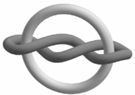
Figure 1: The Borromean rings (left) and the Whitehead link (right).

In order to describe the structure of magnetic fields, it is desirable to have measures of complexity. These measures should be topological, i.e. they should be invariant under an arbitrary isotopy of the magnetic field, and therefore invariant under the ideal induction equation. An example of a topological measure for magnetic fields is the magnetic helicity, a quantity which has attracted a great deal of attention in recent years (see e.g. Brown et al1999). Magnetic helicity, which measures the linkage of magnetic flux, is only a lowest order topological measure. It fails for instance to detect the interlocking of magnetic flux tubes in form of the Borromean rings or the Whitehead link (see Figure 1). The total magnetic helicity of these configurations vanishes just as it does for three or two unlinked flux tubes. Both configurations must possess a higher order linkage or knottedness of magnetic flux which is not detected by magnetic helicity. This naturally raises the question whether corresponding higher order measures similar to magnetic helicity exist which are sensitive to these linkages. Here we would like to remark that the configurations shown in Figure 1 are highly idealized. In any real plasma we would not find this pure linkage but a mixture of different types of linkages, each of which is to be measured by a different integral.

In knot theory different invariants are known which distinguish e.g. the Borromean rings or the Whitehead link from unlinked rings. The problem is that invariants used in physical applications, e.g. in magnetohydrodynamics, should be expressed in terms of observable quantities, in our setting in terms of the magnetic field ${\mathbf{B}}$. Up to now only the helicity, which is related to the Gauß  linking number, has been formulated as an invariant for magnetic fields in a satisfactory manner. As was recognized first by Monastyrsky and Sasorov (1987) and independently by Berger (1990) and Evans and Berger (1992), the link invariants based on so-called higher Massey products (see Massey 1958, 1969, Kraines 1966, Fenn 1983) can be written as invariants applicable to magnetic flux tubes. Similar to helicity, they only involve the magnetic fields and can be expressed as volume integrals over the space in consideration. Their disadvantage is that their usage is restricted to magnetic fields confined to isolated flux tubes. In addition, these flux tubes must not possess a linkage lower than the linkage which is measured.

In this paper we present a generalized third-order invariant for three magnetic fields not confined to isolated flux tubes. In the case of isolated flux tubes this invariant coincides with the invariant known from the Massey triple product. Using gauge fields in the context of an $SU(2)$ symmetry, the generalized invariant can be shown to originate from the same equation as helicity. Therefore, we will first recapitulate some basic facts about magnetic helicity before we turn to our main subject, the third-order link invariant.

2 Magnetic helicity

Magnetic helicity of a field ${\mathbf{B}}$ with arbitrary vector potential ${\mathbf{A}}$ is defined as

$$H({\mathbf{B}})=\int_{V}{\mathbf{A}}\cdot{\mathbf{B}}\,\mbox{d}^{3}\!x\,,\quad\quad\quad{\mathbf{B}}\cdot{\mathbf{n}}|_{\partial V}=0,$$ (2)

which can readily be shown to be gauge invariant if no magnetic flux crosses the boundary of the volume. Since it is quadratic in magnetic flux it is often referred to as a second-order topological invariant. Magnetic helicity measures the total mutual linkage of magnetic flux. This interpretation can be motivated if we envisage a simple system of two isolated and closed flux tubes $U_{1}$ and $U_{2}$ with vanishingly small cross-section. The latter condition ensures that the (self-)helicities of the flux tubes vanish. Moffatt (1969) has shown that for this configuration the helicity integral yields $H({\mathbf{B}})=2\,\phi_{1}\phi_{2}\,\mbox{lk}(U_{1},U_{2})$, where $\mbox{lk}(U_{1},U_{2})$ is the Gauß  linking number (Gauß 1867) of the two tubes and where $\phi_{i}$ is the magnetic flux in the tube $U_{i}$. Introducing an asymptotic linking number, Arnol’d (1974) was able to extend this interpretation to the generic case where field lines are not necessarily closed (see also Arnol’d & Khesin 1998, Part III, §4).

Similar to helicity we can introduce the more general cross-helicity of two magnetic fields ${\mathbf{B}}_{1}$ and ${\mathbf{B}}_{2}$. For a simply connected volume $V$ and provided that ${\mathbf{B}}_{1}\cdot{\mathbf{n}}|_{\partial V}={\mathbf{B}}_{2}\cdot{\mathbf{n}}|_{\partial V}=0$ we define

$$H({\mathbf{B}}_{1},{\mathbf{B}}_{2}):=\int_{V}{\mathbf{A}}_{1}\cdot{\mathbf{B}}_{2}\,\mbox{d}^{3}\!x=\int_{V}{\mathbf{B}}_{1}\cdot{\mathbf{A}}_{2}\,\mbox{d}^{3}\!x.$$ (3)

The boundary conditions ensure that this is again a gauge invariant quantity. To see that the two integrals on the right-hand side are equivalent, note that they differ only by a surface integral $\int({\mathbf{A}}_{1}\times{\mathbf{A}}_{2})\cdot{\bf n}\,\mbox{d}^{2}\!x$. This can be shown to vanish using the equivalence of ${\mathbf{B}}_{i}\cdot{\mathbf{n}}|_{\partial V}=0$ with ${\mathbf{A}}_{i}\times{\mathbf{n}}|_{\partial V}=0$ in a certain gauge and for a simply connected volume $V$, as proved in A. Since both integrals are gauge invariant this proves the equality for any gauge.

$H({\mathbf{B}}_{1},{\mathbf{B}}_{2})$ measures purely the cross linkage of flux among the two fields. Applied to our system of two isolated closed flux tubes with fields ${\mathbf{B}}_{1}+{\mathbf{B}}_{2}={\mathbf{B}}$ in the corresponding tubes this invariant yields

$$H({\mathbf{B}}_{1},{\mathbf{B}}_{2})=2\,\phi_{1}\phi_{2}\,\mbox{lk}(U_{1},U_{2}),$$ (4)

which is now valid without the assumption of vanishingly small tube cross-sections.

The significance of magnetic helicity arises from the fact that it is invariant in IMHD. Using merely the homogeneous Maxwell equations we obtain

$${\partial}_{t}({\mathbf{A}}\cdot{\mathbf{B}})+\nabla\cdot\left(A_{0}{\mathbf{B}}+{\mathbf{E}}\times{\mathbf{A}}\right)\,=\,-2{\mathbf{E}}\cdot{\mathbf{B}},$$ (5)

which describes the time evolution of helicity density ${\mathbf{A}}\cdot{\mathbf{B}}$. Here $A_{0}$ is the electric potential and ${\mathbf{E}}$ the electric field. The term $A_{0}{\mathbf{B}}+{\mathbf{E}}\times{\mathbf{A}}$ is to be interpreted as a helicity current, and $-2{\mathbf{E}}\cdot{\mathbf{B}}$ as a source term. In an ideal plasma, i.e. with ${\mathbf{E}}+{\mathbf{v}}\times{\mathbf{B}}=0$, the source term vanishes and the helicity current can be written as

$$A_{0}{\mathbf{B}}+{\mathbf{E}}\times{\mathbf{A}}=A_{0}{\mathbf{B}}+{\mathbf{v}}\left({\mathbf{A}}\cdot{\mathbf{B}}\right)-{\mathbf{B}}\left({\mathbf{A}}\cdot{\mathbf{v}}\right).$$ (6)

Therefore equation (5) takes the form:

$${\partial}_{t}\left({\mathbf{A}}\cdot{\mathbf{B}}\right)+\nabla\cdot\left({\mathbf{v}}\left({\mathbf{A}}\cdot{\mathbf{B}}\right)\right)=\nabla\cdot\left(\chi{\mathbf{B}}\right),$$ (7)

with $\chi=-A_{0}+{\mathbf{A}}\cdot{\mathbf{v}}$. Elsasser (1956) already noticed that a particular gauge can be found such that $\chi=0$. Using either this gauge or an arbitrary gauge together with the boundary condition ${\mathbf{B}}\cdot{\mathbf{n}}\big{|}_{{\partial}V}=0$ this last equation implies the conservation of helicity in a comoving volume for an ideal plasma, since

$$\frac{\mbox{d}}{\mbox{d}t}\int\limits_{V}{\mathbf{A}}\cdot{\mathbf{B}}\,\mbox{d}^{3}\!x=\int\limits_{V}{\partial}_{t}\left({\mathbf{A}}\cdot{\mathbf{B}}\right)+\nabla\cdot\left({\mathbf{v}}\left({\mathbf{A}}\cdot{\mathbf{B}}\right)\right)\,\mbox{d}^{3}\!x=\int\limits_{{\partial}V}\chi{\mathbf{B}}\cdot{\mathbf{n}}\,\mbox{d}^{2}\!x\,=\,0.$$ (8)

The invariance of integral (2) was first stated by Woltjer (1958).

3 A third-order invariant from the Chern-Simons three-form

In this section we construct a third-order invariant which, under conditions specified below, yields an invariant for three magnetic fields. The derivation is based on some basic knowledge in differential geometry found e.g. in Frankel (1997).

We have noted before that equation (5) can be derived purely from the homogeneous Maxwell equations. Written in differential forms it reads

$$\mbox{d}(A\wedge\mbox{d}A)=F\wedge F,$$ (9)

where $A$ is the one-form potential of the field $F$. The right-hand side of this equation is one of two (pseudo-) scalar Lorentz invariants that can be constructed from the field tensor. We can interpret this equation as a special case of a general result in the theory of Chern forms, namely the exactness of the second Chern form

$$\mbox{d}\,tr(A\wedge\mbox{d}A-iq\frac{2}{3}A\wedge A\wedge A)=tr(F\wedge F).$$ (10)

In this equation $A$ and $F$ are a matrix valued one- and two-form. To be more precise they take their values in the Lie-Algebra ${\mathfrak{g}}$ of the structure group. In Yang-Mills theory this is the symmetry group of the interaction under consideration, with coupling constant $q$. On the vector space ${\mathfrak{g}}$ the trace defines a natural scalar product. For $\omega$, $\theta\in{\mathfrak{g}}$, $\tr(\omega\wedge\theta)=\omega_{ij}\wedge\theta_{ji}$, where the indices denote matrix components.

Equation (10) holds for an arbitrary, not necessarily Abelian, field strength $F=\mbox{d}A-iqA\wedge A$. The three-form on the left-hand side is known as the Chern-Simons three-form. For the case of electrodynamics, i.e. for the Abelian structure group $U(1)$, $F$ is given by $F=\mbox{d}\,A$, since $A\wedge A$ vanishes and equation (10) reduces to (9). In the non-Abelian case equation (10) splits into a real and imaginary part

$$\tr(\mbox{d}A\wedge\mbox{d}A)=\mbox{d}\tr(A\wedge\mbox{d}A),$$ (11)

$$2\tr(A\wedge A\wedge\mbox{d}A)=\mbox{d}\tr(\frac{2}{3}A\wedge A\wedge A).$$ (12)

As we will see in the following a third-order invariant can be derived from identity (12) for the special case of the structure group $SU(2)$.

Working with an $SU(2)$ structure group it is appropriate to choose the Pauli matrices $\sigma_{i}$, $i$=$1,2,3$, as a basis for the Lie Algebra $su(2)$. All results, however, are independent of this choice. The gauge potential $A$ and field strength $F$ now have three components

$$A=\sigma_{i}A^{i},\qquad\qquad F=\sigma_{i}F^{i},$$ (13)

where the summation convention over repeated indices is assumed. Let us note that in the following we will refer to these fields as Yang-Mills fields, although they do not necessarily satisfy the Yang-Mills equation. Using the identities for Pauli matrices

$$\sigma_{j}\sigma_{k}=i\;\epsilon_{jkl}\;\sigma_{l}+\delta_{jk}\mathbf{1}\qquad\mbox{and}\qquad\sigma_{j}\,\sigma_{k}\,\sigma_{l}=i\,\epsilon_{jkl}\mathbf{1},$$ (14)

equations (11) and (12) read

$$\mbox{d}A^{i}\wedge\mbox{d}A^{i}=\mbox{d}(A^{i}\wedge\mbox{d}A^{i}),$$ (15)

$$\epsilon_{ijk}\,\mbox{d}A^{i}\wedge A^{j}\wedge A^{k}=\frac{1}{3}\,\mbox{d}(\epsilon_{ijk}A^{i}\wedge A^{j}\wedge A^{k}).$$ (16)

If we now interpret the three components of the Yang-Mills potential $A$ as three independent potentials of three electromagnetic fields $F_{EM}^{i}=\mbox{d}A^{i}$, the first identity states the helicity conservation (in IMHD) for the sum of the self-helicities of the three individual fields $F_{EM}^{i}$, similar to the electrodynamic case. The second identity is new. For convenience we introduce the two-form $G^{1}=A^{2}\wedge A^{3}$, here on $I\!\!M^{4}$, and cyclic permutations of it. Then we can write the second identity as

$$\frac{1}{3}\mbox{d}(A^{i}\wedge G^{i})=F_{EM}^{i}\wedge G^{i}.$$ (17)

To complete the analogy of this equation with equation (5) we have to rewrite it in the language of three-vectors. Therefore we represent the one-form $A^{i}$ by the time component $A_{0}^{i}$ and the three-vector ${\mathbf{A}}^{i}$ of the corresponding four-vector. The two-form $G^{1}$ is identified with the vector pair $({\mathbf{G}}_{E}^{1},{\mathbf{G}}_{B}^{1})=(A_{0}^{3}{\mathbf{A}}^{2}-A_{0}^{2}{\mathbf{A}}^{3},{\mathbf{A}}^{2}\times{\mathbf{A}}^{3})$, equivalent to the identification of $F_{EM}$ with the three-vector pair (${\mathbf{E}}$,-${\mathbf{B}}$). Cyclic permutations immediately lead to corresponding pairs for $G^{2}$ and $G^{3}$. Using these conventions, the left- and right-hand side of equation (17) read respectively

$$\frac{1}{3}\mbox{d}(A^{i}\wedge G^{i}) =-\frac{1}{3}\left({\partial}_{t}({\mathbf{A}}^{i}\cdot{\mathbf{G}}_{B}^{i})+\nabla\cdot(A_{0}^{i}{\mathbf{G}}_{B}^{i}+{\mathbf{A}}^{i}\times{\mathbf{G}}_{E}^{i})\right){\mbox{vol}^{4}}$$

$$=-\left({\partial}_{t}({\mathbf{A}}^{1}\cdot{\mathbf{G}}_{B}^{1})+\nabla\cdot(A_{0}^{i}{\mathbf{G}}_{B}^{i})\right){\mbox{vol}^{4}}$$

and

$$F_{EM}^{i}\wedge G^{i}=({\mathbf{E}}^{i}\cdot{\mathbf{G}}_{B}^{i}-{\mathbf{B}}^{i}\cdot{\mathbf{G}}_{E}^{i}){\mbox{vol}^{4}}=({\mathbf{E}}^{i}\cdot{\mathbf{G}}_{B}^{i}-A_{0}^{i}\nabla\cdot{\mathbf{G}}_{B}^{i}){\mbox{vol}^{4}}.$$

Thus, identity (17) is equivalent to

$${\partial}_{t}({\mathbf{A}}^{1}\cdot{\mathbf{G}}_{B}^{1})+\nabla\cdot(A_{0}^{i}{\mathbf{G}}_{B}^{i})=-{\mathbf{E}}^{i}\cdot{\mathbf{G}}_{B}^{i}+A_{0}^{i}\nabla\cdot{\mathbf{G}}_{B}^{i},$$ (18)

which shows a similar structure as equation (5) in the case of helicity. It describes the time evolution of the density ${\mathbf{A}}^{1}\cdot{\mathbf{A}}^{2}\times{\mathbf{A}}^{3}$ with its current $A_{0}^{i}{\mathbf{G}}_{B}^{i}$ and source term $-{\mathbf{E}}^{i}\cdot{\mathbf{G}}_{B}^{i}+A_{0}^{i}\nabla\cdot{\mathbf{G}}_{B}^{i}$. This is the basis for the following theorem.

Theorem: Let ${\mathbf{B}}^{1}$, ${\mathbf{B}}^{2}$ and ${\mathbf{B}}^{3}$ be three magnetic fields with potentials ${\mathbf{A}}^{i}$ satisfying ${\mathbf{E}}^{i}+{\mathbf{v}}\times{\mathbf{B}}^{i}=0$. The integral over a volume $V\subset I\!\!R^{3}$

$$H^{(3)}({\mathbf{B}}^{1},{\mathbf{B}}^{2},{\mathbf{B}}^{3}):=\int_{V}{\mathbf{A}}^{1}\cdot{\mathbf{A}}^{2}\times{\mathbf{A}}^{3}\,\mbox{d}^{3}\!x$$ (19)

is a gauge invariant, conserved quantity, if

1. the potentials obey $\nabla\cdot({\mathbf{A}}^{i}\times{\mathbf{A}}^{j})=0$ for all $i,j=1,2,3$,

2. the potentials obey the boundary condition ${\mathbf{A}}^{i}\times{\mathbf{n}}|_{{\partial}V}=0$ for ${\mathbf{n}}$ being the normal vector to the boundary of the integration volume $V$.

Proof: Let us first remark that condition (2) of the theorem implies ${\mathbf{B}}^{i}\cdot{\mathbf{n}}|_{{\partial}V}=0$ as shown in A. It is therefore consistent with condition (1) since $0=({\mathbf{B}}^{i}\cdot{\mathbf{A}}^{j}-{\mathbf{A}}^{i}\cdot{\mathbf{B}}^{j})|_{{\partial}V}=\nabla\cdot({\mathbf{A}}^{i}\times{\mathbf{A}}^{j})|_{{\partial}V}$. Moreover, we show in A that for a simply connected volume with ${\mathbf{B}}^{i}\cdot{\mathbf{n}}|_{{\partial}V}=0$ condition (2) can always be satisfied. In order to prove the invariance of $H^{(3)}$ we observe that in an ideal dynamics equation (18) can be written as

$${\partial}_{t}({\mathbf{A}}^{1}\cdot{\mathbf{A}}^{2}\times{\mathbf{A}}^{3})\,+\, \nabla\cdot\left({\mathbf{v}}({\mathbf{A}}^{1}\cdot{\mathbf{A}}^{2}\times{\mathbf{A}}^{3})\right)=$$

$$\nabla\cdot\left(\frac{1}{3}{\mathbf{v}}({\mathbf{A}}^{i}\cdot{\mathbf{G}}_{B}^{i})-A_{0}^{i}{\mathbf{G}}_{B}^{i}\right)+(A_{0}^{i}-{\mathbf{A}}^{i}\cdot{\mathbf{v}})\nabla\cdot{\mathbf{G}}_{B}^{i},$$

where the last term vanishes due to condition (1).

Integrating over the volume $V$ yields the total time derivative of $H^{(3)}$ on the left-hand side, while the right-hand side can be converted into a surface integral, analogous to equation (8) in the case of helicity. The surface integral vanishes since condition (2) of the theorem implies ${\mathbf{G}}_{B}^{i}=0$ on the boundary of the volume $V$. This, together with the gauge invariance of $H^{(3)}$ shown in B, completes the proof.

4 Interpretation of the invariant

It is interesting to note that the new third-order invariant comes on an equal footing as the conservation of helicity, since both invariants where derived from the same identity (10). However, contrary to the conservation of helicity, the third-order integral cannot be applied to a single magnetic field, but requires a triplet of fields. Thus we have to interpret this integral in the sense of the cross-helicity rather than the total helicity. A forthcoming paper will deal with the question of how a single magnetic field might be split into a triplet of fields with the required properties $\nabla\cdot{\mathbf{G}}^{i}=0$, thereby linking the given cross third-order invariant and a total third-order invariant.

There is another way of looking at the new third-order invariant. By writing

$$H^{(3)}({\mathbf{B}}^{1},{\mathbf{B}}^{2},{\mathbf{B}}^{3})=\int_{V}{\mathbf{A}}^{1}\cdot{\mathbf{G}}_{B}^{1}\,\mbox{d}^{3}\!x=H({\mathbf{B}}^{1},{\mathbf{G}}_{B}^{1})\ ,$$ (20)

the integral is to be interpreted as the cross-helicity of the two divergence-free fields ${\mathbf{B}}^{1}$ and ${\mathbf{G}}_{B}^{1}$. Note that the boundary conditions for the cross-helicity, namely ${\mathbf{B}}^{1}\cdot{\mathbf{n}}=0$ and ${\mathbf{G}}_{B}^{1}\cdot{\mathbf{n}}=0$, are fulfilled due to condition (2) of the theorem. From this new interpretation the condition $\nabla\cdot{\mathbf{G}}_{B}^{1}=0$ is an obvious requirement analogous to $\nabla\cdot{\mathbf{B}}=0$. Furthermore, the symmetry of $H^{(3)}$ leads to

$$H({\mathbf{B}}^{1},{\mathbf{G}}_{B}^{1})=H({\mathbf{B}}^{2},{\mathbf{G}}_{B}^{2})=H({\mathbf{B}}^{3},{\mathbf{G}}_{B}^{3}),$$ (21)

which reveals the additional conditions $\nabla\cdot{\mathbf{G}}_{B}^{2}=0$ and $\nabla\cdot{\mathbf{G}}_{B}^{3}=0$. Let us note that this interpretation does not simplify the direct calculation of the third-order invariant. It is still necessary to determine the fields ${\mathbf{G}}_{B}^{i}$ which are not independent of the chosen representatives ${\mathbf{A}}^{i}$.

Third-order linking integrals for magnetic fields have been constructed from the Massey triple product already by Monastyrsky and Sasorov (1987), Berger (1990) and also Ruzmaikin and Akhmetiev (1994). However, these constructions are limited to cases where the three fields are confined to three isolated and mutually unlinked flux tubes with disjunct support. It is in fact easy to see that for this special case their invariants coincide with the integral (19) given above. An explicit proof is given in C. In particular, it is worth noting that for fields with mutually disjunct support the condition $\nabla\cdot{\mathbf{G}}^{i}_{B}=0$ implies that the cross-helicity of all pairs of fields vanishes, i.e. their flux tubes have to be mutually unlinked.

For a set of three arbitrary magnetic fields $\nabla\cdot{\mathbf{G}}^{i}_{B}=0$ cannot always be satisfied. To show that there are examples for which this can be satisfied, beyond the cases of three fields with mutually disjunct support, we give an explicit example in the next section.

5 Example of three magnetic fields with a third-order linkage

In this section we want to give an example of three magnetic fields not confined to flux tubes, which firstly allow for one-form potentials that obey $\mbox{d}(A^{i}\wedge A^{j})=0$ and where secondly the integral invariant (19) yields a non-trivial result. The existence of such an example proves that the new invariant is indeed a generalization of the third-order invariant derived from a Massey triple product which was applicable merely to unlinked flux tubes. The fields we construct show an extraordinary high symmetry. For this reason they are interesting in their own right.

The idea to construct three fields $A^{i}$ on $I\!\!R^{4}$ which obey $\mbox{d}(A^{i}\wedge A^{j})=0$ comes from Yang-Mills theory: An $SU(2)$ Yang-Mills field

$$F=\mbox{d}A-iqA\wedge A$$ (22)

can, in view of equation (13) and the identities for Pauli matrices (14), be written as

$$F^{i}=\mbox{d}A^{i}+q\,\epsilon_{ijk}A^{j}\wedge A^{k}.$$ (23)

By taking the exterior derivative of $F$,

$$\mbox{d}F^{i}=q\,\epsilon_{ijk}\mbox{d}(A^{j}\wedge A^{k}),$$ (24)

we immediately observe that $\mbox{d}F=0$ is a sufficient condition for all $\mbox{d}(A^{i}\wedge A^{j})$ to vanish. In the special case of a vacuum Yang-Mills field, i.e. $F=0$, the requirement $\mbox{d}F=0$ is trivially fulfilled. If we now reinterpret the three components of the Yang-Mills potential as potentials of three independent magnetic fields, we have constructed an example field configuration to which the invariant (19) can be applied.

5.1 Yang-Mills potentials of a vacuum field with non-vanishing winding number

An $SU(2)$ Yang-Mills vacuum field is now constructed on a time slice $I\!\!R^{3}$ of $I\!\!R^{4}$ using the mapping $g:I\!\!R^{3}\rightarrow SU(2)$ (see e.g. Frankel 1997, Itzykson and Zuber 1980)

$$g({\mathbf{x}})\,=\,\mbox{exp}\left[\frac{i\pi\;x^{j}\sigma_{j}}{\sqrt{||{\mathbf{x}}||^{2}+\lambda^{2}}}\right].$$ (25)

Interpreted as a gauge transformation of an $SU(2)$ classical vacuum, i.e. with vanishing connection $\omega=0$, $g({\mathbf{x}})$ gives rise to the pure gauge connection

$$\omega=g^{-1}({\mathbf{x}})\mbox{d}g({\mathbf{x}}),$$ (26)

and the Yang-Mills potential one-form $A=\frac{i}{q}\omega$ reads

$$A^{j}\sigma_{j}=\frac{i}{q}g^{-1}({\mathbf{x}})\mbox{d}g({\mathbf{x}}).$$ (27)

At this point we want to remark that the vacuum winding number of $\omega$, which is defined to be the degree of the map $g$, is $W(g)=1$. An important consequence of this non-trivial winding number will be a non-trivial value of the invariant $H^{(3)}$, as can be seen in equations (32) and (5.2) below.

In order to explicitly calculate the one-form potential $A$ given by the last expression we use that $g({\mathbf{x}})$, as an element of $SU(2)$, has the form

$$g({\mathbf{x}})=\exp\left(\frac{1}{2i}\sigma_{j}n^{j}\right)=\cos\left({\frac{f}{2}}\right)-i\sigma_{j}\hat{n}^{j}\sin\left({\frac{f}{2}}\right),$$ (28)

where ${\mathbf{n}}=f{\hat{\mathbf{n}}}$ and where $\hat{{\mathbf{n}}}$ is a unit vector in $I\!\!R^{3}$ with coordinate components $\hat{n}^{j}=x^{j}/||{\mathbf{x}}||$. A comparison with equation (25) shows

$$f =-\frac{2\pi\,||{\mathbf{x}}||}{\sqrt{||{\mathbf{x}}||^{2}+\lambda^{2}}}.$$ (29)

Substituting equation (28) into (27) we obtain after some calculation

$$A^{i}=\frac{1}{2q}\left[\hat{n}^{i}\,\mbox{d}f+\mbox{d}\hat{n}^{i}\,\sin{f}+\epsilon_{ijk}\,\hat{n}^{j}\,\mbox{d}\hat{n}^{k}(\cos{f}-1)\right].$$ (30)

5.2 Magnetic fields constructed from Yang-Mills potentials

As mentioned above we now interpret the three components of the non-Abelian pure gauge Yang-Mills potential $A$ as potentials of three independent, non-vanishing magnetic fields. It is sufficient to consider only one of the three potentials $A^{i}$, since due to $\hat{n}^{i}=x^{i}/||{\mathbf{x}}||$ and the cyclic symmetry of equation (30) in the indices $i,j,k$ all three fields can be obtained from just one field by rotations that map the $x^{i}$-axes on one another. From equation (30) we calculate the vector potential ${\mathbf{A}}^{3}$ in spherical coordinates $x=r\sin\vartheta\cos\varphi$, $y=r\sin\vartheta\sin\varphi$, and $z=r\cos\vartheta$. Using unit basis vectors ${\mathbf{e}}_{r},{\mathbf{e}}_{\vartheta},{\mathbf{e}}_{\varphi}$ and fixing a value for the “coupling constant” of $q=2$, we find

$${\mathbf{A}}^{3}\,=\,\frac{-2\pi\cos\vartheta}{(1+r^{2})^{3/2}}\,{\mathbf{e}}_{r}\,+\,\frac{\sin\vartheta}{r}\sin\left(\frac{2\pi r}{\sqrt{1+r^{2}}}\right)\,{\mathbf{e}}_{\vartheta}\,-\,\frac{2\sin\vartheta}{r}\sin^{2}\left(\frac{\pi r}{\sqrt{1+r^{2}}}\right){\mathbf{e}}_{\varphi}.$$ (31)

The corresponding magnetic field can be calculated from ${\mathbf{B}}^{3}=\nabla\times{\mathbf{A}}^{3}$. It is easy to check that the fields ${\mathbf{B}}^{i}$ are well defined and scale as $||{\mathbf{B}}^{i}({\mathbf{x}})||\rightarrow 4\pi^{2}$ for $r\rightarrow 0$ and as $||{\mathbf{B}}^{i}({\mathbf{x}})||\rightarrow r^{-4}$ for $r\rightarrow\infty$. Hence, they have no singularity and decay sufficiently fast for large radii.

Let us note that the fields ${\mathbf{B}}^{i}$ are highly symmetric and similar. Looking at the vector potential ${\mathbf{A}}^{3}$ we observe that it is independent of the variable $\varphi$, therefore ${\mathbf{B}}^{3}$ is invariant under rotations leaving the $x^{3}$-axis fixed. Since the potentials (30) are cyclic in $i,j,k$ it follows that each ${\mathbf{B}}^{i}$ field is invariant under rotations about the $x^{i}$ axis. We have pointed out before that a rotation that maps the Euclidian basis vector field ${\mathbf{e}}_{1}$ to ${\mathbf{e}}_{2}$ also maps ${\mathbf{B}}^{1}$ to ${\mathbf{B}}^{2}$ etc. Furthermore, ${\mathbf{B}}^{3}$ is similar to the total field ${\mathbf{B}}={\mathbf{B}}^{1}+{\mathbf{B}}^{2}+{\mathbf{B}}^{3}$ in the following sense: Let $R$ be a rotation that maps the Euclidian basis vector ${\mathbf{e}}_{3}$ to the vector $\sqrt{3}\,R({\mathbf{e}}_{3})={\mathbf{e}}_{1}+{\mathbf{e}}_{2}+{\mathbf{e}}_{3}$, then ${\mathbf{B}}=\sqrt{3}\,R({\mathbf{B}}^{3})$.

The magnetic fields ${\mathbf{B}}^{i}$ are only of interest for us if their third-order invariant does not vanish. Explicitly calculating ${\mathbf{A}}^{i}$ for $i=1,2,3$ we find, using the main Theorem,

$$H^{(3)}({\mathbf{B}}^{1},{\mathbf{B}}^{2},{\mathbf{B}}^{3}) =\int_{0}^{\infty}\frac{4\pi}{r^{2}(1+r^{2})^{3/2}}\left(\cos(\frac{2\pi r}{\sqrt{r^{2}+1}})-1\right)\,dr=-16\pi^{2}.$$ (32)

The fact that this integral is non-vanishing proves, that the constructed invariant cannot only be applied to all cases for which we where able to calculate the already existing invariant, i.e. to three mutually unlinked flux tubes, but also to examples of triples of fields not having disjunct support. It is thus a true generalization of the existing invariant known from the Massey triple product.

As we have pointed out before, $H^{(3)}$ is related to the vacuum winding number $W(g)$ of the connection $\omega=g^{-1}\mbox{d}g$. We easily find (see also Frankel 1997)

$$W(g) :=\frac{1}{24\pi^{2}}\int_{V}tr(g^{-1}dg\wedge g^{-1}dg\wedge g^{-1}dg)$$

$$=-\frac{1}{96\pi^{2}}\int_{V}\epsilon_{ijk}A^{i}\wedge A^{j}\wedge A^{k}$$

$$=-\frac{1}{16\pi^{2}}H^{(3)}({\mathbf{B}}^{1},{\mathbf{B}}^{2},{\mathbf{B}}^{3}),$$

where the trace term is usually referred to as the Cartan three-form on $SU(2)$.

In the general case the cross-helicities of three magnetic fields, for which we are able to find potentials such that $\nabla\cdot({\mathbf{A}}^{i}\times{\mathbf{A}}^{j})={\mathbf{B}}^{i}\cdot{\mathbf{A}}^{j}-{\mathbf{A}}^{i}\cdot{\mathbf{B}}^{j}=0$, do not have to vanish. In our example we can easily verify that they do vanish, i.e. $H({\mathbf{B}}^{i},{\mathbf{B}}^{j})=0$ for $i\neq j$. Of more interest are the three non-trivial self-helicities. If a triple of magnetic fields is derived from a Yang-Mills vacuum, equation (24) together with $F=0$ implies

$$\mbox{d}A^{i}+\frac{1}{2}\,\epsilon_{ijk}A^{j}\wedge A^{k}=0.$$

Using the definitions $B^{i}=\mbox{d}A^{i}$ and $G^{i}=A^{j}\wedge A^{k}$ we find for $(i,j,k)$ cyclic

$$B^{i}=-A^{j}\wedge A^{k}=-G^{i}.$$

Thus, for $i=1,2,3$, we observe that

$$H({\mathbf{B}}^{i},{\mathbf{B}}^{i})=\int_{V}{\mathbf{A}}^{i}\cdot{\mathbf{B}}^{i}\,\mbox{d}^{3}\!x=-\int_{V}{\mathbf{A}}^{i}\cdot{\mathbf{G}}^{i}\,\mbox{d}^{3}\!x=-H^{(3)}({\mathbf{B}}^{1},{\mathbf{B}}^{2},{\mathbf{B}}^{3}).$$

Therefore the self-helicities are equal to the value of the third-order invariant. This is a peculiarity of all magnetic field triples derived from an $SU(2)$ Yang-Mills vacuum.

Figure 2: The vector plot shows the projection of the ${\mathbf{B}}^{3}$-field onto the $x^{1}$-$x^{3}$-plane. The arrow lengths are not to scale. The solid lines are contour levels with values $-0.5$, $-1$, $-1.8$ of the plotted density distribution $r\sin\vartheta A^{3}_{\varphi}$.

Figure 3: The drawn torus is the surface at which $r\sin\vartheta A^{3}_{\varphi}=-1.8$. All field lines of ${\mathbf{B}}^{3}$ lie on toroidal surfaces described by $r\sin\vartheta A^{3}_{\varphi}=const$. Four field lines lying on this torus are drawn.

Figure 4: The three field lines $\gamma^{i}$ belong to the respective fields ${\mathbf{B}}^{i}$. Their total linkage is $\mbox{lk}(\gamma^{1},\gamma^{2})+\mbox{lk}(\gamma^{2},\gamma^{3})+\mbox{lk}(\gamma^{3},\gamma^{1})=-3$.

Figure 5: For each field line $\gamma^{1}$ and $\gamma^{3}$ there exists a field line $\tilde{\gamma}^{1}$ such that $\mbox{lk}(\gamma^{1},\gamma^{3})+\mbox{lk}(\tilde{\gamma}^{1},\gamma^{3})$ vanishes.

In our analysis of the three example magnetic fields we now turn our attention to the topological structure of the fields and the linkage of individual field lines. Figure 5 and 5 show numerically integrated field lines, where the starting points for integration are indicated by the foot points of the arrows that give the field line direction. We observe that all field lines are closed and have an elliptical shape. Figures 3 and 3 visualize the toroidal structure of the individual fields at the example of ${\mathbf{B}}^{3}$. Using ${\mathbf{A}}^{3}=A^{3}_{r}\,{\mathbf{e}}_{r}+A^{3}_{\vartheta}\,{\mathbf{e}}_{\vartheta}+A^{3}_{\varphi}\,{\mathbf{e}}_{\varphi}$ and $\frac{{\partial}}{{\partial}\varphi}{\mathbf{A}}^{3}=0$ it follows that ${\mathbf{B}}^{3}$ can be written

$${\mathbf{B}}^{3}=\nabla\times{\mathbf{A}}^{3}=\frac{1}{r\sin\vartheta}\nabla(r\sin\vartheta A^{3}_{\varphi})\times{\mathbf{e}}_{\varphi}+B^{3}_{\varphi}{\mathbf{e}}_{\varphi}.$$ (34)

Therefore, the field lines of ${\mathbf{B}}^{3}$ lie on $\varphi$-invariant toroidal surfaces described by $r\sin\vartheta A^{3}_{\varphi}=\mbox{const}$. Figure 3 shows the poloidal ${\mathbf{B}}^{3}$-field and contour lines for three different values of $r\sin\vartheta A^{3}_{\varphi}$. A toroidal surface with $r\sin\vartheta A^{3}_{\varphi}=-1.8$ and four field lines on it is drawn in Figure 3. The central field line, sitting within all tori is characterized by $B^{3}_{r}=B^{3}_{\vartheta}=0$. In view of the last equation, this is equivalent to $\nabla(r\sin\vartheta A^{3}_{\varphi})=0$ which yields $r=\sqrt{1/3}$ and $\vartheta=\pi/2$. We observe that all field lines wind around the central field line exactly once. From this and the toroidal structure of ${\mathbf{B}}^{3}$ we can conclude that any two arbitrary field lines $l$ and $l^{\prime}$ of ${\mathbf{B}}^{3}$ have a Gauß  linkage $lk(l,l^{\prime})=1$.

Finally let us discuss the linking properties among field lines of different fields. To give an example, one field line of each field is plotted in Figure 5. The symmetric appearance is due to the choice of symmetric starting points for the field line integration. As was stressed above, the magnetic fields ${\mathbf{B}}^{i}$ can be obtained from one another by cyclic permutations of the Cartesian coordinates $x^{i}$. In the same way the integration starting points for the field lines $\gamma^{1}$, $\gamma^{2}$ and $\gamma^{3}$ where chosen to be the cyclic permuted coordinate triples $(0,0.8,0)$, $(0,0,0.8)$ and $(0.8,0,0)$. It is interesting that the total linkage of the set of field lines is $\mbox{lk}(\gamma^{1},\gamma^{2})+\mbox{lk}(\gamma^{2},\gamma^{3})+\mbox{lk}(\gamma^{3},\gamma^{1})=-3$. Even though we have seen that the mutual cross-helicities of all three fields vanish, their individual field lines, in general, are linked pairwise. To be more precise: If we e.g. fix one field line $\gamma^{3}$ of ${\mathbf{B}}^{3}$, then all field lines of ${\mathbf{B}}^{1}$ and ${\mathbf{B}}^{2}$ are either linked with $\gamma^{3}$ exactly once or they intersect $\gamma^{3}$ twice. For reasons of symmetry, there exists for each field line $\gamma^{1}$ of ${\mathbf{B}}^{1}$ a field line $\tilde{\gamma}^{1}$ of ${\mathbf{B}}^{1}$, such that we find the total linkage $\mbox{lk}(\gamma^{1},\gamma^{3})+\mbox{lk}(\tilde{\gamma}^{1},\gamma^{3})=0$. Hence, the cross-helicity $H({\mathbf{B}}^{1},\gamma^{3})$ vanishes, which in turn implies $H({\mathbf{B}}^{1},{\mathbf{B}}^{3})=0$. Figure 5 shows such field lines $\gamma^{1}$, $\tilde{\gamma}^{1}$ and $\gamma^{3}$ with $(0,0.8,0)$, $(0,-0.8,0)$ and $(0.8,0,0)$ as their respective starting points for the field line integration. Finally let us remark that in the same way as we obtained $\tilde{\gamma}^{1}$ we can obtain field lines $\tilde{\gamma}^{2}$ and $\tilde{\gamma}^{3}$, here with integration starting points $(0,-0.8,0)$, $(0,0,-0.8)$ and $(-0.8,0,0)$. Together, these three field lines yield a configuration complementary to the one shown in Figure 5, which now has a total linkage of $+3$.

6 Conclusions

An integral expression has been presented which generalizes the third-order invariant known from the Massey triple product, to an invariant not limited to mutually unlinked flux tubes, if the involved fields allow for potentials that obey $\nabla\cdot\left({\mathbf{A}}^{i}\times{\mathbf{A}}^{j}\right)=0$ for $i\neq j$. An example shows that the new invariant $H^{(3)}$ is a true generalization. In our derivation helicity and $H^{(3)}$ emerge from the same general identity, which involves the Chern-Simons three-form in the context of an $SU(2)$ gauge symmetry. Whether this identity leads to further results for other gauge groups has not yet been investigated, but it is clear that only expressions quadratic and cubic in magnetic flux can be obtained. The constructed invariant is to be seen as a “cross-linkage” of three fields. It still remains to clarify whether or how a total third-order invariant can be constructed and whether this is possible with the help of a cross third-order linkage such as in the case of helicity. There might e.g. exist a subdivision of a single field into three components such that the total third-order linkage is determined by the cross-linkage alone. Unfortunately, the antisymmetry of $H^{(3)}({\mathbf{B}}^{1},{\mathbf{B}}^{2},{\mathbf{B}}^{3})$ seems to be one of the key problems for a further generalization analogous to helicity.

Appendix A Equivalence of boundary conditions

We prove for a simply connected volume $V$ the equivalence of the boundary conditions ${\mathbf{B}}\cdot{\mathbf{n}}|_{{\partial}V}=0$ and ${\mathbf{A}}\times{\mathbf{n}}|_{{\partial}V}=0$.

First note that ${\mathbf{A}}\times{\mathbf{n}}|_{{\partial}V}=0$ implies ${\mathbf{B}}\cdot{\mathbf{n}}|_{{\partial}V}=0$: Locally on the boundary we can write ${\mathbf{n}}=\nabla\beta$, where $\beta({\mathbf{x}})$ is a scalar function defined such that $\beta({\mathbf{x}})=\beta_{0}$ defines the boundary $\partial V$. Thus ${\mathbf{A}}\times{\mathbf{n}}|_{{\partial}V}=0$ implies ${\mathbf{A}}|_{{\partial}V}=\alpha\nabla\beta$ for some $\alpha({\mathbf{x}})$. Then ${\mathbf{B}}|_{{\partial}V}=\nabla\alpha\times\nabla\beta$ and therefore ${\mathbf{B}}\cdot{\mathbf{n}}|_{{\partial}V}=0$.

To prove the reverse we start with an arbitrary vector potential ${\mathbf{A}}$ which will in general have a non-vanishing component ${\mathbf{A}}_{||}$ tangential to the surface ${\partial}V$. We can express ${\mathbf{A}}_{||}$ as a one-form $\alpha$ defined only on ${\partial}V$. Then the assumption ${\mathbf{B}}\cdot{\mathbf{n}}|_{{\partial}V}=(\nabla\times{\mathbf{A}}_{||})\cdot{\mathbf{n}}=0$ written in differential forms reads $d\alpha=0$ on ${\partial}V$. From $V$ being simply connected it follows that ${\partial}V$ has the same homotopy type as the two-sphere $S^{2}$. But since the cohomology vector space $H^{1}(S^{2};I\!\!R)=0$, all closed one-forms are exact. Therefore there exists a scalar function $\psi$ on ${\partial}V$ such that $\alpha=d\psi$. This in turn implies that a gauge exists such that ${\mathbf{A}}_{||}|_{{\partial}V}=0$ and thus ${\mathbf{A}}\times{\mathbf{n}}|_{{\partial}V}=0$.

Appendix B Gauge invariance of the third-order invariant $H^{(3)}$

We now prove that the integral invariant (19) is unchanged under all gauge transformations ${\mathbf{A}}^{i}\rightarrow{{\mathbf{A}}^{i}}^{\prime}={\mathbf{A}}^{i}+\nabla\phi^{i}$ for $i=1,2,3$, which obey the following two conditions: First we require

$$\nabla\cdot{\mathbf{G}}^{i}=\nabla\cdot{{\mathbf{G}}^{i}}^{\prime}=0,$$ (35)

where as before we define ${\mathbf{G}}^{i}={\mathbf{A}}^{j}\times{\mathbf{A}}^{k}$ and ${{\mathbf{G}}^{i}}^{\prime}={{\mathbf{A}}^{j}}^{\prime}\times{{\mathbf{A}}^{k}}^{\prime}$ for cyclic indices $i,j,k$. Second, the gauge transformations must respect the boundary condition

$${\mathbf{A}}^{i}\times{\mathbf{n}}|_{{\partial}V}={{\mathbf{A}}^{i}}^{\prime}\times{\mathbf{n}}|_{{\partial}V}=0,$$ (36)

where ${\mathbf{n}}$ is a normal vector to the boundary ${\partial}V$ of the integration volume $V$.

It is easily checked that a general gauge transformation that leaves the condition $\nabla\cdot{\mathbf{G}}^{i}=0$ unchanged for $i=1,2,3$ has to be a simultaneous gauge transformation of all three fields. Substituting ${\mathbf{A}}^{i}+\nabla\phi^{i}$ for ${\mathbf{A}}^{i}$ our invariant of equation (19) changes according to

$$H^{(3)}\rightarrow{H^{(3)}}^{\prime}=\int_{V}({\mathbf{A}}^{1}+\nabla\phi^{1})\cdot[({\mathbf{A}}^{2}+\nabla\phi^{2})\times({\mathbf{A}}^{3}+\nabla\phi^{3})]\,\mbox{d}^{3}\!x$$ (37)

$$\hbox to0.0pt{\hss${}={}$}\int_{V}{\mathbf{A}}^{1}\!\cdot({\mathbf{A}}^{2}\times{\mathbf{A}}^{3})\,\mbox{d}^{3}\!x$$

$$+\!\int_{V}\!\bigl{[}\nabla\phi^{1}\!\cdot({\mathbf{A}}^{2}\times{\mathbf{A}}^{3})+\nabla\phi^{2}\!\cdot({\mathbf{A}}^{3}\times{\mathbf{A}}^{1})+\nabla\phi^{3}\!\cdot({\mathbf{A}}^{1}\times{\mathbf{A}}^{2})\bigr{]}\,\mbox{d}^{3}\!x$$

$$+\!\int_{V}\!\bigl{[}{\mathbf{A}}^{1}\!\cdot(\nabla\phi^{2}\times\nabla\phi^{3})+{\mathbf{A}}^{2}\!\cdot(\nabla\phi^{3}\times\nabla\phi^{1})+{\mathbf{A}}^{3}\!\cdot(\nabla\phi^{1}\times\nabla\phi^{2})\bigr{]}\,\mbox{d}^{3}\!x$$

$$+\!\int_{V}\!\nabla\phi^{1}\!\cdot(\nabla\phi^{2}\times\nabla\phi^{3})\,\mbox{d}^{3}\!x.$$

We have to show that for gauge transformations respecting equations (35) and (36), ${H^{(3)}}^{\prime}=H^{(3)}$, i.e. the sum of the last three integrals in equation (B) has to vanish. We can rewrite the first integral as

$$\int_{V}\nabla\phi^{i}\cdot{\mathbf{G}}^{i}\,\mbox{d}^{3}\!x\,=\,\int_{{\partial}V}\phi^{i}{\mathbf{G}}^{i}\cdot{\mathbf{n}}\,\mbox{d}^{2}\!x\,-\,\int_{V}\phi^{i}(\nabla\cdot{\mathbf{G}}^{i})\,\mbox{d}^{3}\!x\,=\,0,$$

which vanishes since ${\mathbf{A}}^{i}\times{\mathbf{n}}|_{{\partial}V}=0$ implies ${\mathbf{G}}^{i}\cdot{\mathbf{n}}|_{{\partial}V}=0$. To show that the second integral vanishes we use the identities

$$\nabla\phi^{2}\times\nabla\phi^{3} \,=\,\nabla\times(\phi^{2}\nabla\phi^{3})\,=\,-\nabla\times(\phi^{3}\nabla\phi^{2})$$ (38)

$$\,=\,\frac{1}{2}\nabla\times(\phi^{2}\nabla\phi^{3}-\phi^{3}\nabla\phi^{2})$$ (39)

and

$$\nabla\cdot{{\mathbf{G}}^{1}}^{\prime}-\nabla\cdot{\mathbf{G}}^{1}=\nabla\phi^{3}\cdot{\mathbf{B}}^{2}-\nabla\phi^{2}\cdot{\mathbf{B}}^{3},$$

as well as expressions obtained by cyclic permutations of the indices $(1,2,3)$. Substituting the first identity into the second integral we obtain

$$\int_{V}\Bigl{[}{\mathbf{A}}^{1}\cdot(\frac{1}{2}\nabla\times(\phi^{2}\nabla\phi^{3}-\phi^{3}\nabla\phi^{2}))+(1,2,3)~{}\mbox{cyclic}\Bigr{]}\,\mbox{d}^{3}\!x$$

$$\hbox to0.0pt{\hss${}={}$}-\frac{1}{2}\int_{{\partial}V}\Bigl{[}({\mathbf{A}}^{1}\times(\phi^{2}\nabla\phi^{3}-\phi^{3}\nabla\phi^{2}))\cdot{\mathbf{n}}+(1,2,3)~{}\mbox{cyclic}\Bigr{]}\,\mbox{d}^{2}\!x$$

$$\vphantom{-}+\frac{1}{2}\int_{V}\Bigl{[}(\nabla\times{\mathbf{A}}^{1})\cdot(\phi^{2}\nabla\phi^{3}-\phi^{3}\nabla\phi^{2})+(1,2,3)~{}\mbox{cyclic}\Bigr{]}\,\mbox{d}^{3}\!x$$

$$\hbox to0.0pt{\hss${}={}$}+\frac{1}{2}\int_{V}\Bigl{[}\phi^{1}({\mathbf{B}}^{3}\nabla\phi^{2}-{\mathbf{B}}^{2}\nabla\phi^{3})+(1,2,3)~{}\mbox{cyclic}\Bigr{]}\,\mbox{d}^{3}\!x$$

$$\hbox to0.0pt{\hss${}={}$}-\frac{1}{2}\int_{V}\Bigl{[}\phi^{1}(\nabla\cdot{{\mathbf{G}}^{1}}^{\prime}-\nabla\cdot{\mathbf{G}}^{1})+(1,2,3)~{}\mbox{cyclic}\Bigr{]}\,\mbox{d}^{3}\!x$$

$$\hbox to0.0pt{\hss${}={}$}\phantom{-}0.$$

The surface integral vanishes due to condition (36) and the last volume integral due to condition (35). Finally we can see that the third integral vanishes by substituting equation (39) for the term $\nabla\phi^{2}\times\nabla\phi^{3}$

$$\int_{V}\nabla\phi^{1}\cdot(\nabla\phi^{2}\times\nabla\phi^{3})\,\mbox{d}^{3}\!x =\frac{1}{2}\int_{V}(\nabla\phi^{1}\cdot\nabla\times(\phi^{2}\nabla\phi^{3}-\phi^{3}\nabla\phi^{2}))\,\mbox{d}^{3}\!x$$

$$=\frac{1}{2}\int_{{\partial}V}(\phi^{2}\nabla\phi^{3}-\phi^{3}\nabla\phi^{2})\times\nabla\phi^{1}\cdot{\mathbf{n}}\,\mbox{d}^{2}\!x$$

$$=0.$$

In the last step we used that due to condition (36) the gradients $\nabla\phi^{1}$, $\nabla\phi^{2}$ and $\nabla\phi^{3}$ have to be parallel to ${\mathbf{n}}$. This completes the proof.

Appendix C Equivalence of the link integrals for disjunct flux tubes

The equivalence of the third-order link integrals as given by Monastyrsky and Sasorov (1987), Berger (1990) and Ruzmaikin and Akhmetiev (1994) for three disjunct and mutually unlinked flux tubes $U_{i}$ with the integral (19) is shown as follows. Monastyrsky and Sasorov gave an integral which corresponds to the Massey triple product and reads in vector notation:

$$\int_{\partial U_{1}}({\bf A}_{1}\times{\bf F}_{1}-{\bf A}_{3}\times{\bf F}_{3})\,\mbox{d}^{2}\!x,~{}~{}\begin{array}[]{r}\mbox{with $\nabla\times{\bf F}_{1}={\bf G}_{1}:={\mathbf{A}}^{2}\times{\mathbf{A}}^{3}$,}\mbox{ for 1,2,3 cyclic.}\end{array}$$ (40)

The integration is taken over the surface of tube $U_{1}$. Cyclic permutations of indices in (40) yield equivalent expressions. Note that the ${\bf G}_{i}$ in this representation are evaluated only outside the tubes $U_{i}$ where $\nabla\cdot{\bf G}_{i}=0$ for any gauge. To convert this integral into a volume integral over the whole space, one has to evaluate ${\bf G}_{i}$ and ${\bf F}_{i}$ on $U_{i}$ and therefore encounters the problem of $\nabla\cdot({\bf A}_{j}\times{\bf A}_{k})|_{U_{i}}\neq 0$ for an arbitrary gauge. To overcome this problem Berger defined ${\bf G}_{i}$ within the flux tubes as

$${\bf G}_{i}:=\left\{\begin{array}[]{l}{\bf A}_{j}\times{\bf A}_{k}-\Phi_{(j)k}{\bf B}_{j}\quad\mbox{on}\quad U_{j},\\ {\bf A}_{j}\times{\bf A}_{k}+\Phi_{(k)j}{\bf B}_{k}\quad\mbox{on}\quad U_{k},\\ {\bf A}_{j}\times{\bf A}_{k}\quad\mbox{else},\\ \end{array}\right.\quad\mbox{with}\ i,j,k\ \mbox{cyclic and}\ \nabla\Phi_{(i)j}={\bf A}_{j}|_{U_{i}}\ .$$ (41)

The resulting volume integral

$$\int_{V}{{\bf B}_{1}\cdot\left({\bf F}_{1}-\Phi_{(1)2}{\bf A}_{3}\right)\ d^{3}x}$$ (42)

is equivalent to (40), as shown in Berger (1990). Using the same construction with potentials $\Phi_{(i)j}$ Ruzmaikin and Akhmetiev (1994) have rewritten (42) in a more symmetric form.

Now, instead of using the additional potentials $\Phi_{(i)j}$, we can just as well use the special gauge

$${\bf A}_{i}\rightarrow{\bf{\tilde{A}}}_{i}:={\bf A}_{i}-\nabla\Phi_{(j)i}-\nabla\Phi_{(k)i}\ ,$$

which implies ${\bf{\tilde{A}}}_{i}|_{U_{j}}=0$ for $i\neq j$. In other words, the corresponding new $\tilde{\Phi}_{(i)j}$ are set to zero and definition (41) implies condition (i) of the Theorem in section 3.

Furthermore, suppressing tildes, (42) turns into

$$\int_{V}{{\bf B}_{1}\times{\bf F}_{1}\ d^{3}x} = \int_{V}{{\bf A}_{1}\times{\bf G}_{1}\ d^{3}x}+\int_{\partial V}{\left({\bf A}_{1}\times{\bf F}_{1}\right)\cdot{\bf n}\ d^{2}x}$$ (43)

$$= \int_{V}{{\bf A}_{1}\times{\bf G}_{1}\ d^{3}x}+\int_{\partial V}{\left({\bf n}\times{\bf A}_{1}\right)\cdot{\bf F}_{1}\ d^{2}x}$$

$$= \int_{V}{{\bf A}_{1}\times{\bf G}_{1}\ d^{3}x}\ ,$$

which finally shows the equivalence of the integrals (40) and (19) for the case of three pairwise unlinked flux tubes.

References