CERN-TH/2002-059

Foam: A General-Purpose Cellular
Monte Carlo Event Generator^⋆

S. Jadach

Institute of Nuclear Physics, ul. Kawiory 26a, 30-055 Cracow, Poland
and

CERN Theory Division, CH-1211 Geneva 23, Switzerland

A general-purpose, self-adapting Monte Carlo (MC) event generator (simulator) Foam is described. The high efficiency of the MC, that is small maximum weight or variance of the MC weight is achieved by means of dividing the integration domain into small cells. The cells can be $n$-dimensional simplices, hyperrectangles or a Cartesian product of them. The grid of cells, called “foam”, is produced in the process of the binary split of the cells. The choice of the next cell to be divided and the position/direction of the division hyperplane is driven by the algorithm which optimizes the ratio of the maximum weight to the average weight or (optionally) the total variance. The algorithm is able to deal, in principle, with an arbitrary pattern of the singularities in the distribution. As any MC generator, Foam can also be used for the MC integration. With the typical personal computer CPU, the program is able to perform adaptive integration/simulation of a relatively small number of dimensions ($\leq 16$). With the continuing progress in CPU power, this limit will inevitably get shifted to ever higher dimensions. Foam program is aimed (and already tested) as a component of the MC event generators for the high energy physics experiments. A few simple examples of the related applications are presented. Foam code is written in fully object-oriented style, in the C++ language. Two other versions with a slightly limited functionality, are available in the Fortran77 language. The source codes are available from http://jadach.home.cern.ch/jadach/.

Submitted to Comput. Phys. Commun.

• Work supported in part by the European Community’s Human Potential Programme under contract HPRN-CT-2000-00149 “Physics at Colliders”, by Polish Government grant KBN 5P03B09320, and by NATO grant PST.CLG.977751.

CERN-TH/2002-059
March 2002

PROGRAM SUMMARY

Title of the program:
Foam, version 2.05.

Computer:
any computer with C++ or Fortran 77 compilers and UNIX operating system

Operating system:
UNIX; program was tested under Linux 6.x.

Programming languages used:
ANSI C++ and FORTRAN 77 with popular extensions such as long names, long code lines, etc.

High-speed storage required:
$<$ 50 MB

No. of lines in combined program and test deck:
4235 lines of C++ code and 9826 lines of F77 code.

Keywords:
Monte Carlo (MC) simulation and generation, particle physics, phase space.

Nature of the physical problem:
Monte Carlo simulation or generation of unweighted (weight equal 1) events is a standard problem in many areas of research. It is highly desirable to have in the program library a general-purpose numerical tool (program) with a MC generation algorithm featuring built-in capability of adjusting automatically the generation procedure to an arbitrary pattern of singularities in the probability distribution. Our primary goal is simulation of the differential distribution in the multiparticle Lorentz invariant phase space for the purpose of comparison between Quantum Field Theory prediction and experiments in the high energy experiments.

Method of solution:
In the algorithm, a grid (foam) of cells is built in the process of the binary split of the cells. The resulting foam is adapted automatically to the shape of the integrand in such a way that the resulting ratio of average weight to maximum weight or variance to average weight is arbitrarily good. The above algorithm, is a substantial improvement on the previous version in Ref. [1]. The division of the cell is improved and, in addition to cells of a simplical shape of Ref. [1], a hyperrectangular cells are also used.

Restrictions on the complexity of the problem:
The program is memory-hungry and therefore limited, at present, to relatively small dimensions $\leq 16$. (In Foam 1.x of Ref. [1] the dimension was limited to $n\leq 6$.)

Typical running time:
The CPU time necessary to build up a foam of cells depends strongly on the number of dimensions and the requested size of the grid. On the PC with a 550 MHz Intel chip, it takes about 30 seconds to build a hyperrectangular grid of 10000 cells for a simple 3-dimensional distribution.

[1] S. Jadach, Comput. Phys. Commun. 130, 244 (2000).

1 Introduction

This work describe a new version of an algorithm for producing random points according to an arbitrary, user-defined distribution in the $n$-dimensional space – much improved with respect to the original version of Ref. [1]. The new implementation is realized in the C++ programming language in a fully object-oriented manner. Since the changes, with respect to Ref. [1], both in the algorithm and in the implementation are quite essential, a complete description of the method and the new code is provided, instead of only an update of Ref. [1].

For the problem of function minimization, integration (quadrature), there are plenty of general-purpose programs, which can be applied to an arbitrary user-defined function. “General-purpose” means that all these tools work, in principle, for a very wide range of user-defined functions. For the multidimensional Monte Carlo simulation problem, that is for the problem of randomly generating points according to a given $n$-dimensional distribution, there is precious few examples of the General-Purpose Monte Carlo Simulators (GPMCS), that is programs that work (in principle) for arbitrary distribution [3, 4, 5, 6]. As in these works, here we are concerned mainly with the MC applications to high energy physics, that is to simulation of the differential distributions in the multi-particle Lorentz invariant phase space provided the Quantum Field Theory, see also classic Ref. [7] on this subject. An example of the work on GPMCS applied to other fields see the interesting works of Refs. [8, 9, 10].

Let us also note that the two-dimensional cellular MC sampler VESKO2 with the primitive binary split was already included in the program LESKO-F of Ref. [11] long time ago. Very similar programs were also described in Refs. [12, 13]. Still another very interesing class of GPMCSs for the high energy physics, based of the Metropolis algorith [14], is described in Ref. [15].

Two essential reasons for a realtive scarcity of GPMCSs, as compared to other programming tools, are the lack of novel ideas for an efficient algorithm and the need of much CPU power and memory – only recently available or affordable.

GPMCS is essentially a random-number generator of points in multidimensional space with a non-uniform user-defined probability distribution. Inevitably the GPMCS works in two stages: exploration and generation. During an exploration phase, the GPMCS is “digesting” the entire shape of the $n$-dimensional distribution $\rho(\vec{x})$ to be generated, memorizing it as efficiently as possible, using all available CPU processing power and memory. In Foam, the exploration phase is the phase of the build-up of the system of cells covering entirely the integration space, which will be called “foam”, produced in the process of the binary split of the cells. In the generation phase, GPMCS provides a method of the MC generation of the random points $\vec{x}$ exactly according to $\rho(\vec{x})$. The vector $x=\vec{x}=(x_{1},x_{2},\dots,x_{n})$ will also be called in the following a Monte Carlo event. In Foam, the MC generation is very simple: a cell is chosen randomly, and next, a point is generated within the cell with uniform distribution; see below for more details. The value of the integrand is already estimated in the exploration; it can be calculated with an arbitrary precision in the generation phase.

During the exploration Foam constructs a distribution $\rho^{\prime}(x)$, which is uniform within each cell, and is used for the MC generation. Events are weighted with the weight $w=\rho/\rho^{\prime}$. The quality of the distribution of this weight, measured in terms of the weight distribution parameters, such as variance and ratio of maximum to average, is determined by the quality of the exploration. The basic principle of the Foam algorithm is that the parameters of the anticipated “target weight distribution” in the MC generation phase are used as a driving force guiding the cell build-up (exploration). In the case of a successful exploration, weighted MC events can be turned efficiently into unweighted ones with the usual rejection method, that is with a small rejection rate.

Since the exploration phase may be CPU-time consuming, it is natural to expect that GPMCS has a built-in mechanism of persistency, i.e., there is a mechanism of writing into a mass storage (computer disk) the whole information on the memorized shape of the distribution obtained from the exploration phase, such that the generation of the MC events can be (re)started at any later time, without any need of repeating the time-consuming exploration. One small step further is to require that the generation of events with GPMCS can be stopped at any time, the entire status of the GPMCS can be written on the disk, and the generation of the next event can be resumed at any later time upon reading the stored information; the next generated event will be such as if there had been no break in the generation process. In fact, this is what we shall really mean in the following as a persistency mechanism for GPMCS, and what is actually implemented in the Foam. There, the persistency is realized using the ROOT package [16].

The GPMCS programs will always be limited to “small dimensions”. With currently available computers, “small” means in practice $n\leq 10$, up to $n\leq 16$ for “mildly” singular distributions. This is already quite satisfactory, especially if we remember that this limit will pushed higher, as the available hardware gets more powerful, without any need of modifying the existing code. Twelve years from now, with portable computer featuring a 100 GHz processor and 1 TByte disk the same version of Foam will work efficiently for even higher dimensions.

Foam has been developed having in mind that it will be used as part of a bigger MC program, typically, to generate a subset of variables in which a model distribution is the most singular (has strong peaks). This is why we are not so much concerned by the fact that the cellular algorithm of Foam is inefficient for, say, 150 variables. The user is supposed to select $n\leq 16$ “wild variables” [4] and apply Foam to them. For the remaining “mild variables”, Foam may merely serve as a provider of the uniform random numbers, if the user of Foam wishes to exploit that option. On the other hand, for smaller MC problems, Foam may play the role of a “stand-alone MC generator” or “stand-alone MC integrator”. Also, from the following description of the various modes of the use of Foam it will be clear that the subprogram providing the model distribution to Foam can have quite a complicated structure. Nevertheless, this user-provided part of the program will be smaller than a solution without Foam, because Foam provides for essential functionalities concerning the optimization of the MC weight distribution. This remark is especially true for the case of implementation of multibranching with the help of Foam.

It is worth mentioning that Foam is not based on the “principle of factorizability” of the integrand distribution, $\rho(\vec{x})=\prod_{1}^{n}\rho_{i}(x_{i})$, on which VEGAS-family programs are built [3, 4, 5].

The outline of the paper is the following: in Section 2 we describe the cellular Foam algorithm, delegating the description of the cell division procedure to Section 3. Section 4 is devoted to the description of the Foam code in C++. The use of Foam is described in Section 5 and examples of the numerical results (MC efficiency) are given in Section 6. Conclusions and Appendices on the variance minimization finalize the paper.

Figure 1: Two stages in the cellular algorithm of Foam.

2 The Foam algorithm

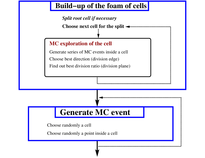
As already mentioned, the execution of the Foam algorithm is clearly separated into the first stage of the “distribution exploration” consisting of the “build-up of the foam of cells”, which in a sense memorizes the $n$-dimensional shape of the distribution, and the second stage of the actual “MC generation”, see Fig. 1. The most essential part of the present Foam algorithm is the procedure of the binary split of the cell, in which it is decided which cell is picked up for the next split and the necessary parameters of the geometry of the cell split are determined. This part of the Foam algorithm description is delegated to the next section. In the present section we describe other, more general, aspects of the Foam algorithm.

2.1 Cellular exploration of the distribution

The most obvious method to minimize the variance or maximum weight of the target weight distribution in the MC generation, already considered some 40 years ago, is to split the integration domain into many cells, so that the distribution $\rho(\vec{x})$ is approximated by $\rho^{\prime}(\vec{x})$, which is constant within each cell. This is a cellular class of the general-purpose MC algorithms.

The immediate questions are: What kind or shapes of the cells to use and how to cover the integration domain with cells? The reader may find in Ref. [6] an example of a rather general discussion of these questions. In the Foam program the user may opt for one of the three geometries of the cells: (1) simplices, (2) hyperrectangles and (3) Cartesian products of simplices and hyperrectangles. For these particular types of cells there exists an efficient method of parametrizing them in the computer memory and handling their geometry.

The system of many cells can be created and reorganized all at once, as in VEGAS-type programs [3, 4, 5], or in a more evolutionary way, as the cell split process of this work. In the Foam algorithm we rely on the binary split of cells. Starting from the entire integration domain (unit hyperrectangle or simplex) cells are split into two daughter cells, step by step, until the user-defined memory limit is reached. The choice of next cell to be split and the geometry of the split in the exploration phase are driven by the “target weight distribution” of the generation process, see Section 3. The important advantage of any cell split algorithm is that it assures automatically the full coverage of the integration domain – simply because the primary root cell is identical to the entire integration domain and the two daughter cells always cover the parent cell entirely. The problem of blind spots discussed in Ref. [6] is avoided by construction.

In the early version of Foam [1], there was a possibility in the algorithm that the “unsuccessful” branch in the tree of all cells can be erased and rebuild. This was called “collapse” and “rebuild”. In the present version this option was removed, because the experience with many testing functions has shown that the algorithm of the cell build-up is rather “deterministic” and the “rebuild” procedure was usually leading to a new branch of foam with about the same features as the old one.

Let us finally remark that the version of the cellular algorithm presented in this paper is, in fact, result of many experiments with different variants of the cellular algorithm. The presented version is the best one out of several development versions. In the code one may still see some “hooks” and unused features (class members or methods) related to these alternative variants. We have left them just in the case that some new idea of improving the algorithm emerges, or for certain kinds of debugging/testing.

2.2 Variance reduction versus maximum weight reduction

In the construction of the Foam algorithm, most effort was invested into a minimization of the ratio of the maximum weight to the average weight $w_{\max}/\langle w\rangle$. This parameter is essential, if we want to transform variable-weight events into $w=1$ events, at the latter stage of the MC generation.

Minimizing the maximum weight $w_{\max}$ is not the same as minimizing the variance $\sigma=\sqrt{\langle w^{2}\rangle-\langle w\rangle^{2}}$. Minimizing $w_{\max}$ may be more difficult – but it is worth an effort because Foam is really meant to be a part of a bigger MC program, where it is usually essential that the “inner part” of the program provides events with an excellent weight distribution, or even $w=1$ events. Nevertheless, minimizing the variance is also implemented in Foam and available optionally. It can be useful if one is satisfied with the variable-weight events, and/or if the main aim is the evaluation of the integral and not the MC simulation.

Figure 2: Weight distribution of the Foam for the default option with the maximum weight optimization (a-c) compared to analogous distributions obtained for an option with the variance optimization (d-f). Number of cells is 200, 2000 and 20000 for (a-c) and (d-f), correspondingly.

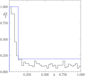
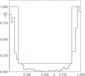
The difference between the above two options is well illustrated in Fig. 2, which shows two examples of the evolution of the MC weight distribution due to a gradual increase of the number of cells. For the default configuration, Foam optimises the ratio $w_{\max}/\langle w\rangle$. This case is shown in plots (a–c) in Fig. 2. Here, the weight distribution features a sharper and sharper drop of the weight distribution at $w=1$, while increasing the number of cells. Also, the average weight increases gradually and the weight distribution gets narrower. The optional case of the optimization of $\sigma/\langle w\rangle$ is shown in plots (d–f) of Fig. 2. In this case the variance is decreasing with the growing numbers of cells. On the other hand, the maximum weight is noticably higher than before. All weight distributions were obtained for the same 2-dimensional testing function $\rho_{b}(x)$, used also in Section 6.

2.3 Hyperrectangles or simplices?

In Ref. [1] simplical cells have been chosen instead of simpler hyperrectangles, mainly because of the author’s “prejudice” that simplices may adapt more efficiently to complicated singularities in the distribution $\rho(x)$ spanned along subspaces, not necessarily parallel to the axes of the global reference frame. Hyperrectangles tend to remember the orientation of the parent hyperrectangle, while simplices feature, in principle, a kind of “angular mobility”, i.e. they can forget the orientation of great-grand-parents, and adapt to the orientation of the singularity in $\rho(x)$. However, an experience with tens of testing functions has shown that in many cases hyperrectangles provide the same or even better final MC efficiency than simplices, for the same number of cells. Moreover, simplices have certain additional disadvantages. At present, Foam with simplices is practically limited to rather low dimensions $n\leq 5$, because in most cases the entire integration domain is a unit hyperrectangle, which has to be divided into $n!$ simplices, where $n!$ quickly becomes a large number. This limitation is, of course, not valid, if the entire integration domain is actually a simplex of high dimensionality instead of a hyperrectangle. (Foam can be configured to start cell evolution from a simplex or Cartesian product of a simplex and a hyperrectangle.) Furthermore, geometry manipulations in the simplical case require calculation of many determinants – this slows down the program execution at higher dimensions. In addition, in the present implementation, the memory consumption in a simplical foam build-up is $\sim 16\times n$ Bytes/cell, while for hyperrectangles we have found a method that limits memory consumption to below $\sim 80$ Bytes/cell independently of $n$, see Section 2.6. We can therefore reach easily the level of $10^{6}$ hyperrectangular cells at any dimension (in practice $n\leq 16$) and about $50,000$ simplical cells, for $n\leq 5$. As we see, hyperrectangular foam seems to win on many fronts. Nevertheless, we keep simplical foam as an option, because in certain applications one will definitely encounter distributions for which it turns out to be more efficient to use simplices, in spite of all their limitations, at least for a subset of the integration variables.

2.4 Build up of the foam and data organization

The foam of cells is built-up by starting from the root cell, which is the entire integration domain, through a process of binary split of a parent cell into two daughter cells. The root cell is either a unit hypercube $0\leq x_{i}\leq 1$ (default) or a simplex $0\leq x_{1}\leq x_{2}\leq x_{3}\leq\dots\leq x_{n}\leq 1$. Also a Cartesian product of these two shapes available on option. Any cell being a product of the cell split can be also a hyperrectangle, a simplex or Cartesian product of the $k$-dimensional hyperrectangle and $n$-dimensional simplex, with the total dimensionality $k+n$. If the starting root cell is a hypercube and cells are simplical (or of mixed type) then the root cell is immediately divided into $n!$ simplical (or mixed type) cells.

Each cell is explored immediately after its creation. In the exploration of the cell, about $100$-$1000$ MC events (the user may define this number) are generated inside the cell with flat (uniform) distribution and using MC weight equal to $\rho(x)$; certain averages and certain integrals over the cell are estimated. Also, the best geometry of the binary split of the cell is established and recorded for future use. In this way, every created cell is ready for an immediate split. The determination of the best split is described in fine detail in Section 3. In the exploration the estimate of the integral $R_{I}=\int_{\omega_{I}}\rho(x)dx^{n}$ is calculated for each cell $\omega_{I}$. Far more important is another functional $R_{loss}|_{I}=\int_{\omega_{I}}\rho_{loss}(x)dx^{n}$, see Section 3 for its definition, which determines the evolution of the foam and the split of the cell. Next cell to be divided into two is a cell chosen randomly, according to a probability proportional to $R_{loss}|_{I}$ or, optionally, a cell with the largest $R_{loss}|_{I}$.

The process of cell division continues until the user-defined maximum number $N_{c}$ of cells is reached. $N_{c}$ includes, in addition to the normal cells called active cell, also all cells that were split, i.e. all parents, grand-parents and great-grand-parents inluding root cell, which we shall call inactive cells. Usually, when we refer to cells, we mean both active and inactive ones. Keeping inactive cells in the record may look like a waste of the memory, but owing to the binary character of the cell split, the loss is only a mere factor of 2. There are many reasons, which make it profitable to keep all inactive cells (including the root cell) in the memory; in particular, as we shall see in Section 2.6, keeping all cells in the record will help us encode all cells in the memory in an economic way, that at higher dimensions we finally gain in terms of total consumption of the CPU memory. Furthermore, for certain quantities that are the integrals over the cell, such as $R_{I}$, we do the following: just after the split, when a new, more precise value of $R_{I}$ is known for the daughter cells – the value of the $R_{I}$ of the parent cell is updated with the sum of the contributions from two daughter cells. This correcting procedure is repeated for all ancestor cells up to the root cell. In this way, the root cell (and any other inactive cell) always keeps track of the actual value of the total $R_{I}$ during the whole foam build-up process. This can be done for any other integral quantity as well, and can be exploited for various purposes.

Since the maximum number of cells $N_{c}$ is defined at the beginning of the foam build-up, all the cell objects and/or other related objects (vertices) are allocated in the computer memory at once, at the very beginning of the cell build-up. On the other hand, the cell objects are organized as a multiply-linked list, with pointers towards parents and daughters. In addition, an array of pointers to all active cells is created at the end of the foam build-up, in order to speed-up the MC generation.

Let us now briefly explain how the geometry of an individual cell is parametrized and stored in the memory. It is relatively easy to parametrize an $n$-dimensional hyperrectangle or simplex in a way that does not require much computer memory. An $n$-dimensional simplex is fully determined by its $n+1$ vertices. Since most of the vertices are shared by the adjacent simplices, the most efficient method is to build an array of all vertices $\vec{V}_{K},K=1,2,...,N_{V}$, each of them being an $n$-component vector, and to define every simplex as a list of $n+1$ vertex indices (integers or pointers) $K_{1},K_{2},...,K_{n+1}$. For $N_{c}$ simplical cells resulting from the binary split of a single “root” simplex cell, the number of vertices is $n+1+N_{c}$, because each binary split adds one new vertex. (We include in $N_{c}$ also cells that have got split). The interior points of the simplex are parametrized as follows

$$\vec{x}=\sum_{i\neq p}^{n}\lambda_{i}(\vec{V}_{K_{i}}-\vec{V}_{K_{p}}),\quad\lambda_{i}>0,\quad\sum_{i\neq p}\lambda_{i}<1,\quad i=1,2,\dots,n,$$ (1)

using basis vectors relative to the $p$-th vertex. The above method would be inefficient for $n$-dimensional hyperrectangles, because memorizing all $2^{n}$ vertices would require too much memory at higher dimensions. Instead, we use another way of parametrization: each hyperrectangle is defined by the $n$-dimensional vector $\vec{q}$ defining the origin of the cell and another vector $\vec{h}=(h_{1},h_{2},...,h_{n})$, where each component $h_{i}$ is the length of the hyperrectangle along the $i$-th direction. This is even clearer from the explicit parametrization of the interior of the hyperrectangle:

$$x_{i}=q_{i}+\lambda_{i}h_{i},\quad 0<\lambda_{i}<1,\quad i=1,2,\dots,k.$$ (2)

For cells with mixed topology, we apply Eq. (2) for $i=1,2,\dots,k$ and Eq. (1) for $i=k+1,k+2,\dots,k+n$. In Section 2.6 we describe an optional method of storing hyperrectangular cells, in which just two integer numbers are recorded instead of two vectors $\vec{q}$ and $\vec{h}$ (two 2-Byte integers instead of $2n$ of 8-Byte floating-point numbers). This method is implemented for the hyperrectangular part of the space only.

2.5 Monte Carlo generation

Once the build-up of the cells is finished, the Monte Carlo generation takes place. There is no need for any reorganization of the cells. MC generation can be started immediately. The only thing, that is done at the very end of the foam build-up is the preparation of the list of pointers to all active cells and the array of corresponding $R^{\prime}_{I}$.

The MC point is generated in two steps. First, a cell is chosen with a probability proportional to $R^{\prime}_{I}=\int_{x\in Cell_{I}}\rho^{\prime}(x)$ and next a MC point $x$ is chosen with uniform probability inside the cell. The MC weight $w=\rho^{\prime}(x)/\rho(x)$ is associated with the event. For a successful foam of cells, the MC weight is close to 1 and the user may turn weighted events into $w=1$ event by means of the rejection method (with the acceptance rate $\sim\langle w\rangle/w_{\max}$). Foam can do this also for the user. However, the user can sometimes organize the calculation of the $\langle w\rangle$ and bookkeeping of other parameters of the weight better, in a way that best fits his own aims. This is why the mode of variable weights MC events is also available. The total integral, usually necessary for the proper normalization of the MC sample, is calculated using $R=R^{\prime}\langle w\rangle$. Foam program provides both the exact value of the $R^{\prime}$ and the MC estimate of the integral $R$.

2.6 Economic use of the computer memory

The actual implementation of the single cell object occupies about 80 Bytes (it could be shrinked to about 40 Bytes, if necessary) of various integer and double precision attributes, plus the dimension-dependent part. In the case of a simplical cell, each new cell adds one $n$-component double-precision vector (vertex) and the total memory consumption is therefore of order $(80+8\times n)$ Bytes/cell. For $n=5$ and 100K cells it is therefore $\sim$ 15 MBytes of the memory, still an affordable amount. For the hyperrectangle cells we have to count two $n$-component double-precision vectors per cell, that is about $(80+16\times n)$ Bytes/cell. For the $10^{6}$ cells and $n=15$ that would mean $\sim$ 340 MBytes for the entire foam of cells, which could be annoying. Fortunately, we have found a method of substantially reducing the memory consumption for a hyperrectangular foam. As discussed in Section 3 the geometry of the cell division is fully determined in terms of two integers: one of them is the index of an edge to which the division plane is perpendicular and the other one defines the position of a division plane. The position parameter is a rational number, and only the integer numerator has to be remembered, while the denominator is common to all cells. The above two integers define uniquely the position of the two daughter cells relative to a parent cell. With this method the memory consumption is down to about 80 Bytes/cell, independently of $n$ in the present implementation. There is, however, a price to be payed in terms of CPU time. For the generation of the point inside a cell, or even the evaluation of the weight, we need the “absolute” components of $x$, that is in the reference frame of the root cell, not relative to vertices of the cell. It is therefore necessary to use a procedure (a method in the class of cells) to construct the absolute position of a given cell “in flight”. This is done by means of tracing all ancestors of a given cell up to the root cell and translating position and size with respect to its parent into absolute ones, step by step, finally relative to the root cell. It is implemented exploiting the organization of cell objects into a linked binary tree. The average number of ancestor cells to be traced back from a given active cell up to the root cell for $N_{c}=10^{6}$ cells is on the average about $\ln_{2}N_{c}\sim 20$. This may cause about $20\%$ increase in the CPU time of the MC generation – an affordable price, if we remember that the MC efficiency improves mainly with the increase of $N_{c}$. In principle, this kind of memory-saving arrangement is also possible for simplical cells; however, in this case the CPU time overhead would be larger, because of the necessity of the full linear transformation at each step, on the way from a given cell up to the root cell. In the case of hyperrectangular cells the transformation is much simpler (and faster); it is the translation and/or dilatation along a single spatial direction at each step.

Figure 3: Inhibited cell division for first variable, that is for $x_{1}$ (right). Foam with 250 cells.

2.7 CPU time saving solution

The final MC efficiency is improved mainly by increasing the number of cells $N_{c}$. The CPU time of the cell build-up is $T\sim n\times N_{c}\times N_{samp}$, where $N_{samp}$ is the number of MC events used in the exploration of each newly created cell. The important practical question is: Can one somehow reduce $N_{samp}$ without much loss of final MC efficiency, in order to be able to increase $N_{c}$, within the same CPU time budget?

A simple solution is the following: during the MC exploration of a new cell we continuously monitor an accumulated “number of effective events with $w=1$” defined [7] as $N_{eff}=(\sum w_{i})^{2}/\sum w_{i}^{2}$, and terminate cell exploration when $N_{eff}/n_{bin}>25$, where $n_{bin}$ is the number of bins in each histogram, which is used to estimate the best division direction/edge parameters. This method helps to cut on the total CPU time, because the increase of $N_{samp}$ is not wasted for cells in which the distribution $\rho(x)$ is already varying very little. At the later stage of the foam evolution this happens quite often. In this method the user may set $N_{samp}$ to a very high value and the program will distribute the total CPU time (in terms of $N_{samp}$) among all cells economically, giving more CPU time to those cells really need it, i.e. to cells with the stronger variation of $\rho(x)$.

2.8 Inhibited variables – flat dependence

In some cases the user may not want Foam to intervene into certain variables in the distribution $\rho(x)$, simply because there is little or no dependence on them in $\rho(x)$. The user may draw, of course, these variables directly from any uniform random number generator. He may, however, find it more convenient to get them from the Foam program. This is easily implemented in Foam: any variable $x_{i}$ may be “inhibited” for the purpose of cell-splitting procedure. In the Foam code it is actually done in such a way that Foam excludes this variable (edge) from the procedure of determining the best binary division of the cell. This provision makes practical sense mainly for the hyperrectangular part of the variable subspace.

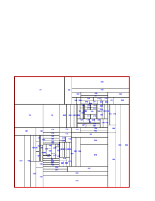
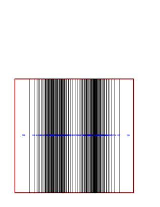
In Fig. 3 we show two 2-dimensional foams (250 cells) for the same testing distribution $\rho(x)$ (two Gaussian peaks on the diagonal). In one of them (right plot) we have inhibited a split in the first variable, that is for $x_{1}$.

Figure 4: Predefined division points at $x_{1}=0.30,0.40,$ and $0.65$, for 2000 cells.

2.9 Predefined split points – provision for very narrow peaks

In the practical applications, see Refs. [17, 18], one may encounter in certain variables extremely narrow spikes (narrow resonances). The Foam exploration algorithm may find it difficult to locate these spikes with the usual method of MC sampling in the cells, at the early stage of the foam build-up. For very narrow spikes, or too low number of requested cells, it may not find them at all! The user usually knows in advance the position of these spikes and the Foam should have a built-in mechanism to exploit this knowledge.

The solution is simple. (It applies for the hyperrectangular subspace of the parameter space only.) The user has a possibility to provide Foam, for each variable, with the list of a number of predefined values: the first splitting positions of the root cell. In the Foam algorithm, it is checked if the list of predefined division points is not empty. If it is the case, then instead of adopting the division parameter from the usual procedure described in Section 3, Foam takes the division parameter from the list, and removes it from the list. In this way the first few division points are taken from the “user-defined menu”, if available, and the next ones are chosen with the usual methods. For narrow spikes this method helps Foam to locate and surround them with as a dense group of cells as necessary.

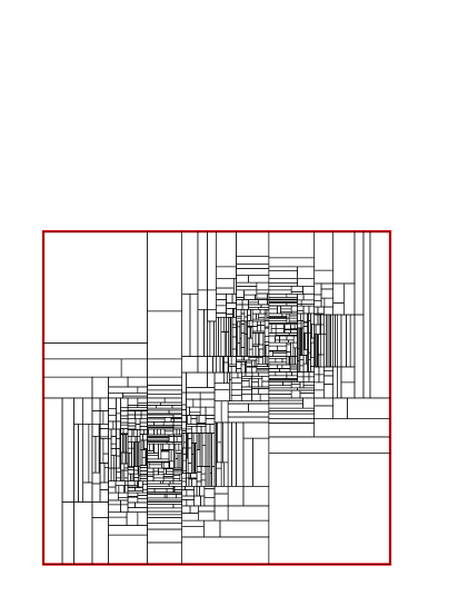
In Fig. 4 we show an example with two Gaussian peaks in which we requested the Foam program to use the three predefined division points for the $x_{1}$ variable. They are clearly seen as three vertical division lines dividing the entire root cell. In the present case, peaks are not so narrow and there is no real need for a predefined division. The example is just to illustrate the principle of the method.

2.10 Mapping of variables

If the structure of the singularities is known and/or Foam is unable to get a reasonable weight distribution for a reasonable number of cells, it is then worth performing an additional change of variables, so that the transformation Jacobian compensates for the singularities, at least partly. In such a case the user subprogram provides Foam with the distribution

$$\rho^{\star}(y)=\frac{d\rho}{dy_{1}\dots dy_{n}}=\rho(x_{1}(y),x_{2}(y),\dots,_{n}(y))\left|\frac{\partial x^{(j)}(y)}{\partial y}\right|,$$ (3)

instead of the original $\rho(x)=d^{n}\rho/dx^{n}$. For each vector $y$ generated by Foam, the image vector $x$ is well known in the subprogram calculating $\rho^{\star}(y)$. A mechanism for exporting $x$ to the outside world usually has to be provided by the user, because Foam cannot help – it does not know anything about $x$; it only knows $y$.

Note that in the limiting case of the “ideal mapping” we have

$$\left|\frac{\partial x(y)}{\partial y}\right|\equiv\frac{R}{\rho(x)};$$ (4)

consequently, $\rho^{\star}(y)=R$ and in this case Foam would play merely the role of a provider of the random numbers for $y$.

The user of Foam may also need to apply mapping in the case of a “weak” integrable singularity in the distribution $\rho$ like $\log(x)$ or $\sqrt{x}$. Foam can deal with them by brute force, at the expense of a larger number of cells. However, a wiser approach is to apply mapping, in order to remove such singularities from the distribution.

In the next section we shall describe how to combine the mapping method with the multibranching. Such a mixture is well known as the most powerful method of improving the efficiency of the Monte Carlo method.

2.11 Provisions for the multibranching

In the following we elaborate on the various methods of implementing multibranching MC method [19, 20, 21, 22] with the help of Foam.

2.11.1 Single discrete variable

As a warm-up exercise, let us consider the question: Is Foam capable to generate (and sum up) a discrete variable $i=1,2,\dots,N,$ according to the (unnormalized) distribution $r_{1},\dots,r_{N}$? Of course it can. The simplest way is to define an auxiliary 1-dimensional distribution

$$\rho(x)=r_{i},\quad\hbox{for}\;\;\frac{i-1}{N}\leq x\leq\frac{i}{N},\;\;i=1,2,\dots,N.$$ (5)

The user subprogram providing the above $\rho(x)$ is trivial. If plotted, this $\rho(x)$ would look like a histogram with $N$ equal-width bins. Foam will build up its own grid of cells (intervals), and if we request a high enough number of cells (that is $N_{c}>N$), it will approximate the above $\rho(x)$ very well, with its own “histogram-like” distribution $\rho^{\prime}(x)$. However, the Foam approximation will never be ideal, because Foam is not able to detect the exact position of the discontinuities in $\rho(x)$. (Nevertheless, this will be a workable solution with a very good weight distribution.) The present Foam algorithm provides for an essential improvement: one may predefine the division points as $x^{(i)}=i/N$, $i=1,\dots,N$, and set the number of cells to be $N_{c}\geq N$. In such a case Foam will define its cells matching exactly the shape of $\rho(x)$. It will generate points with $w\equiv 1$ and provide the exact sum $R=R^{\prime}=\sum r_{i}$, already at the end of the foam build-up. In the MC generation, Foam will randomly generate variable $x\in(0,1)$, which can be translated easily into discrete $i$ $1\leq i\leq N$.

2.11.2 Discrete and continuous variables

How does the above extend to the case of the distribution $\rho$ depending on one discrete variable and the usual $n$ continuous variables? For such a distribution $\rho(y_{1},\dots,y_{n},i)$ we define

$$\rho(x_{1},x_{2},\dots,x_{n+1})=\rho(x_{1},\dots,x_{n},i),\quad\hbox{for}\;\frac{i-1}{N}\leq x_{n+1}\leq\frac{i}{N},\;\;i=1,2,\dots,N,$$ (6)

in completely analogy with Eq. (5). As previously, we provide for the variable $x_{n+1}$ a list of predefined division points $x_{n+1}^{(i)}=i/N,\;i=1,2,\dots,N$, and, of course, we request $N_{c}>>N$. There is still one small problem: Foam may “by mistake” perform an unnecessary cell division for the variable $x_{n+1}$, simply due to statistical errors in the “projection histogram” described in Section 3.4.1. This problem is solved in Foam in an elegant way: in addition to providing for $x_{n+1}$ predefined division points, the user of Foam may declare $x_{n+1}$ as an “inhibited variable” in the sense of Section 2.8. In this case Foam will still split cells according to a list of predefined division points for $x_{n+1}$, but will not perform any additional division in this variable! (The translation of the continuous $x_{n+1}$ to the discrete $i$ is done as usual.) The above method is the basic method of implementation of the “multibranching” (or “multichannel”) MC method using Foam. Let us call it “predefined and inhibited division”, for short PAID method. We shall also describe below how to combine the PAID method with mapping, etc.

In order to appreciate more fully the advantages of PAID, let us consider a more straightforward implementation of the multibranching. In the object-oriented environment one may easily construct $N$ instances of the Foam object, each of them for the $n$-dimensional function $\rho(x_{1},\dots,x_{n},i)$, initialize them (creating a separate foam of cells) and generate event $(x,i)$ with the associated weight $w_{i}(x)$. Index $i$ can be chosen according to probability $p_{i}=R^{\prime}_{i}/\sum_{j}R^{\prime}_{j}$, where $R^{\prime}_{i}$ are provided by the $i$-th object of the Foam class (at the end of its initialization). The total weight of the event is $w(x,i)=w_{i}(x)/p_{i}$. Let us call this scenario an “externally organized multibranching”, for short EOM.

Both methods have certain advantages and disadvantages. In PAID the user does not need to organize the optimal/efficient generation of the branching index $i$. The root cell is divided into $N$ equal-size sub-root cells, which then evolve separately into an independent system of cells, adapting individually to the singularities in the $i$-th component of $\rho$. Foam adjusts the relative importance of the sub-root cells and their descendants, and finds automatically the optimal number of the division cells in the $N$ subfoams within the requested total memory limit. In the EOM scheme these adjustments for the individual branches has to be done by the user. On the other hand, in some cases, the user may want to configure the Foam objects for each branch individually. In the EOM scheme, this can be done for each Foam object separately. In the PAID scheme this cannot be done, because all cells have the same properties, the cell-split algorithm is the same, the cell geometry is common, etc. In most cases, the PAID method will be preferred, because it is easier to organize.

In the following we shall concentrate on the PAID scheme. In this case, the normalization integral is provided by the Foam at the end of the exploration phase, and it includes the sum over a discrete variable:

$$R^{\prime}=\sum_{i=1}^{N}\int\rho_{i}^{\prime}(x)dx^{n}.$$ (7)

We also have the usual relation between the average weight and the integral

$$R=\sum_{i=1}^{N}\int\rho(x)_{i}dx^{n}=R^{\prime}\;\langle w\rangle.$$ (8)

The above method extends trivially to the case of several discrete variables. As already stressed, the relative probabilities of the discrete components $p_{i}\sim R^{\prime}_{i}=\int\rho^{\prime}_{i}(x)dx^{n}$ in the MC generation are automatically adjusted by the Foam algorithm, so that the maximum weight or the total invariance is minimized. In the EOM scheme, arranging this in the user program would require an extra programming effort, while in the PAID method this comes for free, by exploiting standard Foam functionality.

2.11.3 Multilayer method

There is an alternative PAID-type method of dealing with the problem of the discrete variable, which generates points according to $\rho(x_{1},\dots,x_{n},i),\;i=1,2,\dots,N$. It will produce the same distribution but will differ from PAID in the MC efficiency, in terms of the maximum weight or variance. One may simply generate, with the help of Foam, the $n$-dimensional auxiliary distribution

$$\bar{\rho}(x_{1},\dots,x_{n})=\sum_{j=1}^{N}\rho(x_{1},\dots,x_{n},j)$$ (9)

and next, for each generated $x$, choose randomly a discrete variable $i$ according to the probability

$$p_{i}(x)=\rho(x,i)/\sum_{j=1}^{n}\rho(x,j).$$ (10)

Let us call it PAID^∗, or the multilayer method. This method is slightly less convenient to implement, as is clearly seen for $n=0$, where the user effectively has to generate by himself the discrete variable $i=1,2,\dots,N$ according to the above probability, by means of creating an inverse cumulative distribution, mapping a random number into $i$, etc., while in the standard PAID scenario all this job is done by the Foam program. Furthermore, in the PAID method each component distribution $\rho(x,j)$ may have a “cleaner” structure of the singularities than the sum. Consequently, in the PAID method Foam will probably find it easier to learn the shape of each component distribution than that of the sum in PAID^∗. These two kinds of equivalent multibranching algorithms, PAID and PAID^∗, are described and analysed in Ref. [21]. The PAID^∗ method is used in the KKMC event generator of Ref. [18] to generate index $i$ numbering the type (flavour) of the produced quark or lepton.

2.11.4 Multibranching and mapping

However, the most important reason for setting up Foam according to the PAID scenario, with the separate foam build-up for each component distributions $\rho(x,j)$, is that for each component one may apply individually adjusted mapping of variables, which makes every component distribution much less singular. The combination of the mapping and multibranching is probably the most powerful known methods of improving MC efficiency [20, 21]. How it can be actually realized with the help of Foam depends on the properties of the distribution $\rho(x)$ to be generated. In the case where we have an explicit sum over many components

$$\rho(x_{1},\dots,x_{n})=\sum_{j=1}^{N}\rho(x_{1},\dots,x_{n},j),$$ (11)

each of the components being positive, with a distinctly different and well known structure of the singularities, we would recommend the use of Foam in the PAID scheme. Knowing the structure of singularities, we may be able to introduce mapping in each component separately, which compensates for these singularities with the Jacobian factor. In such a case Foam is provided with the following distribution:

$$\rho(y_{1},\dots,y_{n},j)=\rho(x^{(j)}_{1}(y),\dots,x^{(j)}_{n}(y),j)\;\left|\frac{\partial x^{(j)}(y)}{\partial y}\right|,\;\;j=1,2,\dots,N,$$ (12)

understanding that the translation of the discrete index $j$ into a continuous variable $y_{n+1}$, is done in the usual way. The foam of cells is, of course, build-up in the $y$-variables, different for each $j$-th branch. The user is fully responsible for the proper mapping $x^{(j)}(y),\;j=1,2,\dots,N$, and the calculation of the Jacobian factor in every component (branch). In the user subprogram providing the $\rho$-distribution, the variable $y_{n+1}$ will first be translated into index $j$ and then, depending on the value of $j$, a given type of mapping will be applied. For the outside part of the code, the index $j$ can be made available, or it may be hidden (erased from the record), depending on the needs of a specific application.

In some cases, however, one does not know any unique way of splitting the $\rho(x)$ into well defined positive components as Eq. (12), but one may have a rough idea about the leading singularities. This means, that one is able to construct the distribution

$$\rho(x_{1},\dots,x_{n})\sim\bar{\rho}(x_{1},\dots,x_{n})=\sum_{j=1}^{N}\bar{\rho}(x_{1},\dots,x_{n},j),$$ (13)

where $\bar{\rho}(x,j)$ have the same type of the leading singularities as $\rho(x)$, and one controls the normalization of singularities in $\rho(x)$ up to a constant factor; that is for $x$ in the neighbourhood of the $j$-th singular point, a line or a (hyper)plane, only $\bar{\rho}(x,j)$ really matters, that is $\rho(x)\simeq C_{j}\bar{\rho}(x,j)$, where $C_{j}$ is not known a priori.

In addition, let us assume that we are able to compensate for the singularities in each $\bar{\rho}(x,j)$ exactly by dedicated mapping specific to singularities in the $j$-th branch. In other words, the mapping is ideal in each branch:

$$\left|\frac{\partial x^{(j)}(y)}{\partial y}\right|=\frac{\bar{R}_{j}}{\bar{\rho}(x,j)}.$$ (14)

The above also means, that we know analytically the exact values of the integrals: $\bar{R}_{j}=\int\bar{\rho}(x,j)dx^{n}$.

In such a case we may employ the algorithm of Foam successfully by means of defining the “branching ratio”

$$b_{j}(y_{1},\dots,y_{n})=\bar{\rho}(y_{1},\dots,y_{n},j)/\bar{\rho}(y_{1},\dots,y_{n}),\quad\sum b_{i}(y)=1,$$ (15)

constructing the distribution to be digested by Foam as

$$\rho(y_{1},\dots,y_{n},j)=b_{j}(x)\rho(x^{(j)}_{1}(y),\dots,x^{(j)}_{n}(y))\;\left|\frac{\partial x^{(j)}(y)}{\partial y}\right|=\frac{\bar{R}_{j}\;\rho\big{(}x(y)\big{)}}{\sum_{l}\bar{\rho}\big{(}x(y),l\big{)}},$$ (16)

and proceeding as in the PAID scheme described previously.

The role of the function $b_{j}(x)$ is to isolate out from $\rho(x)$ “a layer” including just one known type of singularity. In order to see how this method works, let us consider a $\delta^{(n)}(x-a)$ shape singularity in the $j$-th component (narrow Gaussian peak etc.) of size $\epsilon$. Then, in the vicinity of that singularity we have $b_{j}(x)=1$ and $\rho(x)\simeq C_{j}\bar{\rho}(x,j)$, while further away we have $\rho(x)\sim{\cal O}(\epsilon^{n})$. The Foam program will, of course, include the $C_{j}$ factor properly in the normalization, and build up the foam of cells everywhere, close to a singularity and far away. It will do it really not in the $x$ variables but in the $y$ variables. Now, the mapping $x\to y$ (specific to the $j$-th branch) will expand the singularity neighbourhood of ${\cal O}(\epsilon)$ into a region of size of ${\cal O}(1)$, while the $y$-image of the remaining $x$-space will be of the size ${\cal O}(\epsilon)$. This can be the source of the following drawback: in the small $y$-domain of ${\cal O}(\epsilon)$ described above, at the positions of the singularities from the other components $i\neq j$, $\rho(y,j)$ may get narrow spikes or dips of height of ${\cal O}(1)$, such that their integral contribution will be negligible, of ${\cal O}(\epsilon^{n})$, and this may not look as a problem. However, the Foam algorithm may find it difficult to locate these structures, and this may lead to a small but finite bias of the generated distributions and calculated integrals. This should be kept in mind, and special tests (MC runs with a maximum number of cells, and high MC statistics) should be performed, in order to check that this effect is absent.

The above method is quite similar to that of Ref. [20]. One difference is that in the latter there are several iterations with an aim af adjusting the relative normalization of the components $\bar{\rho}(x_{1},\dots,x_{n},j)$ to $\rho(x)$. Our scheme could effectively be regarded as the method of Ref. [20] with just one iteration; that is the first step being the foam build-up, and the second step (1st iteration) being the MC simulation. One iteration is sufficient in the limit of vanishing overlap of the components $\bar{\rho}(x_{1},\dots,x_{n},j)$ in the entire $\bar{\rho}(x)$. While in the method of Ref. [20] a better adjustment is provided by the next iterations, in Foam the cellular adaptive method provides an extra mileage. One cannot therefore say which one is better in general – it depends on the distribution $\rho(x)$.

In fact, in the PAID scheme with the mapping, extra iterations are also possible. It can be done as follows: (a) read $R_{j}$ from all $N$ “leading cells” after the foam build-up, (b) rescale $\bar{\rho}(y_{1},\dots,y_{n},j)\to(R_{j}/\bar{R}_{j})\bar{\rho}(y_{1},\dots,y_{n},j)$, and (c) repeat the foam build-up for the new branching ratios $b_{j}(x)$ in Eq. (16). The above procedure can be repeated. Whether such an iteration is profitable depends on the particular distribution – we expect that in most cases it is not necessary, thanks to the adaptive capabilities of Foam.

Last, but not least, let us also consider the case of a sum of integrals with different dimensionality or, in other words, the distribution in which the number $n_{i}$ of the continuous variables $x_{1},...,x_{n_{i}}$ depends on a certain discrete “master variable” $i=1,...,N$ (for example $n_{i}=i$):

$$R=\sum_{i=1}^{N}\int\rho_{i}(x_{1},...,x_{n_{i}}).$$ (17)

Foam can deal with this case too. The simplest solution is to find the maximum dimension $n_{\max}$ and add extra dummy variables on which some of $\rho_{i}$ does not depend, such that formally all sub-distributions have the same dimension $n_{\max}$. In this way one is back to a situation described earlier, and may apply the PAID method, with or without the additional mapping. The slight drawback of this solution is that in the present implementation of Foam we cannot inhibit the unnecessary cell divisions across the directions of the newly introduced dummy variables – simply because they are not the same in all branches. This is the reason why this kind of problem can, in some cases, be dealt with more efficiently using the EOM scenario, with a separate Foam object for each branch.

For additional practical examples on how to realize multibranching with Foam, see Section 6.

3 Cell split algorithm and geometry

As already indicated, our algorithm of the cell split covers two strategies: (A) minimization of the maximum weight $w_{\max}$ and (B) minimization of the variance $\sigma$, where both $w_{\max}$ and $\sigma$ are calculated in the Monte Carlo generation, using the MC weight $w=\rho/\rho^{\prime}$. The distribution $\rho^{\prime}$ is the result of the exploration (it is constant over each cell) and is frozen at the end of exploration. The subsequent MC event generation of events is done according to $\rho^{\prime}(x)$. Its integral $R^{\prime}=\int\rho^{\prime}(x)d^{n}x$ has to be known exactly before the start of the MC generation. On the other hand, the best estimate of the integral $R=\int\rho(x)d^{n}x$ is obtained, up to a statistical error, at the end of the MC event generation with the usual relation: $R=R^{\prime}\langle w\rangle_{\rho^{\prime}}$. The average $\langle...\rangle_{\rho^{\prime}}$ is over events generated according to $\rho^{\prime}$.

There is another important ingredient in the algorithm of the cell split: in addition to the auxiliary distributions $\rho^{\prime}(x)$ we also define another distribution $\rho_{loss}(x)$ related to the integrand $\rho(x)$. The important role of the distribution $\rho_{loss}(x)$ is to guide the build-up of the foam of cells; the function $R_{loss}=\int\rho_{loss}d^{n}x$ is minimized in the process – its value is decreasing step by step, at each cell split. Obviously, both $\rho_{loss}(x)$ and $\rho^{\prime}(x)$ are evolving step by step during the foam build-up. Once the division process is finished, the distribution $\rho_{loss}(x)$ is not used anymore; MC events are generated with $\rho^{\prime}(x)$. Nevertheless, $\rho_{loss}(x)$ is strongly related to the properties of the weight distribution in the MC generation phase.

(A) In the case when our ultimate aim is to minimize $w_{\max}$, we define

$$\begin{split}&\rho^{\prime}(x)\equiv\max_{y\in Cell_{I}}\rho(y),\quad\hbox{for}\quad x\in Cell_{I},\\ &R_{loss}=\int d^{n}x\;[\rho^{\prime}(x)-\rho(x)]=\int d^{n}x\;\rho_{loss}(x).\end{split}$$ (18)

The distribution $\rho_{loss}$ is the difference between the “ceiling distribution” $\rho^{\prime}$ and the actual distribution $\rho$ from which it is derived. The rejection rate in the final MC run is just proportional to the integral over the loss distribution $\rho_{loss}(x)$ by construction, i.e. the rejection rate $=R_{loss}/R$. (This justifies the name “loss”.) The distribution $\rho_{loss}(x)$ also has a clear geometrical meaning, see below.

(B) In the case when we do not care so much about the maximum weight and the rejection rate, but we want rather to minimize the ratio of the variance to the average of the weight, $\sigma/\langle w\rangle$, in the final MC generation, we are led to the following definition:

$$\begin{split}&\rho^{\prime}(x)\equiv\sqrt{\langle\rho^{2}\rangle_{I}},\quad\hbox{for}\quad x\in Cell_{I},\\ &\rho_{loss}(x)\equiv\sqrt{\langle\rho^{2}\rangle_{I}}-\langle\rho\rangle_{I},\quad\hbox{for}\quad x\in Cell_{I}.\end{split}$$ (19)

The average $\langle...\rangle_{I}$ is over the $I$-th cell; see Appendix A for a detailed derivation of the above prescription. The ratio $\sigma/\langle w\rangle$ in the final MC generation is a monotonous ascending function of $R_{loss}=\int\rho_{loss}(x)dx^{n}$, see Appendix A. Consequently, minimization of $R_{loss}$ is equivalent to minimization of $\sigma/\langle w\rangle$.

3.1 Rules governing the binary split of a cell

The basic rules governing the development of the foam of cells are the following:

• For the next cell to be split we chose a cell with the largest $R_{loss}$.

• The position/direction of a plane dividing a parent cell into two daughter cells $\omega\to\omega^{\prime}+\omega^{\prime\prime}$ is chosen to get the largest possible decrease $\Delta R_{loss}=R_{loss}^{\omega}-R_{loss}^{\omega^{\prime}}-R_{loss}^{\omega^{\prime\prime}}$.

How is the split of a given cell into two daughter cells in step (b) done in practice? The method relies upon a small MC exercise within a cell, in which a few hundreds of events are generated with a flat distribution. They are weighted with $\rho(x)$ and projected onto $k$ (hyperrectangular case) or $n(n+1)/2$ (simplical case) edges of the cells. In the mixed case of a cell being the Cartesian product of a $k$-dimensional hyperrectangle and an $n$-dimensional simplex, there are $k+n(n+1)/2$ projections/edges. Resulting histograms are analysed and the best “division edge” and “division hyperplane position” are found – the one for which the estimate (forecast) of the $\Delta R_{loss}$ is the largest. In the actual Foam algorithm, each new-born cell is immediately explored, its $R_{loss}$, $R$ and $R^{\prime}$ are calculated, and the best candidate as to the direction and position of the dividing plane are established and memorized, as the attributes of the cell; see below for details. In this way, every newly created cell is ready for an immediate binary division.

3.2 Geometry of the binary split of a cell

Figure 5: Geometry of the split of a 3-dimensional cell, simplex or hyperrectangle.

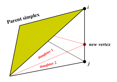
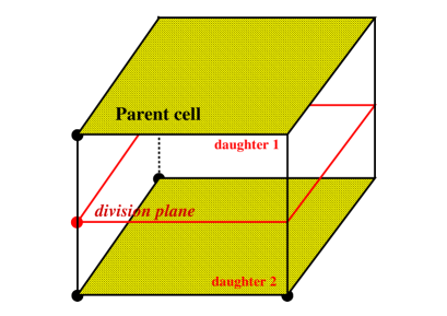
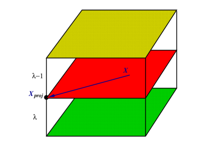
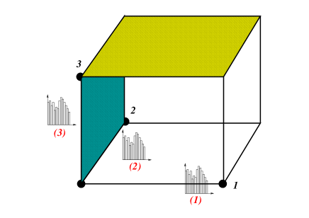
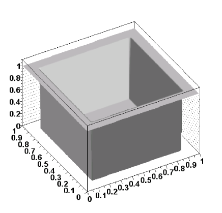
In Fig. 5 we show a 3-dimensional cell being a simplex or a hyperrectangle and we visualize the geometry of their split.

Let us first describe the split of the $n$-dimensional simplical parent cell into two daughter cells. In this case [1] we need to know which of $n(n+1)/2$ edges defined by any pair of vertices of a given simplex is the best for the split. Suppose that it is an edge defined by a pair of indices $(i,j),\;i\neq j,$ where $i,j=1,2,...,N_{V}$, of the vertices $(\vec{V}_{K_{i}},\vec{V}_{K_{j}})$, see Sect. 2.4 for the method of numbering the vertices. A new vertex $V_{N_{V}+1}$ is put somewhere on the line (edge) in between the two vertices:

$$V_{N_{V}+1}=\lambda\vec{V}_{K_{i}}+(1-\lambda_{div})\vec{V}_{K_{j}},\;\;0<\lambda_{div}<1,$$ (20)

where the division parameter $\lambda_{div}$ is determined by using an elaborate procedure described later in this section, and the number of vertices is updated $N_{V}\to N_{V}+1$. With the new vertex two daughter simplices are formed with the following two lists of vertices (their pointers):

$$\begin{split}(K_{1},K_{2},...,K_{i-1},(N_{V}+1),K_{i+1},...,K_{j-1},K_{j},K_{j+1},...,K_{n},K_{n+1}),\\ (K_{1},K_{2},...,K_{i-1},K_{i},K_{i+1},...,K_{j-1},(N_{V}+1),K_{j+1},...,K_{n},K_{n+1}).\end{split}$$ (21)

For the $k$-dimensional hyperrectangular cell defined with a pair of vectors $(\vec{q},\vec{h})$ we first decide on the direction of the division hyperplane. Assuming that this hyperplane is perpendicular to the $i$-th direction, the two daughter cells (a) and (b) are defined with the two pairs of new vectors as follows:

$$\begin{split}&\vec{q}^{(a)}=(q_{1},q_{2},\dots,q_{k}),\quad\vec{h}^{(a)}=(h_{1},h_{2},\dots,h_{i-1},h_{i}\lambda_{div},h_{i+1},\dots,h_{k}),\\ &\vec{q}^{(b)}=(q_{1},\dots,q_{i-1},q_{i}+h_{i}\lambda_{div},h_{i+1},\dots,q_{k}),\quad\vec{h}^{(b)}=(h_{1},\dots,h_{i-1},h_{i}(1-\lambda_{div}),h_{i+1},\dots,h_{k}).\end{split}$$ (22)

The 3-dimensional case of the simplical and hyperrectangular cell split made in this way is illustrated in Fig. 5.

Figure 6: Geometry of the split of the 3-dimensional simplex cell.

Figure 7: Geometry of the split of the 3-dimensional hyperrectangular cell.

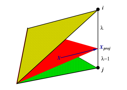
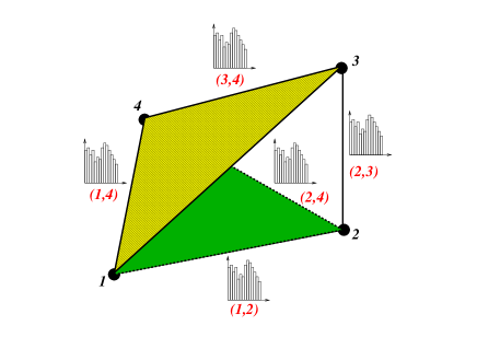
3.3 Projecting points into an edge

Before we describe the determination of the division edge and of the division parameter $\lambda_{div}$, let us still discuss certain geometric aspects of the Foam algorithm – that is how we project a point $\vec{x}$ inside a cell onto one of the edges of the cell. In the case of a simplex the edges are numbered by the pair of indices $(i,j)$, $i>j$, which number edges spanned by a pair of vertices $(\vec{V}_{K_{i}},\vec{V}_{K_{j}})$, while in the case of the hyperrectangle the $i$-th edge is spanned by the pair of vectors $\vec{q}$ and $\vec{q}_{+}=(q_{1},\dots,q_{i-1},q_{i}+h_{i},\dots,q_{n})$. The point $x$ inside a cell is projected onto the edge and parametrized using the parameter $\lambda\in(0,1)$. The parameter $\lambda$ will be used to define an auxiliary projection $d\rho/d\lambda$ for each edge in the following subsection. In particular we have to know how to evaluate $\lambda$ in an efficient way. In the case of a simplex cell we have:

$$\vec{x}_{proj}=\lambda\vec{V}_{K_{i}}+(1-\lambda_{ij})\vec{V}_{K_{j}},\;\;0<\lambda_{ij}<1,$$ (23)

where

$$\begin{split}&\lambda_{ij}(\vec{x})=\frac{|{\rm Det}_{i}|}{|{\rm Det}_{i}|+|{\rm Det}_{j}|},\\ &{\rm Det}_{i}={\rm Det}(\vec{r}_{1},\dots,\vec{r}_{i-1},\vec{r}_{i+1},\dots,\vec{r}_{n},\vec{r}_{n+1}),\\ &{\rm Det}_{j}={\rm Det}(\vec{r}_{1},\dots,\vec{r}_{j-1},\vec{r}_{j+1},\dots,\vec{r}_{n},\vec{r}_{n+1}),\qquad\vec{r}_{j}=\vec{V}_{K_{j}}-\vec{x},\end{split}$$ (24)

and ${\rm Det}(x_{1},x_{2},...,x_{n})$ is determinant. The case of a hyperrectangular cell is much simpler:

$$\lambda_{i}=(x_{i}-q_{i})/h_{i}.$$ (25)

Obviously, owing to the time-consuming evaluation of the determinants at higher dimensions, the above projection procedure will be much slower for simplices than for hyperrectangles.

In Fig. 6 we illustrate a projection procedure into six edges for 3-dimensional simplex and in Fig. 7 the case of the three edges of the 3-dimensional hyperrectangular cell.

Figure 8: Projection histogram. The case of optimizing the maximum weight.

3.4 Determination of an optimal division edge and of $\lambda_{div}$

Our aim is to find out which division hyperplane, cutting through which edge, provides the best gain of the total integral $R_{loss}$, summed over two daughters, as compared to the parent cell. In order to do that, we first analyse all possible division planes, for all edges, and find out the best one, in terms of the gain in $R_{loss}$. In other words, we go through all edges ($k$ edges for a hyperrectangle and/or $n(n+1)/2$ for a simplex) and find, for each edge, the optimal parameter $\lambda_{div}$ and the corresponding best gain in $R_{loss}$. We then compare between the gains in $R_{loss}$ for all edges and define the optimal edge as the one with the best gain in $R_{loss}$. The procedure of finding the best $\lambda_{div}$ is essentially the same for simplical and hyperrectangular cells; on the other hand, in the algorithm for finding the best $\lambda_{div}$ there is a difference between the cases of optimization of the maximum weight and of the variance; see the following discussion.

3.4.1 Optimization of the maximum weight – choosing $\lambda_{div}$

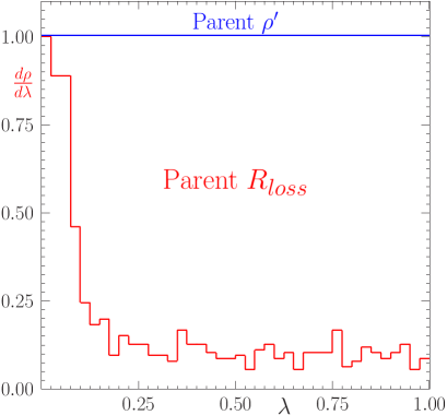
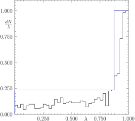
Let us consider first the case of finding the best $\lambda_{div}$ for $R_{loss}$ corresponding to the optimization of the maximum weight. The 1-dimensional case is a good starting point. The cell in this case is just an interval $(q,q+h)$ and $\lambda=(x-q)/h$. In the left-hand part of Fig. 8, we see a histogram with $N_{b}$ bins, made of 1000 events generated inside a cell (interval) using the weight $w=\rho(x)$, so that the histogram represents approximately the distribution $d\rho/d\lambda$, $\lambda\in(0,1)$. This distribution (histogram) peaks close to the lower edge. The function $\rho^{\prime}(x)=\max_{x\in Cell}\rho(x)$ is constant over the cell and is depicted as an upper horizontal line marked “Parent $\rho^{\prime}$”. The contribution of this particular (parent) cell to $R_{loss}=\int_{cell}\rho_{loss}dx=\int_{cell}(\rho^{\prime}(x)-\rho(x))dx$ is easily recognized as an area between the line marked “Parent $\rho^{\prime}$” and the histogram line. If we have stopped the exploration at this stage, with this parent cell, then in the MC run points would be generated with the flat “Parent $\rho^{\prime}$” and the weight would be $w=\rho(x)/\rho$. Turning weighted events into unweighted ones by accepting $r<w$ events and rejecting $r\geq w$, where $0\leq r\leq 1$ is a uniform random number, would correspond to generating points $(\lambda,r)$ within the rectangle below the “Parent $\rho^{\prime}$” line, accepting all points below the histogram line and rejecting all those above, in the area marked “Parent $R_{loss}$”. This justifies the subscript “loss”.

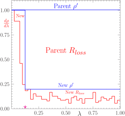
The best cell division is found by examining all $N_{b}-1$ end-points $\lambda=q+ih/N_{b}$, $i=1,2,...,N_{b}-1$ of the bins in the histogram, as a possible candidate for the division point (plane in two and more dimensions) between the two daughter cells, and choosing the best one. In the right-hand part of Fig. 8 we have marked such a candidate division point with a star. For a given division point, we determine for two daughter cells the new “ceiling function” $\rho^{\prime}$; in Fig. 8 it is the line marked “New $\rho^{\prime}$”. For each daughter cell we evaluate $R_{loss}$. The summary $R_{loss}$ for both daughter cells is easily recognized as an area between the line marked “New $\rho^{\prime}$” and the histogram. Of course, we automatically get the new total $R_{loss}$ smaller than for the original parent cell! This procedure is repeated for all possible $j=1,2,...,N_{b}-1$ division points and each time we record the net gain in $\Delta_{j}R_{loss}=R_{loss,parent}-R_{loss,daughter1}-R_{loss,daughter2}$. For the actual best division point we chose the division point with the largest gain $\Delta_{j}R_{loss}$. In Fig. 8 the star marks the best division point.

Figure 9: Two-dimensional $\rho(\vec{x})$ (left) and the geometry of the first three simplical cells (right). Inside the area marked by the inset rectangle $\rho(\vec{x})=0$.

Figure 10: Distributions used in the construction of $\lambda_{div}$ in the case of optimizing the maximum weight.

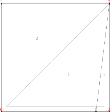
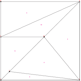
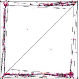
Let us now consider the 2-dimensional distribution $\rho(x)$ depicted in the left part of Fig. 9, which is non-zero within the narrow strip along the four edges of the rectangle. In the simplical mode Foam divides starting $n$-dimensional hyperrectangle into $n!$ simplices – in this case into two triangles. We concentrate on the division procedure of the lower triangle; see the right part of Fig. 9. In the exploration of this triangular cell we use 1000 MC points and project them onto three edges. The corresponding three histograms are shown in Fig. 10, where the middle histogram represents the projection onto the diagonal – this is why it features two distinct peaks at the ends. In all three plots we have also drawn the curve for $\rho^{\prime}(x)$ for the best hypothetical split. The most promising split in terms of the gain in $R_{loss}$ turn outs to be related to the middle plot and is marked in the right part of Fig. 9.

The reader may notice that the $\rho^{\prime}(x)$ in the middle plot of Fig. 10 is not of the type discussed above, because it has two discontinuities instead of one. This is because in Foam we have introduced an important refinement of the algorithm to find an optimal $\lambda_{div}$. One may easily notice that the algorithm described above could not correctly locate the drop in the distribution $d\rho/d\lambda$ of the middle plot, because there are two equally strong peaks at the ends of this distribution. In the improved version of the algorithm the search of the optimal $\lambda_{div}$ uses all pairs of the bin edges $(\lambda_{i},\lambda_{j})=(q+ih/N_{b},\;q+jh/N_{b})$, $0\leq i<j\leq N_{b}$. For every pair $(i,j)$ a new ceiling function $\rho^{\prime}(x)$ is determined, such that it is unchanged outside the subinterval $(\lambda_{i},\lambda_{j})$ and is “majorizing” the histogram bins inside this subinterval. Once we find out the best pair $(i,j)$ in terms of $R_{loss}$, then we take either $\lambda_{i}$ or $\lambda_{j}$ as a division point $\lambda_{div}$ (at least one of them is not equal to 0 or 1). In the case of two or more peaks in $d\rho/d\lambda$ the resulting division point $\lambda_{div}$ happens to be close to one of the edges of the gap between the two peaks. This feature prevents the Foam algorithm (at least partly) from placing a new division plane across a void in the multidimensional distribution $\rho(x)$. In other words such a void will “repel” the division hyperplanes. In the case of the double peak structure in the middle plot of Fig. 10, the improved algorithm will of course allocate the big value of $R_{loss}$ to a new cell (interval), which includes the gap. In the next step of the foam build-up this cell (interval) will have a big chance to be split, and for this split the position of the split point will be located at the second edge of the gap. This is exactly what we need for an efficient foam evolution.

Figure 11: Distributions used in the construction of $\lambda_{div}$ in the case of optimizing the variance.

3.4.2 Optimization of the variance – choosing $\lambda_{div}$

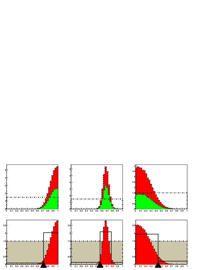
Let us consider now the case of finding out the best $\lambda_{div}$ for $R_{loss}$ corresponding to optimization of the variance. The strategy is again to choose $\lambda_{div}$ by minimizing $R_{loss}$. In Fig. 11 we illustrate our algorithm on the example of the three projections of the triangular cell. The three projections correspond to a triangular cell in two dimensions. (We do not specify $\rho(x)$, as it is irrelevant for the purpose of our explanation.) In the upper row of the three plots in Fig. 11 we show as a horizontal line the value of the distribution $\rho_{loss}=\sqrt{\langle\rho^{2}\rangle}$ (it is the same for all three projections). The solid histogram is the distribution $d\rho/d\lambda$ and the dashed histogram is the distribution $d\rho_{loss}/d\lambda$ calculated bin by bin using $\sqrt{\langle\rho^{2}\rangle}$, treating every bin as a separate cell. The properly normalized difference of the above two distributions $\sqrt{\langle\rho^{2}\rangle}-\langle\rho\rangle$ is plotted separately as the dashed histograms in the lower row of the three plots in Fig. 11. The horizontal line for the total $\rho_{loss}$ is shown once again there. The histogram of $d\rho_{loss}/d\lambda$ gives us an idea, where the biggest source of the variance is located and our aim is to “trap” it properly with an intelligent choice of $\lambda_{div}$. We follow an algorithm similar to that of the maximum weight minimization, namely we loop over pairs of the bin edges $(\lambda_{i},\lambda_{j})=(q+ih/N_{b},q+jh/N_{b})$, $0\leq i<j\leq N_{b}$, and for every pair we calculate $R_{loss}$ inside the interval $(\lambda_{i},\lambda_{j})$ and outside it. We find out which $(i,j)$ provides the biggest gain $\Delta_{ij}R_{loss}=R_{loss,parent}-R_{loss,Inside}-R_{loss,Outside}$. In the lower row of the plots in Fig. 11 we show as a solid line the distribution of $R_{loss}$ for the best pair $(i,j)$. Depending on the peak structure, at least one of the division points of the optimal pair $(\lambda_{i},\lambda_{j})$ is different from 0 or 1, and we take this one as $\lambda_{div}$. In Fig. 11 the chosen $\lambda_{div}$ are marked with black triangles. The above procedure is done for each edge, and the best $\Delta_{ij}R_{loss}$ is used as a guide to define an edge for which the next cell division will be executed. The information about the best edge and the best division point $\lambda_{div}$ is recorded in the cell object. As seen in Fig. 11, $\lambda_{div}$ tends to fall at the position where $d\rho_{loss}/d\lambda$ drops or increases sharply. Note that since the division point is always at the edge of the bin, it is therefore a rational number, $\lambda_{div}=j/N_{b}$. This has interesting consequences, since the number of the bins $N_{b}$ is fixed, it is therefore sufficient to memorize this integer index $j$ (2 Bytes) together with the integer index of the division cell edge (also 2 Bytes) as an attribute of the cell, in order to define fully and uniquely the geometry of the division of the cell! See Section 2.6 for more details on how this is exploited to save the computer memory needed to encode the entire foam of cells.

Figure 12: Examples of the 2-dimensional foam. Number of cells from 10 to 2500.

Figure 13: Example of $\rho(x)$ for which the Foam algorithm of cell division fails.

3.4.3 Concluding remarks on the cell division algorithm

The algorithm of the split of the cell is the important and most sophisticated part of the new Foam. Let us therefore add a couple of final remarks:

• The new, much improved procedure of the choice of the division plane is the most significant difference with respect to Foam 1.x of Ref. [1].

• The choice of the edge based on the histograms for each edge makes sense if we use histograms with at least 2–4 bins and at least 100 MC events per cell. This might be a serious limitation for these $\rho(x)$, which require a lot of CPU time per function call.

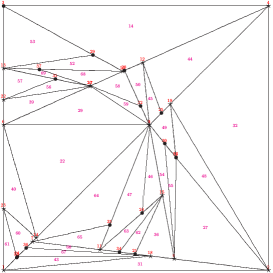
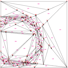
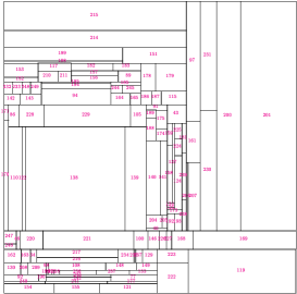
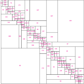
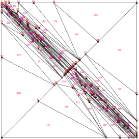
Finally, in Fig. 12 we show examples of the evolution of the foam of cells as the number of the cells grows gradually. The 2-dimensional case is easily visualized and we show it in Fig. 12 for triangular and rectangular cells. In the upper six plots, $\rho(x)$ features a circular ridge, in the bottom two plots it is concentrated along the antidiagonal $x_{1}+x_{2}=1$, the last one corresponding to the $\rho(x)$ of Fig 9.

3.5 Limitations

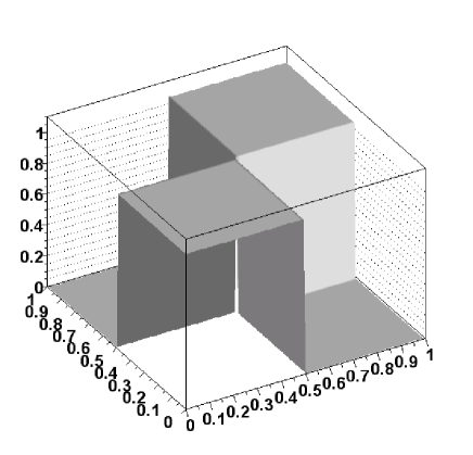
We are aware that the present procedure of selecting the next cell for the split and the procedure of defining the division plane, although quite sophisticated, is not a perfect one and has certain shortcomings. Some of them can probably be corrected for, but some of them are inherent to the method. In Fig. 13 we show a surprisingly simple example of a function for which our method of finding a good division point $\lambda_{div}$ fails. It fails simply because both projections of $\rho(x)$ onto two edges of the rectangle are just flat and our procedure will pick up some $\lambda_{div}$ randomly within $(0,1)$, while the most economic division point is in the middle $\lambda_{div}=1/2$. On the other hand, although the Foam algorithm gets disoriented for the first division, it will recover and correct for the false start in the next divisions rather quickly. It will eliminate the two voids from its area of interest.

Let us notice that the distribution of Fig. 13 violates maximally the “principle of factorizability” $\rho(\vec{x})=\prod_{1}^{n}\rho_{i}(x_{i})$, the principle on which the VEGAS family of the programs is built [3, 4, 5]. Contrary to VEGAS the problem with factorizability in Foam is not a general one, but is limited to a single cell and usually goes away after the cell split. Nevertheless, the algorithm of Foam analysing projections on all edges in a single cell is relying on the “principle of factorizability”.

Class	Short description
TFOAM_INTEGRAND	Abstract class (interface) for the Foam integrand distribution $\rho(x)$
TFVECT	Class of vectors with dynamic allocation of the components. Used in TFOAM and TFCELL
TFMATRIX	Square matrices, used for simplical geometry in the foam
TFPARTITION	Auxiliary small class for looping over partitions and permutations
TFCELL	Class of objects presenting single cell used in TFOAM (Cartesian product of the simplex and hyperrectangle)
TFOAM	Main class of Foam. The entire MC simulator
TPSEMAR	Marsaglia etal. random number generator[23].
TFHST	Simple class of one-dimensional histograms. Used only in the Foam version without ROOT
TFMAXWT	Monitors MC weight, measures performance of the MC run
TFDISTR	Collections of distributions $\rho(x)$ for testing Foam

Table 1: Description of C++ classes of Foam.

TFOAM member	Short description
float m_Versiong	Actual version of the Foam (like 2.34)
char m_Date[40]	Release date of the Foam
char m_Name[128]	Name of a given instance of the TFOAM class
int m_nDims	Dimension of the simplical subspace
int m_kDims	Dimension of the hyperrectangular subspace
int m_TotDimg	Total dimension = m_nDim+m_kDim
int m_nCellss	Maximum number of cells
int m_vMax	Maximum number of vertices (calculated)
int m_LastVe	Actual index of the last vertex
int m_RNmax	Maximum number of random numbers generated at once
int m_OptDrives	Type of optimization =1,2 for variance or maximum weight reduction
int m_OptEdges	Decides whether vertices are included in the cell MC exploration
int m_OptPeeks	Type of cell peek =0,1,2 for maximum, random, random2
int m_OptOrds	Root cell is simplex for OptOrd=1, hyperrectangle for OptOrd=2
int m_OptMCells	=1 economic memory for hyperrectangles is on; =0 off
int m_Chats	=0,1,2 chat level in output; =1 for normal output
int m_OptDebug	=1, additional histogram (dip-switch)
int m_OptCu1st	=1, numbering starts with hyperrectangle (dip-switch)
int m_OptRej	=0 for weighted events; =1 for unweighted events in MC generation
int m_nBins	No. of bins in edge histogram for cell MC exploration
int m_nSampls	No. of MC events, when dividing (exploring) cell
int m_EvPerBins	Maximum number of effective ($w=1$) events per bin
int m_nProj	Number of projection edges (calculated)

Table 2: Data members of the TFOAM class. Associated setters and getters marked as superscripts $s$ and $g$.

TFOAM member	Short description
Provision for the multibranching
int *m_MaskDiv	![m_nProj] Dynamic mask for cell division
int *m_InhiDiv	![m_kDim] Flags inhibiting cell division, h-rectang. subspace
int m_OptPRD	Option switch for predefined division, for quick check
TFVECT **m_XdivPRD	!Lists of division values encoded in one vector per direction
Geometry of cells
int m_NoAct	Number of active cells
int m_LastCe	Index of the last cell
TFCELL **m_Cells	[m_nCells] Array of ALL cells
TFVECT **m_VerX	[m_vMax] Array of pointers to vertex vectors
Monte Carlo generation
double m_MaxWtRej;	Maximum weight in rejection for getting $w=1$ events
TFMAXWT *m_MCMonit;	Monitor of the MC weight for measuring MC efficiency
TFCELL **m_CellsAct	!Array of pointers to active cells, constructed at the end of foam build-up
double *m_PrimAcu	!Array of cumulative $\sum_{i=1}^{k}R^{\prime}_{i}$, for cell index generation
TObjArray *m_HistEdg	Histograms of $w$, one for each edge, with ROOT
TObjArray *m_HistDbg	Histograms for debug (m_OptDebug=1), with ROOT
TH1D *m_HistWt;	Histograms of MC weight, with ROOT
TFHST **m_HistEdg	Array of pointers to histograms, without ROOT
TFHST *m_HistWt;	Histograms of MC weight, without ROOT
double *m_MCvectg	[m_TotDim] Generated MC vector for the outside user
double m_MCwtg	MC weight
double *m_Rvec	[m_RNmax] Random number vector from r.n. generator, up to m_TotDim+1 maximum elements
Externals
TFOAM_INTEGRAND *m_Rho${}^{g}s$	The distribution $\rho$ to be generated/integrated
TPSEMAR *m_PseRan${}^{g}s$	Generator of the uniform pseudo-random numbers
Statistics and MC results
long m_nCallsg	Number of function calls
long m_nEffev	Total no. of effective $w=1$ events in build-up
double m_SumWt, m_SumWt2	Sum of weight $w$ and squares $w^{2}$
double m_NevGen	No. of MC events
double m_WtMax, m_WtMin	Maximum/Minimum weight (absolute)
double m_Primeg	Primary integral $R^{\prime}$, ($R=R\langle w\rangle$)
double m_MCresult	True integral $R$ from the cell exploration MC
double m_MCerror	and its error
Working space for cell exploration
double *m_Lambda	[m_nDim] Internal parameters of the simplex: $\sum\lambda_{i}<1$
double *m_Alpha	[m_kDim] Internal parameters of the h-rectang.: $0<\alpha_{i}<1$

Table 3: Data members of the class TFOAM. Cont.

TFOAM method	Short description
Constructors and destructors
TFOAM()	Default constructor (for ROOT streamer)
TFOAM(const char*)	User constructor
T̃FOAM()	Explicit destructor
TFOAM(const TFOAM&)	Copy Constructor NOT USED
TFOAM& operator=(const TFOAM& )	Substitution NOT USED
Initialization, foam build-up
void Initialize(TPSEMAR*,	Initialization, allocation of memory
TFOAM_INTEGRAND*)	and the foam build up
void InitVertices(void)	Initializes first vertices of the root cell
void InitCells(void)	Initializes first $n!$ cells in h-rect. root cell
void Grow(void)	Adds new cells to foam, until buffer is full
int Divide(TFCELL *)	Divides cell into two daughters
void Explore(TFCELL *Cell)	MC exploration of cell main subprogram
void Carver(int&,double&,double&)	Determines the best edge, $w_{\max}$-reduction
void Varedu(double[ ],int&,double&,double&)	Determines the best edge, $\sigma$-reduction
long PeekMax(void)	Chooses one active cell, used in Grow
TFCELL* PeekRan(void)	Chooses randomly one active cell, in Grow
void MakeLambda(void)	Generates random point inside simplex
void MakeAlpha(void)	Generates rand. point inside h-rectangle
int CellFill(int, TFCELL*,
int*,TFVECT*,TFVECT*)	Fills next cell and return its index
void MakeActiveList(void)	Creates table of all active cells
Generation
void MakeEvent(void)	Makes (generates) single MC event
void GetMCvect(double *)	Provides generated random MC vector
void GetMCwt(double &)	Provides MC weight
double MCgenerate(double *MCvect)	All the above in single method
void GenerCell(TFCELL *&)	Chooses one cell with probability $\sim R^{\prime}_{j}$
void GenerCel2(TFCELL *&)	Chooses one cell with probability $\sim R^{\prime}_{j}$
Finalization, reinitialization
void Finalize(double&, double&)	Prints summary of MC integration
void GetIntegMC(double&, double&)	Provides MC integral
void GetIntNorm(double&, double&)	Provides normalization
void GetWtParams(const double,
double&, double&, double&)	Provides MC weight parameters
void LinkCells(void)	Restores pointers after restoring from disk
Debug
void CheckAll(const int)	Checks correctness of the data structure
void PrintCells(void)	Prints all cells
void PrintVertices(void)	Prints all vertices
void LaTexPlot2dim(char*)	Makes LaTeX file for drawing 2-dim. foam
void RootPlot2dim(char*)	Makes C++ code for drawing 2-dim. foam

Table 4: Methods of TFOAM class.

4 The Foam code

At present, the C++ version of the Foam code is more advanced than the Fortran77 version. (We do not plan to develop F77 code any further.) In this section we shall therefore describe mainly the C++ code.

The code of the Foam version 1.x was originally written in Fortran77 with popular language extensions, such as long variable names etc. It was already written in an object-oriented style, as much as it had been possible. In particular the main classes TFOAM and TFCELL of the present C++ version were already present under a certain form. The important shortcoming of the F77 version is the lack of dynamic allocation of the memory. Otherwise, it has most of the functionality of the C++ version; see later in this section for a list of limitations.

4.1 Description of C++ classes

In Table 1 we list all classes of the Foam package. The main class is TFOAM, which is the MC simulator itself. It is served by the class TFCELL of the cell objects, and three auxiliary classes TFVECT, TFMATRIX and TFPARTITION. The other classes are not related directly to the Foam algorithm – they are utilities used by Foam: random-number generator class TPSEMAR [23] and the histogramming class TFHIST. The class TFDIST provides a menu of the distributions for testing Foam. In the following we shall describe in more detail the key classes TFOAM and TFCELL.

4.2 TFOAM class

TFOAM is the main class. Every new instance of this class (properly initialized) is another independent Foam event generator. In Tables 2 and 3 we provide a full list of the data members of the class TFOAM and their short description. As seen in these tables, we have added the prefix “m_” to all names of the data members, so that they are visually different, in the code, from the other variables (which is recommended practice in C++ coding).

Generally, one may notice that many data members could be declared (and allocated) as the local variables in the procedures, instead of being data members. For example, vector m_MCvect, which transpors random numbers out from the random number generator m_PseMar could be declared locally at every place where m_PseMar is called. We opted for a more “static” structure of the data, with more than necessary of the data members in the class, at the expense of the human readability of the code, in order to: (a) facilitate the implementation persistency with ROOT, (b) gain in execution speed and (c) facilitate the translation to other languages.

Most of the methods (procedures) of the class TFOAM are listed in Table 4. We omitted in this table “setters” and “getters”, which provide access to some data members, and simple inline functions, such as sqr for squaring a double variable. Data members which are served by the setters and getters are marked in Tables 2 and 3 by the superscripts “$s$” or/and “$g$”.

Let us now characterize briefly the role of most important methods of the class TFOAM in the Foam algorithm.

Figure 14: Calling sequence of the Foam procedures during the foam build-up (initialization).

4.2.1 Procedures for Foam initialization and foam build-up

The constructor TFOAM(const char*) is for creating an object of the class TFOAM. Its parameter is the name given by the user to an object. The principal role of this constructor is to initialize data members to their default values – no memory allocation is done at this stage. After resetting all kinds of steering parameters of the Foam to preferred values (using setters) the user calls the Initialize method, which builds up the foam of cells. The two methods InitVertices and InitCells allocate arrays of vertices and cells (pointers) with empty cells. The empty cells are allocated/filled using CellFill. Next comes the procedure Grow which loops over cells, picking up the most promising cell for the split, either randomly using PeekRand or deterministically using Peekmax. The chosen cell is split using Divide. It is, however, the procedure Explore called by Divide (and by InitCells for the root cell) which does the most important job in the Foam build-up: it performs a small MC run for each newly allocated daughter cell. It calculates how profitable the future split of the cell will be and defines the optimal cell division geometry with the help of Carver or Varedu procedures, for maximum weight or variance optimization respectively. All essential results of the exploration are written into the explored cell object. At the very end of the foam build-up, MakeActiveList is invoked to create a list of pointers to all active cells, for the purpose of the quick access during the MC generation. The procedure Explore uses two procedures MakeLambda and MakeAlpha, which generate randomly (uniformly) coordinates of the MC points inside a given cell. The above sequence of the procedure calls is depicted in Fig. 14.

4.2.2 Procedures for MC generation

The MC generation of a single MC event is done by invoking MakeEvent, which chooses randomly a cell with the help of procedure GenerCell2 and, next, the internal coordinates of the point within the cell using MakeLambda and/or MakeAlpha. The absolute coordinates of the MC event are calculated and stored in the data member double-precision vector m_MCvect. The MC weight is calculated using an external procedure that provides the density distribution $\rho(x)$, which is represented by the pointer m_Rho. A class to which the object m_Rho belongs must inherit from the abstract class TFOAM_INTEGRAND. The MC event (double-precision vector) and its weight are available through getters GetMCvect and GetMCwt. Note that the variables of the hyperrectangular subspace come first in the m_MCvect, before variables of the simplical subspace.

The user may alternatively call MCgenerate, which invokes MakeEvent and provides a MC event and its weight, all at the same time.

4.2.3 Procedures for finalization and debugging

The use of the method Finalize is not mandatory. It prints statistics and calculates the estimate of the integral using the average weight from the MC run. The amount of printed information depends on the values of m_chat. For the normalization of the plots and integrals, the user needs to know the exact value of $R^{\prime}=\int\rho^{\prime}(x)dx$, which is provided by the method GetIntNorm or Finalize. The actual value of the integrand from the MC series is provided by GetIntegMC. Note that for the convenience of the user GetIntNorm provides $R^{\prime}$ or MC estimate of $R=\int\rho(x)dx$, depending on whether the MC run was with weighted or $w=1$ events.

Another useful finalization frocedure,

GetWtParams(const double eps, double &AveWt, double &WtMax, double &Sigma)

provides three parameters that characterize the MC weight distribution: the average weight AveWt, the “intelligent” maximum weight WtMax $=w^{\varepsilon}_{\max}$ for a given value of eps $=\varepsilon$ (see Sect. 6 for its definition) and the variance sigma $=\sigma$. In particular, in the case of unweighted events, $w^{\varepsilon}_{\max}$ can be used as an input for the next MC run.

The Foam program includes procedure CheckAll, which checks the correctness of the pointers in the doubly linked tree of cells (this can take time for large $N_{c}$). It can sometimes be useful for debugging purposes. Another two methods PrintVertices and PrintCells can be used at any stage of the calculation in order to print the list of all cells and vertices. In the case of the two-dimensions there is a possibility to view the geometry of the cells with a 2-dimensional plot, which is either a LaTeX file produced by LaTexPlot2dim, or a ROOT file produced by RootPlot2dim.

TCELL member	Short description
“Static” members, the same for all cells!
short int m_kDim	Dimension of hyperrectangular subspace
short int m_nDim	Dimension of simplical subspace
short int m_OptMCell	Option of economic memory for usage (hyperrectangular subspace)
short int m_OptCu1st	=1, Numbering of dims starts with hyperrectangles; =0 simplices
int m_nVert	No. of vertices in the simplex = m_nDim+1
TFCELL **m_Cell0	! Pointer of the root cell
TFVECT **m_Vert0	! Pointer of the vertex list
Linked tree organization
int m_Serial	Serial number (index in m_Cell0)
int m_Status	Status (active or inactive)
int m_Parent	Pointer to parent cell
int m_Daught0	Pointer to daughter 1
int m_Daught1	Pointer to daughter 2
The best split geometry from the MC exploration
double m_Xdiv	Factor $\lambda$ of the cell split
int m_Best	The best edge candidate for the cell split
Integrals of all kinds
double m_Volume	Cartesian volume of this cell
double m_Integral	Integral over cell (estimate from exploration)
double m_Drive	Driver integral $R_{loss}$ for cell build-up
double m_Primary	Primary integral $R^{\prime}$ for MC generation
Geometry of the cell
int *m_Verts	[m_nVert] Pointer to array of vertices in simplical subspace
TFVECT *m_Posi	Pointer to position vector, hyperrectangular subspace
TFVECT *m_Size	Pointer to size vector, hyperrectangular subspace

Table 5: Data members of the class TFCELL.

4.3 TFCELL class

TFCELL is an important class of objects representing a single cell of the foam. Data members of the class are listed in Table 5.

Most of the methods of the TFCELL class are setters and getters. The non-trivial methods are GetHcub and GetHSize, which calculate the absolute position and size of hyperrectangles in the algorithm of Section 2.6, and MakeVolume, which calculates the Cartesian volume of the cell. In the simplical subspace, the volume is a determinant of a square matrix of the class TFMATRIX.

4.4 Persistency with the help of ROOT

The C++ language does not provide any built-in mechanism of the persistency of the classes. For this purpose we use the ROOT package [16], with the help of its “automatic streamers”. ROOT is a useful C++ library for histogramming, organizing large databases of identical objects of the type used in high energy physics experiments. It also provides an efficient input/output, with compressing capabilities.

Providing full persistency for C++ classes preserving all the structures of the pointers is not a trivial task in general. ROOT can do it, even for pointers. For this, our code had to be reorganized slightly: puting additional directives for ROOT in the comment lines, remooving static variable, explicit integer indices instead of pointers in some places. As a whole, this solution is relatively simple, and works correctly. In Tables 2 and 3 we have at the beginning of the description certain characteristic marks which are directives for the persistency mechanism of ROOT, see the ROOT manual [16] for more details.

One has to remember, when reading a TFOAM class object from the disk, that the method LinkCells() has to be invoked in order to fully reconstruct all pointers in the doubly linked tree of cells. Moreover, any object of the class TFOAM restored from the disk file will have its internal object for the random number generator and distribution function. There is a method that provides access (pointer) to these objects, if necessary. The relevant fragment of the code may look as follows:

 TPSEMAR *RNGen= FoamX->GetPseRan();        //get pointer of RN generator
 TFDISTR *RHO  = (TFDISTR*)FoamX->GetRho(); //get pointer of distribution

It might be useful if, for instance, one wants to reinitialize the random number generator used by the TFOAM class object, which has been read from the disk file, with a new “random seed”.

Foam can be used with or without ROOT. In the code all parts of the code dependent on ROOT enclosed in the pair of preprocessor commands #ifdef ROOT_DEF ... #endif, where the ROOT_DEF environmental variable is defined centrally in the header file ROOT_DEF.h. Eliminating ROOT requires removing this variable and modifying makefile accordingly (the TFHST class has to be linked). The version without ROOT does not feature persistency, and is employing its own simple histogramming class TFHST instead of the ROOT class TH1D. ROOT also helps to create documentation of the Foam in the html format. We recommend a version tied up with ROOT.

4.5 Fortran77 version and its limitations

We also provide users with the Fortran77 versions of Foam. There are two of them at the development level 2.02 (May 2001) of the algorithm. In the first one cells can be simplical, hyperrectangular and the Cartesian product of the two. This version is limited to dimension five for the simplical subspace and not very useful for large dimensions ($n\geq 5$) in the hyperrectangular space, because it does not feature the memory-saving algorithm of Section 2.6. Another version, named MCell (standing for Mega-Cell), features only hyperrectangular cells; on the other hand, it includes the memory-saving algorithm described in Section 2.6. We recommend the reader to use the version MCell.

Neither of these versions can have dynamic memory allocation; they have a maximum dimensions of the integration/simulation subspaces (simplical and hyperrectangular) hard-coded in the source code. Any change of these maximum dimensions requires recompilation of the code.

Present versions in Fortran77 are substantially improved with respect to the original version of Ref. [1]. For the option of minimizing the maximum weight, they have exactly the same algorithm (of the cell split) as the C++ version. They feature, however, an older, more primitive version of the algorithm of finding the best cell division for the variance reduction.

The structure of the programs, naming of procedures and variables, configuration parameters and their meaning are very similar in the F77 and C++ versions. Some differences in the usage will be indicated in the next subsections.

4.6 Future development

In the following we indicate some of the possible future developments of the Foam package. As already indicated we do not plan to develop the Fortran77 version any further. On the other hand, it would be interesting to upgrade the existing Foam version 1.x in the JAVA language[2] to the level of the present version 2.x.

As for the C++ version, it would be a logical development to inherit the class of pseudo-random number generators TPSEMAR from a unique abstract class, and in this way to define a universal interface for a library of the number generators. We intend to collect a library of a few random number generators with a universal interface (or find one) for the use in Foam and applications based on it.

Concerning the version of Foam adapted to parallel processing, as in Refs. [5, 8, 9, 10], we do not have plans in this direction in the immediate future. Here, we have of course in mind the use of the true CPU parallelism in the foam of cells build-up. One has to remember that in the high energy physics applications, which are our main objective, the foam of cell build-up will always be a tiny fraction of the total CPU time. The main fraction will be the subsequent MC simulation in which, as the vast experience with PC-farms in CERN and FNAL shows, one may organize the MC simulation with a low level of parallelism, with many simulators started with different random seeds running in parallel but not communicating – another specialized job combines all the results at the very end of the run. However, the first practical examples of true parallelism in the massive MC simulation for the purpose of the high energy physics experiments has appeared recently [24] and is used in the LEP2 data analysis.

The main algorithm of Foam is quite stable at this stage, and the main emphasis in its future development will be on making it more user friendly and better adapted to the use as a part of bigger MC projects. In particular its provisions for multibranching will become more sophisticated, as more feedback comes from real-life applications.

5 Usage of Foam

In the following we provide basic information on how to use the Foam program in the user application.

5.1 Foam distribution directory of the C++ version

The Foam package is distributed together with the demonstration main programs and some utilities in the form of about 20 files in a single UNIX directory FOAM-export-v2.05. Demonstration runs can be executed using standard make commands as follows:

       make Demo-run
       make DemoPers
       make Demo-map
       make DemoNR-run

The essential fragments of the output from running command “make Demo-run” are shown in Appendix B. The compilation and linking procedure is encoded in the file Makefile, and it has to be checked by the user whether it conforms to the local operating system. In particular, if ROOT is used, then certain paths and environmental variables in Makefile have to be adjusted. The use of ROOT is decided by the presence of the variable ROOT_DEF in the file ROOT_DEF.h. Without ROOT, the user should execute command “make DemoNR-run”.

The essential part of Foam, that is class TFOAM, TFCELL and a few auxiliary classes, is located in the files TFOAM.cxx and TFOAM.h. This is the “core” of the Foam source. The source code of the other utility classes TFHST, TFMAXWT, TPSEMAR and TFDISTR are in separate files. The main programs are in files Demo.cxx and DemoPers.cxx. They should serve as a useful template for the user’s own application based on Foam.

There is also one Fortran77 source code, circe2.f, which contains a testing density distribution (2-dimensional beamstrahlung spectrum [25] of the electron linear collider [26]) used in TFDISTR. The Makefile provides, therefore, also a useful example of linking C++ and F77 codes.

There are also two output files output-Demo.linux and output-DemoNR.linux, which the reader may use to check whether he is able to reproduce these benchmark output results.

5.2 Simple example of an application

A very simple example of the use of Foam may look as follows:

//   *** Initialization ***
double MCwt;
TFDISTR *Density1 = new TFDISTR(FunType); // Create integrand function
TPSEMAR *PseRan   = new TPSEMAR();        // Create random numb. generator
TFOAM   *FoamX    = new TFOAM("FoamX");   // Create Simulator
FoamX->SetkDim( 3);                       // Set dimension, h-rect.
FoamX->Initialize(PseRan,  Density1 );    // Initialize simulator
//   *** MC Generation ***
TFHST *hst_Wt = new TFHST(0.0,1.25, 25);  // Create weight histogram
double *MCvect =new double[3];            // Monte Carlo event
for(long loop=0; loop<1000000; loop++){
   MCwt = FoamX->MCgenerate(double *MCvect); // Generate MC event
   hst_Wt->Fill(MCwt,1.0);                   // Fill weight histogram
}
//   *** Finalization ***
double IntNorm, Errel;
FoamX->Finalize( IntNorm, Errel);  // Print statistics, get normalization
double MCresult, MCerror, AveWt, WtMax, Sigma;
FoamX->GetIntegMC( MCresult, MCerror);        // get MC integral
double eps = 0.0005;
FoamX->GetWtParams(eps, AveWt, WtMax, Sigma); // get MC wt parameters
hst_Wt->Print();                   // Print weight histogram

The user normally provides his own density distribution function belonging to the class that has to inherit from the following abstract class:

class TFOAM_INTEGRAND{ // Abstract class of distributios for Foam
 public:
  TFOAM_INTEGRAND() { };
  virtual ~TFOAM_INTEGRAND() { };
  virtual double Density(int ndim, double*) = 0;
};

In the above example the distribution *Density1 belongs to the class TFDISTR, which is provided in the Foam distribution directory.

Param.	Value	Meaning
nDim	0∗	Dimension of the simplical subspace
kDim	0∗	Dimension of the hyperrectangular subspace
nCells	1000∗	Maximum number of cells,
nSampl	200∗	No. of MC events in the cell MC exploration
nBin	8∗	No. of bins in edge-histogram in cell exploration
OptRej	0∗	OptRej = 0, weighted; =1, $w=1$ MC events
OptDrive	2∗	Maximum weight reduction
	1	or variance reduction
OptPeek	0∗	Next cell for split with maximum $R^{\prime}_{I}$ (PeekMax)
	1	or randomly with probability $\sim R^{\prime}_{I}$ (PeekRan)
OptEdge	0∗	Vertices are NOT included in the cell MC exploration
	1	or vertices are included in the cell MC exploration
OptOrd	0∗	Root cell is a hyperrectangle in simplical subspace
	1	or root cell is a simplex in simplical subspace
OptMCell	1∗	Economic memory algorithm in hyperrectangular subspace is ON
	0	or economic memory algorithm in hyperrectangular subspace is OFF
EvPerBin	25∗	Maximum number of effective $w=1$ events/bin
	0	or counting of number eff. events/bin is inactive
Chat	1∗	=0,1,2 is the “chat level” in the standard output
MaxWtRej	1.1∗	Maximum weight used to get $w=1$ MC events

Table 6: Fourteen principal configuration parameters and switches of the Foam program. The default values are marked with the star superscript.

5.3 Configuring Foam

Foam has fourteen principal configuration parameters plus parameters inhibiting and/or predefining the division geometry in the cell split.

5.3.1 Principal configuration parameters

All of the principal parameters listed in Table 6 are set to meaningful default values, hence the beginner may stay ignorant of their role for some time, and learn gradually how to exploit them in order to improve the efficiency of Foam in the actual application. All these parameters are data members of the TFOAM class, see Table. 2. If the user wants to redefine all of them, then the relevant piece of code will look as follows:

  FoamX->SetnDim(     nDim);
  FoamX->SetkDim(     kDim);
  FoamX->SetnCells(   nCells);
  FoamX->SetnSampl(   nSampl);
  FoamX->SetnBin(     nBin);
  FoamX->SetOptRej(   OptRej);
  FoamX->SetOptDrive( OptDrive);
  FoamX->SetOptPeek(  OptPeek);
  FoamX->SetOptEdge(  OptEdge);
  FoamX->SetOptOrd(   OptOrd);
  FoamX->SetOptMCell( OptMCell);
  FoamX->SetEvPerBin( EvPerBin);
  FoamX->SetMaxWtRej( MaxWtRej);
  FoamX->SetChat(     Chat);

In practical applications one will redefine only some of them. The minimum requirement is that the user sets a non-zero value of nDim or kDim such that the total dimension nDim+kDim is a non-zero positive integer.

5.3.2 Inhibiting cell division in certain directions

If the user of Foam decides to inhibit the division in certain variable in the hyperrectangular subspace, this can be done with the method SetInhiDiv(int iDim, int InhiDiv) of the class TFOAM, where iDim is the dimension index for which inhibition is done and InhiDiv is the inhibition tag. This method should be used before invoking Initialize, after setting nDim and/or kDim. The relevant code may look as follows:

  FoamX->SetInhiDiv(0, 1); //Inhibit division of x_1
  FoamX->SetInhiDiv(1, 1); //Inhibit division of x_2

The allowed values are InhiDiv=0,1 and the default value is InhiDiv=0. Note that the numbering of dimensions with iDim starts from zero and variables of the hyperrectangular subspace always come first, before the simplical ones.

5.3.3 Setting predefined cell division geometry

The user may predefine divisions of the root cell in certain variables in the hyperrectangular subspace using the method SetXdivPRD(int iDim, int len, double xDiv[]). The relevant piece of the user code may look as follows:

  double xDiv[3];
  xDiv[0]=0.30; xDiv[1]=0.40; xDiv[2]=0.65;
  FoamX->SetXdivPRD(0, 3, xDiv);

Again, this should be done before invoking Initialize, after setting nDim and/or kDim.

5.4 Persistency

Persistency of the Foam classes is arranged using “default streamers” of the ROOT [16] package. Writing a TFOAM class object into the disk file rmain.root can be done with the single Write as follows:

  TFile RootFile("rmain.root","RECREATE","histograms");
  ...
  FoamX->Write("FoamX"); //Writing Foam on the disk
  ...
  RootFile.Write();
  RootFile.Close();

The instruction FoamX->Write("FoamX") can be put at any place of the code after the instruction FoamX->Initialize(...), see example of the user code shown in Section 5.2.

Next, in another program, the TFOAM class object can be read from the disk file rmain.root as follows:

  TFile fileA("rmain.root");  // connect disk file
  fileA.cd();
  fileA.ls();                        // optional printout
  fileA.Map();                       // optional printout
  fileA.ShowStreamerInfo();          // optional printout
  fileA.GetListOfKeys()->Print();    // optional printout
  TFOAM  *FoamX = (TFOAM*)fileA.Get("FoamX"); // find object
  FoamX->LinkCells();  // restore pointers of the binary tree of cells
  FoamX->CheckAll(1);                // optional x-check of pointers

and at this point the FoamX object is ready to generate MC events, as in the MC generation part of the code shown in Section 5.2.

5.5 Fortran77 versions

The distribution directory FoamF77-2.02-export contains the README file, two demonstration main programs DemoFoam.f and DemoMCell.f to be compiled and run with the help of commands

        make DemoFoam
        make DemoMCell

encoded in the Makefile. The outputs from the above runs can be compared with the benchmark outputs output-DemoFoam-linux and output-DemoMCell-linux.

The basic Foam source files are: FoamA.f with header file FoamA.h and MCellA.f with header file MCellA.h.

For the description of the input (configuration) parameters, see comments in FoamA.f and MCellA.f respectively. The names of the configuration variables are the same as in the C++ version, except nCells, which is here renamed to nBuff. Their values and the meaning are the same.

Demonstration main programs DemoFoam.f and DemoMCell.f can serve as templates for the user application programs.

The testing main program uses the histogramming package GLK of the KKMC program [18], which the user may replace with any other histogramming package.

nDim	kDim	nCalls	nCells	nSampl	$w^{\varepsilon}_{\max}/\langle w\rangle$	$\sigma/\langle w\rangle$	$\Delta_{statist.}R$	$R$
0	1	203719	1000	333	0.99148	0.014585	1.031e-05	0.99999782
0	1	206192	1000	1000	0.99147	0.014752	1.043e-05	0.99999962
0	1	206192	1000	3333	0.99147	0.014752	1.043e-05	0.99999962
0	1	206192	1000	10000	0.99147	0.014752	1.043e-05	0.99999962
0	1	206192	1000	33333	0.99147	0.014752	1.043e-05	0.99999962
0	3	275421	1000	333	0.50538	0.54088	0.000382	0.99986832
0	3	435112	1000	1000	0.50886	0.54033	0.000382	1.00017104
0	3	663493	1000	3333	0.49922	0.55721	0.000394	0.99934710
0	3	834094	1000	10000	0.50359	0.54674	0.000386	1.00056316
0	3	1015157	1000	33333	0.51091	0.54035	0.000382	0.99983999
0	3	2312759	10000	333	0.72346	0.27758	0.000196	0.99977045
0	3	2675820	10000	1000	0.72677	0.27504	0.000194	0.99995080
0	3	3054404	10000	3333	0.72199	0.27710	0.000195	1.00013270
0	3	3333479	10000	10000	0.72200	0.27720	0.000196	1.00008994
0	3	3575366	10000	33333	0.72243	0.27786	0.000196	0.99997875
0	4	3825046	10000	1000	0.50363	0.51168	0.000361	1.00013082
0	4	6559430	10000	10000	0.50297	0.51001	0.000360	0.99960319
2	2	4493961	10000	1000	0.43076	0.63185	0.000446	1.00072564
2	2	9374351	10000	10000	0.44922	0.60669	0.000429	1.00013171
4	0	6642202	10000	1000	0.21029	1.19420	0.000844	1.00072248
4	0	12337748	10000	10000	0.20817	1.20067	0.000849	1.00020405
0	6	2311881	1000	3333	0.04199	2.12091	0.001499	0.99856206
0	6	5542146	1000	10000	0.03847	2.38588	0.001687	0.99912901
0	6	12844256	1000	33333	0.03279	2.61028	0.001845	0.99799089
0	6	12737314	10000	3333	0.15385	1.15211	0.000814	1.00039754
0	6	24134694	10000	10000	0.15313	1.19596	0.000845	0.99945766
0	6	42827237	10000	33333	0.14168	1.22627	0.000867	0.99954178
0	6	42808972	100000	1000	0.30910	0.71250	0.000503	0.99972833
0	6	61803017	100000	3333	0.30805	0.71462	0.000505	1.00002674
0	6	92531875	100000	10000	0.30905	0.71423	0.000505	0.99985093
0	9	78325890	100000	1000	0.03718	1.64608	0.001163	0.99367339
0	9	167710365	100000	3333	0.05247	1.73063	0.001223	1.00109792
0	9	353943409	100000	10000	0.05196	1.80538	0.001276	1.00196909
0	9	272162624	400000	1000	0.08490	1.30193	0.000920	1.00065580
0	9	495260998	400000	3333	0.09174	1.35307	0.000956	0.99884358
0	9	924011087	400000	10000	0.08853	1.38579	0.000979	1.00052122
0	12	261911066	100000	3333	0	5.83954	0.004129	0.97304842
0	12	671460574	100000	10000	0.00640	3.85823	0.002728	0.98878698
0	12	913072065	400000	3333	0.01285	2.73991	0.001937	0.98688299
0	12	2117963809	400000	10000	0.01235	2.92642	0.002069	0.99301117

Table 7: Numerical results of Foam with the maximum weight reduction. Variable nCalls is the total number of the function calls in the foam build-up.

nDim	kDim	nCalls	nCells	nSampl	$w^{\varepsilon}_{\max}/\langle w\rangle$	$\sigma/\langle w\rangle$	$\Delta_{statist.}R$	$R$
0	4	3855289	10000	1000	0.27659	0.31944	0.000225	1.00025027
0	4	7760907	10000	10000	0.30313	0.31483	0.000222	0.99978048
2	2	4589024	10000	1000	0.23086	0.38050	0.000269	0.99967167
2	2	8696153	10000	10000	0.24696	0.37153	0.000262	0.99959278
4	0	6157799	10000	1000	0.08498	0.92314	0.000652	1.00006553
4	0	10547749	10000	10000	0.09881	0.89859	0.000635	1.00024727

Table 8: Numerical results of Foam with the variance reduction.

Figure 15: Testing distribution $\rho_{camel}(x)$ of Ref. [3] in two dimensions.

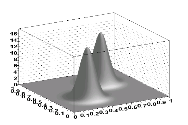
6 Numerical studies and example applications

In the following subsection we examine MC efficiency of the Foam in a series of numerical exercises. In some of them we shall also show examples of the Foam application with the distributions relevant to everyday practice in high energy physics.

6.1 Dependence of the Foam efficiency on the configuration parameters

As a first numerical exercise, we examine the dependence of the Foam efficiency on the most important (input) configuration parameters, including the dimension of the space.

In Table 7 we collect results from many MC runs for various dimensions, numbers of cells and numbers of MC events in single cell exploration, varying also the type of the cells. We always use the same test distribution $\rho_{camel}(x)$ as in Ref. [3], which features two relatively narrow gaussian peaks placed on the diagonal. The 2-dimensional version of this distribution is shown in Fig. 15. We have used the non-default values nBin=4 and EvPerBin=50 and the default values for the other configuration parameters. In this table all tests were done for the default option of reduction of the maximum weight, OptDrive=2 (for results with OptDrive=1, see next table). The efficiency $w^{\varepsilon}_{\max}/\langle w\rangle$ is calculated using maximum weight $w^{\varepsilon}_{\max}$ defined as in Ref. [1] for $\varepsilon=0.0005$. The maximum weight $w^{\varepsilon}_{\max}$ is calculated with the help of the small auxiliary class TFMAXWT.

In Table 7 the efficiency of the MC run measured in terms of $w_{\max}/\langle w\rangle$ and $\sigma/\langle w\rangle$. The value of the integral $R\pm\Delta_{statist.}R$, shown in the last four columns, was obtained from the MC run in which the total number of MC events was $2\times 10^{6}$. The value of the integral $R$ is well known, it is equal to 1, within $10^{-5}$.

The following observations based, on the results of Table 7, can be made:

• Looking at the results, for total dimension $n=4$ we see that the hyperrectangular cells clearly provide better MC efficiency than simplical ones. All other results are for hyperrectangular cells.

• All of the results support the observation that the MC efficiency depends critically on the number of cells. In particular, see results for $n=6$, the increase of nSamp (No. of MC events in cell exploration) beyond a certain value does not help at all.

• In the case of the very inefficient Foam, see $n=12$ with $\sigma/\langle w\rangle\sim 6$, the estimate of the MC statistical error can be misleading. We see an indication that one should not trust runs with $\sigma/\langle w\rangle>3$.

• For this particular testing function the dimension $n=12$ requires a minimum of 400k cells and resulting MC efficiency of order of 1% is barely acceptable.

In Table 8 we repeat the exercise of Table 7 for the option of the variance reduction OptDrive=1 at four dimensions. As compared to Table 7 we see a net improvement in the variance and deterioration of the $w^{\varepsilon}_{\max}$. This agrees with the expectations.

Functions at 2-dimens.	Foam 1.01	Simpl.	H-Rect.	VEGAS
$\rho_{a}(x)$ (diagonal ridge)	0.93	0.93	0.86	0.03
$\rho_{b}(x)$ (circular ridge)	0.82	0.82	0.82	0.16
$\rho_{c}(x)$ (edge of square)	0.57	1.00	1.00	0.53
Functions at 3-dimens.	Foam 1.01	Simpl.	H-Rect.	VEGAS
$\rho_{a}(x)$ (thin diagonal)	0.67	0.74	0.66	0.002
$\rho_{b}(x)$ (thin sphere)	0.36	0.47	0.53	0.11
$\rho_{c}(x)$ (surface of cube)	0.37	0.95	1.00	0.30

Table 9: Efficiencies $\langle w\rangle/w^{\varepsilon}_{\max}$ for $\varepsilon=0.0005$. Functions $\rho_{x}(x)$ are the same as in Ref. [1]. Results from Foam are for 5000 cells (2500 active cells) and cell exploration is done for a modest 200 MC events/cell.

	$k$	$n$	$N_{c}$	$N_{s}$	$N_{b}$	$\frac{N_{eff}}{bin}$	nCall	$\frac{\sigma}{\langle w\rangle}$	$\frac{\langle w\rangle}{w^{\varepsilon}_{\max}}$	$R\pm\Delta R$	$\Delta R/R$
1	2	0	1K	1K	4	25	900K	1168.8	0.0	5.40726$\pm$1.99871	0.36963
1	0	2	1K	1K	4	25	169K	0.2272	0.6149	3.14121$\pm$0.00022	7.1$\cdot 10^{-5}$
2	0	2	1K	1K	4	25	215K	0.2962	0.7754	3.14118$\pm$0.00029	9.3$\cdot 10^{-5}$
1	0	2	5K	1K	4	25	656K	0.0639	0.8421	3.14159$\pm$0.00006	2.0$\cdot 10^{-5}$
1	0	2	10K	1K	4	25	1174K	0.0487	0.8877	3.14156$\pm$0.00005	1.5$\cdot 10^{-5}$
1	0	2	1K	10K	4	25	849K	0.1479	0.5920	3.14118$\pm$0.00014	4.6$\cdot 10^{-5}$
1	0	2	5K	10K	4	25	1457K	0.0606	0.8354	3.14150$\pm$0.00006	1.9$\cdot 10^{-5}$
1	0	2	1K	2K	8	25	621K	0.0606	0.8354	3.14195$\pm$0.00026	8.4$\cdot 10^{-5}$
1	0	2	1K	8K	8	100	1671K	0.1048	0.6652	3.14168$\pm$0.00010	3.3$\cdot 10^{-5}$

Table 10: Numerical results of Foam for 2-dimensional distribution of Eq. (26) for $\mu=10^{-6}$. Variation of the configuration parameters: $k=$kDim, $n=$nDim, $N_{c}=$nCells (No. of function calls), $N_{b}=$nBin, $\frac{N_{eff}}{bin}=$EvPerBin. In the first column we mark the type of the weight optimization OptDrive=1,2, for variance or maximum weight reduction. The value of the integral $R$ and its statistical error $\Delta R$ are from MC run of $N_{MC}=10^{7}$ events. $w^{\varepsilon}_{\max}$ is for $\varepsilon=0.0005$. nCalls is the total number of the function calls in the foam build-up.

6.2 Comparison with Foam 1.x and classic VEGAS

In Table 9 we update the comparison of Foam and VEGAS of Ref. [1], adding results for the new hyperrectangular option. The simplical results are now clearly improved with respect to Ref. [1], because of the better cell division algorithm. Generally, the hyperrectangular cell mode provides as good an efficiency as the simplical one. However, one should keep in mind that Foam with hyperrectangular cells is a factor of 2 or more faster in the execution.

6.3 Example of sharply peaked distribution

In Table 10 we examine the dependence of the MC efficiency/error on the various input configuration parameters of Foam. All these numerical results are for the distribution

$$\rho_{g}(x)=\frac{\mu x_{2}}{(x_{1}+x_{2}-1)^{2}+\mu^{2}},$$ (26)

which, for $\mu=10^{-6}$, has a very sharp ridge across the diagonal $x_{1}+x_{2}=1$. This distribution is taken from Refs.[12, 13] and is related to the photon distribution at high energy electron–positron colliders.

Figure 16: Rectangular and triangular foam of 1000 cells for the distribution of Eq. (26).

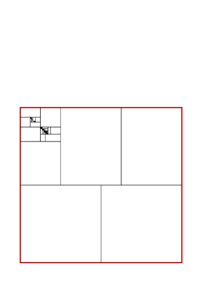
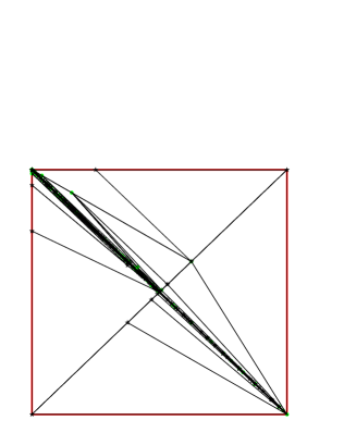
What can we learn from the results in Table 10? First of all, in the first line, we see a spectacular failure of Foam with rectangular cells. The value of the integral is wrong by a factor of 2 and the statistical error is underestimated. This illustrates the problem of the the lack of “angular mobility” of the rectangular cells discussed in Section 2.3; rectangles are unable to align with the singularity along the diagonal.

This we illustrate in the left plot of Fig. 16, for rectangular 1000 cells, where we clearly see “blind spots”. In the right-hand plot the triangular cells in the foam are clearly aligned with the diagonal ridge. In the rows 2 and 3 of Table 10 we see the reasonable numerical results for the triangular foam, which are for the maximum weight reduction and variance reduction options respectively; the other configuration parameters are rather close to the default ones. In rows 4 and 5 we are playing with the increase of the cell number and in the rows 6 and 7 with the number of MC events used in the cell exploration. Finally in rows 8 and 9 we change the binning of the histograms used in the MC cell exploration. As we see, the most profitable in terms of MC efficiency/precision is the increase of the number of cells however, adjusting other parameters can also help. In all cases we display variable nCalls, the number of calls of the density distribution function during the foam build-up. In the best result of line 5 with 10000 triangular cells we have obtained a 5-digit precision for about $10^{7}$ function calls.

Summarizing, we see from the above exercise that the user of Foam has a possibility to adjust several configuration parameters, so that the MC efficiency for a given distribution is improved quite significantly.

MAPPING		$k$	$n$	$N_{c}$	$N_{s}$	$N_{b}$	$\frac{N_{eff}}{bin}$	nCall	$\frac{\sigma}{\langle w\rangle}$	$\frac{\langle w\rangle}{w^{\varepsilon}_{\max}}$	$\Delta R/R$	SIZE
(a1)	OFF	8	0	1	1K	4	25	518	2.1555	0.038	0.00481	15KB
(a2)	ON	9	0	1	1K	4	25	218	1.1391	0.115	0.00254	15KB
(b1)	OFF	8	0	20	1K	4	25	5767	1.1847	0.130	0.00264	15KB
(b2)	ON	9	0	20	1K	4	25	3548	0.7626	0.206	0.00170	15KB
(c0)	OFF	0	8	1000	1K	4	25	487K	1.6603	0.085	0.00371	54KB
(c1)	OFF	8	0	1000	1K	4	25	145K	0.5298	0.359	0.00118	53KB
(c2)	ON	9	0	1000	1K	4	25	125K	0.7626	0.394	0.00104	53KB
(d1)	OFF	8	0	5000	1K	4	25	528K	0.4330	0.438	0.00096	209KB
(d2)	ON	9	0	5000	1K	4	25	596K	0.4037	0.467	0.00090	209KB

Table 11: Numerical results from Foam simulation/integration for the decay process $\tau\to\nu\pi^{-}\pi^{+}\pi^{-}$, according to the matrix element squared of the TAUOLA MC event generator [28, 29]. All MC averages are for 200K events generated after Foam initialization with the configuration parameters given in the table. The notation and the meaning of the quantities are the same as in previous tables. The size of the ROOT disk file, in which the Foam object was written is indicated in the last column.

6.4 Decay of the $\tau$ lepton into 3 pions

In Table 11 we collect numerical results for an example of the application of Foam to the very practical problem of the MC simulation of the decay $\tau\to\nu\pi^{-}\pi^{+}\pi^{-}$, according to the distribution (matrix element squared) taken from the MC program TAUOLA [28, 29].

Figure 17: Feynman diagrams for $\tau$ decay into 3 pions.

Figure 18: The distribution of $\tau\to\nu 3\pi$ decay as a function of $x_{1}$ and $x_{2}$ (without mapping), fixing the other variables to some values.

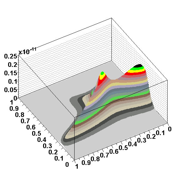
The amplitude of the decay process contains two distinct parts due to two Feynman diagrams, see Fig. 17, which have peaks due to the $a_{1}$ resonance and the $\rho$ resonance. There are two peaks due to $\rho$ resonances that partly overlap in the Lorentz invariant phase-space, such that the actual shape of the differential distribution is rather complicated. We took for this exercise subroutine DPHTRE of TAUOLA, in which nine random numbers are replaced by the nine variables of Foam. The 4-particle phase-space is 8-dimensional. The ninth variable is due to two branches in the phase-space parametrization of TAUOLA, and in case of Foam as well (the method is similar to that of Section 2.11). In cases of “no mapping and no multibranching” we are back to eight dimensions. The variables $x_{1}$ and $x_{2}$ of Foam represent (up to a linear transformation) the two effective masses of the $3\pi$ and $2\pi$ systems. The next four variables $x_{i},i=3,4,5,6$ are the polar variables $\cos\theta$ and $\phi$ of the pions in the rest frame of the $3\pi$ and $2\pi$ systems – this is a completely standard phase-space parametrization, see Ref. [29], and also Ref. [22]. The variables $x_{7}$ and $x_{8}$ are reserved for the overall rotation, and the last one, $x_{9}$, is mapped into branch index $j=1,2$, see Section 2.11. Variables $x_{7}$ and $x_{8}$ are inhibited (no cell-split in them), because the distribution does not depend on them. Variable $x_{9}$ (if present) has a predefined division value equal to $0.5$ and is inhibited for the division (see Section 2.11). In Fig. 18 we show the decay distribution as a function of $x_{1}$ and $x_{2}$ (without mapping), fixing the other variables to some values. The distribution is clearly a non-trivial one.

In Table 11 we show the MC efficiency of Foam for a gradually increasing number of hyperrectangular cells, with the mapping compensating for the Breit–Wigner peaks of the $a_{1}$ and $\rho$ resonances (as in Ref. [29]) and without. One example with simplical cells is also included.

The most striking result in Table 11 is the comparison of lines (a2) and (b1): the Foam algorithm with only 20 cells is performing equally well as the doubly-branched mapping compensating for the resonance peaks of the $a_{1}$ and $\rho$. When going to higher number of cells, the MC efficiency in the cases with and without mapping becomes almost the same. This is expected, since Foam also does the mapping compensating for the resonances on its own. From row (c0) we see also that the simplical mode of Foam is clearly underperforming. We think that Foam configured with 1000 cells, see row (c1) in Table 11, is an economic solution to this particular MC problem. (Mapping due to resonances is not really necessary in this case.)

Figure 19: Foam of rectangular cells for the electron–positron beamstrahlung spectrum of circe2 [25] with 500 cells.

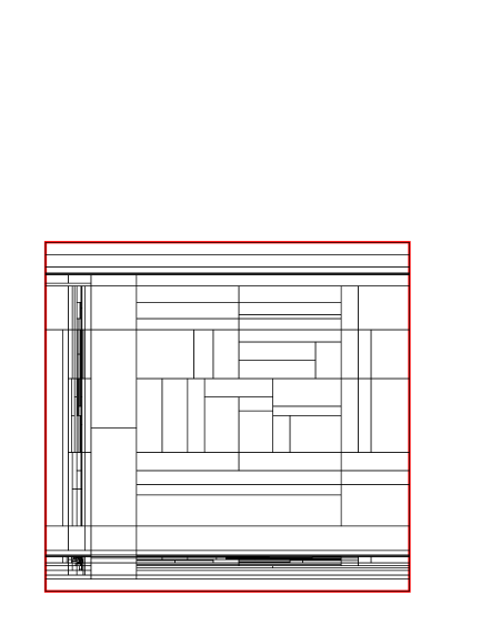
6.5 Beamstrahlung spectrum

In Fig. 19 we show the foam of rectangular cells for the 2-dimensional beamstrahlung spectrum $D(z_{1},z_{2})$ of the electron–positron collider[26] at 500 GeV, encoded in the program circe2 of Refs. [30, 25]. It should be stressed that this spectrum is not known analytically but rather through a numerical fit to results of the machine simulation or (in the future) from an experiment. In order to avoid (integrable) infinite singularities at $z_{i}=1$ in $D(z_{1},z_{2})$ we use the variables $t_{i}=(1-z_{i})^{0.1},\;\;i=1,2$ in Fig. 19. For this exercise we used foam of 500 cells getting the MC efficiency $\sigma/\langle w\rangle=0.41$ and $\langle w\rangle/w^{\varepsilon}_{\max}=0.64$ (for $\varepsilon=0.0005$); enough for practical application (can be easily improved by adding more cells).

Generating $D(z_{1},z_{2})$ is not really such a very much important and difficult problem. A more interesting problem is to generate the distribution $D(z_{1},z_{2})\sigma(sz_{1}z_{2})$, where $\sigma(s)$ is the cross section of some physics process, which may have a strong singularity of its own, such as a resonance or threshold factor. Such a problem was already treated with the help of the Foam program in KKMC [18] event generator and the study of Ref.[31].

7 Conclusions

The author hopes that this new adaptive tool for constructing efficient MC programs will find its way to many applications in high energy physics and beyond. The main points on the new Foam algorithm and the program are the following:

• Foam is a versatile adaptive, general-purpose Monte Carlo simulator.

• The Foam algorithm is based on the cellular division of the integration domain.

• The geometry of the “foam of cells” is rather simple, cells of simplical and/or hyperrectangular shape are constructed in the process of a binary split.

• It works in principle for arbitrary distribution – no assumption of factorizability as in VEGAS of Ref.[3].

• Foam is reducing maximum weight of the weight distribution, it can therefore provide unweighted events. The variance reduction, useful for the integration and generating weighted events, is also available.

• Encoding cells with memory-efficient methods allows up to $\sim 10^{6}$ cells to be built in the computer memory of a typical desktop computer.

• The rules for choosing the next cell for division and the division geometry are based on rather sophisticated analysis of the projection on the cell edges. This costs CPU time, which becomes the main barrier towards higher MC efficiency.

• Foam can deal efficiently with rather strongly peaked distributions, up to relatively high dimensions, $\sim 12$ dimensions, with today’s desktop computers.

Acknowledgements

I would like to thank T. Ohl, A. Para, W. Płaczek, E. Richter-Wa̧s, F. Tkachov and Z. Wa̧s for interesting and useful discussions and R. Brun for help in getting persistency using ROOT. The support and warm hospitality of the CERN Theory Division and DESY Zeuthen is kindly acknowledged. The useful assistance of the Parasoft Company in debugging the C++ code (with the Insure++ tool) is also acknowledged.

Appendix A Variance optimization

Suppose we have already constructed the cells $\omega_{1},\omega_{1},\dots,\omega_{N}$ and within each cell we have defined the function $\rho^{\prime}(x)$ constant over the cell, $\rho^{\prime}(x)=\rho^{\prime}_{I}$. The integral $R^{\prime}_{I}=\int_{\omega_{i}}\rho^{\prime}(x)dx^{n}=\rho^{\prime}_{I}V_{I}$ is known, because the volume of the cell $V_{I}$ is known. The function $\rho(x)$ is not, in general, constant over the cell and the weight $w=\rho(x)/\rho^{\prime}(x)$ is used to determine its integral in the usual way: $R=R^{\prime}\langle w\rangle_{\rho^{\prime}}=\sum_{I}\langle w\rangle_{\rho^{\prime}_{I}}R_{I}$, where the average

$$\langle a\rangle_{\rho^{\prime}_{I}}=\frac{1}{R^{\prime}_{I}}\int_{\omega_{I}}\rho^{\prime}_{I}(x)a(x)dx^{n}$$

is defined for the $I$-th cell alone.

The question is now the following: preserving the geometry of the cells, can we get smaller variance by simply changing the probabilities of the generation of the cells? Rescaling $\rho^{\prime}_{I}\to\rho^{\prime\prime}_{I}=\lambda_{I}\rho^{\prime}_{I}$ does not affect the integral $R$, because the change of the normalization of $R^{\prime}$ and $\langle w\rangle_{\rho^{\prime}}$ is cancelling. It is convenient to assume that the above rescaling preserves $R^{\prime}=R^{\prime\prime}$ and the total average weight $\langle w\rangle_{\rho^{\prime}}=\langle w\rangle_{\rho^{\prime\prime}}$, that is $\lambda_{I}$ obey the constraint $\sum_{I}R^{\prime}_{I}=\sum_{I}R^{\prime}_{I}\lambda_{I}=$ const. With the above constraint in mind, we now ask: for what values of $\lambda_{I}$ is the dispersion of the total weight $\sigma^{2}=\langle w^{2}\rangle_{\rho^{\prime\prime}}-\langle w\rangle_{\rho^{\prime\prime}}^{2}$ minimal? Since by construction $\langle w\rangle_{\rho^{\prime\prime}}$ is independent of $\lambda_{I}$, we may look only for a minimum of $\langle w^{2}\rangle_{\rho^{\prime\prime}}$. With the standard methods we get a (local) minimum condition:

$$\frac{\partial}{\partial\lambda_{I}}\Big{\{}\langle w^{2}\rangle_{\rho^{\prime\prime}}+\Lambda R^{\prime\prime}\Big{\}}=\frac{\partial}{\partial\lambda_{I}}\Bigg{\{}\frac{1}{R^{\prime}}\sum_{I}\int_{\omega_{I}}\left(\frac{\rho(x)}{\rho^{\prime}_{I}\lambda_{I}}\right)^{2}\rho^{\prime}_{I}\lambda_{I}dx^{n}+\Lambda\left(\sum_{I}R^{\prime}_{I}\lambda_{I}\right)\Bigg{\}}=0,$$ (27)

where $\Lambda$ is the Lagrange multiplier. The solution of the minimum condition

$$\frac{R^{\prime}_{I}}{R^{\prime}}\langle w^{2}\rangle_{\rho^{\prime}_{I}}\frac{1}{\lambda_{I}^{2}}-\Lambda R^{\prime}_{I}=0$$ (28)

is simply $\lambda_{I}\simeq{\rm const}\times\sqrt{\langle w^{2}\rangle_{\rho^{\prime}_{I}}}$, or more precisely

$$\lambda_{I}=\frac{\sqrt{\langle w^{2}\rangle_{\rho^{\prime}_{I}}}}{\sum_{J}\frac{R^{\prime}_{J}}{R^{\prime}}\sqrt{\langle w^{2}\rangle_{\rho^{\prime}_{J}}}}.$$ (29)

The value of $\langle w^{2}\rangle_{\min}\equiv\langle w^{2}\rangle_{\rho^{\prime\prime}}$ calculated at the minimum, that is for $\lambda_{I}$ of Eq. (29), is also rather simple

$$\langle w^{2}\rangle_{\min}=\sum_{I}\frac{R^{\prime}_{I}}{R^{\prime}}\;\langle w^{2}\rangle_{\rho^{\prime}_{I}}\;\frac{1}{\lambda_{I}^{2}}=\left(\sum_{J}\frac{R^{\prime}_{J}}{R^{\prime}}\sqrt{\langle w^{2}\rangle_{\rho^{\prime}_{J}}}\right)^{2}=\left(\left\langle\sqrt{\langle w^{2}\rangle_{\rho^{\prime}_{J}}}\;\right\rangle_{\rho^{\prime}}\right)^{2}.$$ (30)

Let us note that the functional $\sqrt{\langle w^{2}\rangle_{\min}}$, which we intend to minimize in the process of the evolution of the foam (cell split) is a simple sum of contributions from all cells. Consequently, when working out details of the split of a given cell we may calculate the gain in terms of the total dispersion independently of other cells, see also below. This very convenient feature is exploited in the algorithm of the foam build-up.

Adopting (temporarily) the following normalization conventions: $\rho^{\prime}_{I}=1$, $w=\rho(x)$ and $R^{\prime}_{I}=V_{I}$, $\lambda_{I}\simeq\sqrt{\langle\rho^{2}\rangle}_{I}$, we get

$$\rho^{\prime\prime}_{I}=\sqrt{\langle\rho^{2}\rangle_{I}},\qquad R^{\prime\prime}_{I}=V_{I}\sqrt{\langle\rho^{2}\rangle_{I}},$$ (31)

where the average $\langle\dots\rangle_{I}$ is understood as defined for points uniformly distributed within the $I$-th cell.

In the Foam algorithm we do not go, of course, through a judicious adjustment of the relative importance of the cells, which minimizes the variance as described above; but instead, we simply declare that the distribution $\rho^{\prime}(x)$ is defined by the optimum solution of Eq. (31). Once we have done that, for the MC weight $w$ defined with respect to such a new $\rho^{\prime}(x)$, we find out that $\langle w^{2}\rangle_{I}=1$ for each cell and, also for all cells, $\langle w^{2}\rangle=1$. What is then minimized in the process of the cell division is the ratio of the variance to the average weight

$$\frac{\sigma^{2}}{\langle w\rangle^{2}}=\left(\frac{R^{\prime}}{R}\right)^{2}-1.$$ (32)

This quantity is not so convenient to optimize in the process of the cell split (foam evolution) and we rather chose to minimize a closely related ‘linearized” quantity

$$R_{loss}=R\left(\sqrt{\frac{\sigma^{2}}{\langle w\rangle^{2}}+1}-1\right)=\sum_{I}V_{I}(\sqrt{\langle w^{2}\rangle_{I}}-\langle w\rangle_{I})=\int\rho_{loss}(x)dx^{n}=R^{\prime}-R,$$ (33)

which is a sum of contributions from all cells and is a monotonous ascending function of $\sigma/\langle w\rangle$. In the process of the cell division $\omega_{I}\to\omega_{Ia}\oplus\omega_{Ib}$, we decrease $\sigma/\langle w\rangle$ step by step, by playing with the geometry of the cell split, so that the gain in the total $R_{loss}=R^{\prime}-R$ due to a given cell split is as big as possible. It is convenient that the contributions from the other cells to $R_{loss}$ are unchanged. In this way every cell split will lead to a smaller and smaller $\sigma/\langle w\rangle$ in the final MC run.

Appendix B Output of the demonstration program in C++

FFFFFFFFFFFFFFFFFFFFFFFFFFFFFFFFFFFFFFFFFFFFFFFFFFFFFFFFFFFFFFFFFFFFFFFFFFFFFFFF
F                                                                              F
F                   ****************************************                   F
F                   ******     TFOAM::Initialize      ******                   F
F                   ****************************************                   F
F                                                      FoamX                   F
F    Version =            2.05   =               Release date:  2002.02.13     F
F       nDim =          0 =  Dimension of the simplical sub-space              F
F       kDim =          2 =  Dimension of the hyper-cubical sub-space          F
F     nCells =       1000 =  Requested number of Cells (half of them active)   F
F     nSampl =        500 =  No of MC events in exploration of a cell cell     F
F       nBin =          8 =  No of bins in histograms, MC exploration of cell  F
F   EvPerBin =         25 =  Maximum No effective_events/bin, MC exploration   F
F   OptDrive =          2 =  Type of Driver   =1,2 for Sigma,WtMax             F
F    OptEdge =          0 =  Decides whether vertices are included in the MC   F
F    OptPeek =          0 =  Type of the cell Peek =0,1 for maximum, random    F
F     OptOrd =          0 =  Root cell hyp-cub. or simplex, =0,1               F
F   OptMCell =          1 =  MegaCell option, slim memory for hyp-cubes        F
F   OptDebug =          1 =  Additional debug histogram, SetDirectory(1)       F
F   OptCu1st =          1 =  Numbering of dimensions  starts with h-cubic      F
F     OptRej =          0 =  MC rejection on/off for OptRej=0,1                F
F   MaxWtRej =               2   =       Maximum wt in rejection for wt=1 evts F
F                                                                              F
FFFFFFFFFFFFFFFFFFFFFFFFFFFFFFFFFFFFFFFFFFFFFFFFFFFFFFFFFFFFFFFFFFFFFFFFFFFFFFFF

FFFFFFFFFFFFFFFFFFFFFFFFFFFFFFFFFFFFFFFFFFFFFFFFFFFFFFFFFFFFFFFFFFFFFFFFFFFFFFFF
F                                                                              F
F                   ***  TFOAM::Initialize FINISHED!!!   ***                   F
F     nCalls =     246799 =            Total number of function calls          F
F     XPrime =       1.2748942   =     Primary total integral                  F
F     XDiver =      0.27441356   =     Driver  total integral                  F
F   MCresult =       1.0004806   =     Estimate of the true MC Integral        F
F                                                                              F
FFFFFFFFFFFFFFFFFFFFFFFFFFFFFFFFFFFFFFFFFFFFFFFFFFFFFFFFFFFFFFFFFFFFFFFFFFFFFFFF

FFFFFFFFFFFFFFFFFFFFFFFFFFFFFFFFFFFFFFFFFFFFFFFFFFFFFFFFFFFFFFFFFFFFFFFFFFFFFFFF
F                                                                              F
F                   ****************************************                   F
F                   ******      TFOAM::Finalize       ******                   F
F                   ****************************************                   F
F     NevGen =       2000 = Number of generated events in the MC generation    F
F     LastVe =         -1 = Number of vertices (only for simplical option)     F
F     nCalls =     248799 = Total number of function calls                     F
F                   ----------------------------------------                   F
F      AveWt =      0.78836949   =     Average MC weight                       F
F      WtMin =   1.3022085e-06   =     Minimum MC weight (absolute)            F
F      WtMax =       1.0227719   =     Maximum MC weight (absolute)            F
F                   ----------------------------------------                   F
F     XPrime =       1.2748942   =     Primary total integral, R_prime         F
F     XDiver =      0.27441356   =     Driver  total integral, R_loss          F
F                   ----------------------------------------                   F
F      IntMC =       1.0050877 +-    0.0052357675  = Result of the MC Integral F
F   MCerelat =    0.0052092644   =     Relative error of the MC intgral        F
F  <w>/WtMax =      0.80037512   =              MC efficiency, acceptance rate F
F  Sigma/<w> =      0.23296539   =              MC efficiency, variance/ave_wt F
F      WtMax =           0.985   =              WtMax(esp= 0.0005)             F
F      Sigma =       0.1836628   =              variance of MC weight          F
F                                                                              F
FFFFFFFFFFFFFFFFFFFFFFFFFFFFFFFFFFFFFFFFFFFFFFFFFFFFFFFFFFFFFFFFFFFFFFFFFFFFFFFF

References

- [1] S. Jadach, Comput. Phys. Commun. 130 (2000) 244, physics/9910004.
- [2] M. Ciesla and M. Slusarczyk, M.Sc. thesis at the Institute of Computer Science, Jagiellonian University, Kraków, Poland, 2000.
- [3] G.P. Lepage, J. Comput. Phys. 27 (1978) 192.
- [4] S. Kawabata, Comput. Phys. Commun. 88 (1995) 309.
- [5] T. Ohl, Comput. Phys. Commun. 120 (1999) 13, hep-ph/9806432.
- [6] G.I. Manankova, A.F. Tatarchenko and F.V. Tkachov, MILXy way: How much better than VEGAS can one integrate in many dimensions?, A Contribution to AINHEP-95, Pisa, Italy, Apr 3-8, 1995 (extended version).
- [7] F. James, Rep. Prog. Phys. 43 (1980) 1145.
- [8] E. de Doncker and A. Gupta, Parallel Computing 24 (1998) 1223.
- [9] E. de Doncker, A. Gupta and R. Zanny, Journal of Computational and Applied Mathematics 112 (1999).
- [10] E. de Doncker, K. Kaugars and A. Gupta, User manual of PARINT1.1, http://www.cs.wmich.edu/parint/.
- [11] S. Jadach and W. Płaczek, Comput. Phys. Commun. 72 (1992) 221.
- [12] K. Tobimatsu and S. Kawabata, A new algorithm fo numerical integration, Research report of Kogakuin University, 1992, No. 72.
- [13] K. Tobimatsu and S. Kawabata, Multi-dimensional integration routine dice for vector processor, Research report of Kogakuin University, 1996, No. 85.
- [14] N. Metropolis et al., J. Chem. Phys. 21 (1953) 1087.
- [15] H. Kharraziha and S. Moretti, Comput. Phys. Commun. 127 (2000) 242.
- [16] R. Brun and F. Rademakers, ROOT - an object oriented data analysis framework, Proceedings AIHENP’96 Workshop, Lausanne, Sept. 1996, Nucl. Inst., Meth. in Phys. Res. A 389 (1997) 81-86, See also http://root.cern.ch/.
- [17] M. Boonekamp, Quark pair simulation near threshold: Reweighting and hadronization, 2001, hep-ph/0111213.
- [18] S. Jadach, B.F.L. Ward and Z. Was, Comput. Phys. Commun. 130 (2000) 260, hep-ph/9912214.
- [19] F.A. Berends, R. Kleiss and S. Jadach, Comput. Phys. Commun. 29 (1983) 185.
- [20] R. Kleiss and R. Pittau, Comput. Phys. Commun. 83 (1994) 141, hep-ph/9405257.
- [21] S. Jadach, Practical guide to Monte Carlo, 1999, physics/9906056.
- [22] M. Skrzypek and Z. Was, Comput. Phys. Commun. 125 (2000) 8, hep-ph/9904385.
- [23] G. Marsaglia, B. Narasimhan and A. Zaman, Comput. Phys. Commun. 60 (1990) 345.
- [24] S. Jadach et al., Comput. Phys. Commun. 140 (2001) 475, hep-ph/0104049.
- [25] T. Ohl, Circe version 2.0: Beam spectra for simulating linear collider and photon collider physics, (to be published, code and parametrisations provided by the author in advance), 2002, WUE-ITP-2002-006.
- [26] ECFA/DESY LC Physics Working Group, J.A. Aguilar-Saavedra et al., (2001), hep-ph/0106315.
- [27] E. de Doncker, R. Zanny and K. Kaugars, Integrand and performance analysis with PARINT/PARVIS, http://www.cs.wmich.edu/parint/, 2000.
- [28] S. Jadach et al., Comput. Phys. Commun. 76 (1993) 361.
- [29] M. Jezabek et al., Comput. Phys. Commun. 70 (1992) 69.
- [30] T. Ohl, Comput. Phys. Commun. 101 (1997) 269, hep-ph/9607454.
- [31] G. Blair, Particle masses and widths via threshold scans at the linear collider, APS/DPF/DPB Summer Study on the Future of Particle Physics (Snowmass 2001), Snowmass, Colorado, 30 June - 21 July 2001.