Statistical Geometry of Packing Defects of Lattice Chain Polymer from Enumeration and Sequential Monte Carlo Method

Abstract

Voids exist in proteins as packing defects and are often associated with protein functions. We study the statistical geometry of voids in two-dimensional lattice chain polymers. We define voids as topological features and develop a simple algorithm for their detection. For short chains, void geometry is examined by enumerating all conformations. For long chains, the space of void geometry is explored using sequential Monte Carlo importance sampling and resampling techniques. We characterize the relationship of geometric properties of voids with chain length, including probability of void formation, expected number of voids, void size, and wall size of voids. We formalize the concept of packing density for lattice polymers, and further study the relationship between packing density and compactness, two parameters frequently used to describe protein packing. We find that both fully extended and maximally compact polymers have the highest packing density, but polymers with intermediate compactness have low packing density. To study the conformational entropic effects of void formation, we characterize the conformation reduction factor of void formation and found that there are strong end-effect. Voids are more likely to form at the chain end. The critical exponent of end-effect is twice as large as that of self-contacting loop formation when existence of voids is not required. We also briefly discuss the sequential Monte Carlo sampling and resampling techniques used in this study.

Keywords: void, lattice model, lattice packing, sequential Monte Carlo.

I Introduction

Soluble proteins are well-packed, their packing densities may be as high as that of crystalline solids [1, 2, 3]. Yet there are numerous packing defects or voids in protein structures, whose size distributions are broad [4]. The volume ($v$) and area ($a$) of protein does not scale as $v\approx a^{3/2}$, which would be expected for models of tight packing. Rather, $v$ and $a$ scale linearly with each other [4]. In addition, the scaling of protein volume and cluster-radius [5] is characteristic of random sphere packing. Such scaling behavior indicates that the interior of proteins is more like Swiss cheese with many holes than tightly packed jigsaw puzzles [4].

What effects do void have? Proteins are often very tolerant to mutations [6, 7, 3, 8], which may suggest potentially stabilizing roles of voids in proteins. Voids in proteins are also often associated with protein function. The binding sites of proteins for substrate catalysis and ligand interactions are frequently prominent voids and pockets on protein structures [9, 10]. However, the energetic and kinetic effects of maintaining specific voids in proteins are not well-understood, and the shape space of voids of folded and unfolded proteins are largely unknown.

In this paper, we examine the details of the statistical nature of voids in simple lattice polymers. Lattice models have been widely used for studying protein folding, where the conformational space of simplified polymers can be examined in detail [11, 12, 13, 14, 15, 16, 17, 18]. Despite its simplistic nature, lattice model has provided important insights about proteins, including collapse and folding transitions [19, 17, 20, 21, 22], influence of packing on secondary structure formation [12, 23], and designability of lattice structures [24, 25]. However, one drawback is that lattice model is not well-suited for studying void-related structural features, such as protein functional sites, since it is not easy to model the geometry of voids.

In this article, we first define voids as topological defects and describe a simple algorithm for void detection in two-dimensional lattice. We then enumerate exhaustively the conformations for all $n$-polymers up to $n=22$, and analyze the relationship of probability of void formation, expected packing density and compactness, as well as expected wall interval of void with chain length. To study statistical geometry of long chain polymers, we describe a Monte Carlo sampling strategy under the framework of Sequential Importance Sampling, and introduce the technique of resampling. The results of simulation of long chain polymers up to $N=200$ for several geometric parameters are then presented. We further explore the conformation reduction factor $R$ of void formation, and describe the significant end-effect of void formation, as well as the scaling law of $R$ and wall interval of voids. In the final section, we summarize our results and discuss effective sampling strategy for studying the conformational space of voids.

II Lattice Model and Voids

Lattice polymers are self-avoiding walks (SAWs), which can be obtained from a chain-growth model [26, 27, 28]. Specifically, an $n$-polymer $P$ on a two-dimensional square lattice ${{{Z}}}^{2}$ is formed by monomers $n_{i},i\in\{1,..,N\}$. The location $x_{i}$ of a monomer $n_{i}$ is defined by its coordinates $x_{i}=(a_{i},b_{i})$, where $a_{i}$ and $b_{i}$ are integers. The monomers are connected as a chain, and the distance between bonded monomers $x_{i}$ and $x_{i+1}$ is $1$. The chain is self-avoiding: $x_{i}\neq x_{j}$ for all $i\neq j$. We consider the beginning and the end of a polymer to be distinct. Only conformations that are not related by translation, rotation, and reflection are considered to be distinct. This is achieved by following the rule that a chain is always grown from the origin, the first step is always to the right, and the chain always goes up at the first time it deviates from the $x$-axis. For a chain polymer, two non-bonded monomers $n_{i}$ and $n_{j}$ are in topological contact if they intersect at an edge that they share. If two monomers share a vertex of a square but not an edge, these two monomers are defined as not in contact.

(Figure 1 here.)

When the number of monomer $n$ is 8 or more, a polymer may contain one or more void (Figure 1a). We define voids as topological features of the polymer. The complement space ${{{Z}}}^{2}-P$ that is not occupied by the polymer $P$ can be partitioned into disjoint components:

$\displaystyle{{{Z}}}^{2}-P=\;V_{0}\;\dot{\cup}\;V_{1}\;...\;\dot{\cup}\;V_{k}.$Here $V_{0}$ is the unique component of the complement space that extends to infinity. We call this the outside. The rest of the components that are disjoint or disconnected to each other are voids of the polymer. Because non-bonded monomers intersecting at a vertex are defined as not in contact, they do not break up the complement space. As an example, the unfilled space contained within the polymer in Figure 1b is regarded as one connected void of size $4$ rather than two disjoint voids of size $2$. A simple algorithm for void detection can be found in Appendix. Figure 2 shows the only six conformations among all 301,100,754 conformations of 22-mer found to have 4 voids.

(Figure 2 here.)

III Voids Distribution by Exact Enumeration

Probability of Forming Voids and Expected Number of Voids.   The number of conformations $\omega(n)$ for $n$-polymer up to $n=25$ by exhaustive enumeration is shown in Table I. The numbers of conformations for polymers up to $n=15$ are in exact agreement with those reported in Chan and Dill [12]. Table I also lists the number of conformations $\omega_{k}(n)$ containing $k=1,2,3$, or $4$ voids.

The probability for a polymer to form one or more voids $\pi_{v}$ is calculated as:

$\displaystyle\pi_{v}=\frac{\sum_{i=1}^{k}\omega_{k}(n)}{\omega(n)}.$The expected number of voids $\bar{n}_{v}$ for a polymer is:

$\displaystyle\bar{n}_{v}=\frac{\sum_{i=1}^{k}\omega_{k}(n)\cdot k}{\omega(n)}.$As the chain length grows, it is clear that both $\pi_{v}$ and $\bar{n}_{v}$ increases (Figure 3a and Figure 3b).

(Figure 3 here.)

Void Size.   The total size $v$ of voids in a polymer is the sum of the sizes of all voids, namely, the total number of all unoccupied squares that are fully contained within the polymer. Let $\omega_{v}(n)$ be the number of conformations of $n$-polymer with total void size $v$. The expected total void size $\bar{v}$ for $n$-polymer is:

$\displaystyle\bar{v}=\frac{\sum_{v}\omega_{v}(n)\cdot v}{\omega(n)}.$Figure 3c shows that the expected void size $\bar{v}$ increases with chain length $n$.

Wall Size of Void.   For a void $V$ of size $v$, what is the required minimum length $l(v)$ for a polymer that can form such a void? Equivalently, what is the size of the wall of the polymer containing void $V$? Here we first restrict our discussion to voids formed only by strongly connected unoccupied sites, namely, any neighboring two sites of a void must be sharing at least one edge of the squares. We exclude voids containing weakly connected sites, where two neighboring sites are connected by only one shared vertex (Figure 1b). For $v=1,2$ and $3$, it is easy from the geometry of the voids to see that $l(v)=8,10$ and $12$, respectively. However, in general $l(v)$ also depends on the shape of the void. A void of size $4$ can have five different shapes. If the void is of the shape of a $2\times 2$ square, $l(4)=12$. For the other four shapes, $l(4)=14$.

For any strongly connected void, we find that the following general recurrence relationship for $l(v)$ holds:

$\displaystyle l(v)=l(v-1)+\left\{\begin{array}[]{cc}2,&{\mbox{if $\Delta\partial V=3$}}\\ 0,&{\mbox{if $\Delta\partial V=2$}}\\ -1,&{\mbox{if $\Delta\partial V=1$}},\\ \end{array}\right.$where $\partial V$ represents the boundary edges of void $V$, and $\Delta\partial V$ represents the net gain in the number of boundary edges introduced by the newly added unoccupied site. Although the number and explicit shapes of strongly connected voids of size up to 5 can be found in [29], there is no general analytical formula known for the number of shapes of a void of size $v$. This is related to the problem of determining the number of polyominos or animals (as in percolation theory) of a given size.

When weakly connected voids are also considered, there are more possible wall sizes for void. For $22$-mer, the number of different wall sizes observed for a void, strongly or weakly connected, at various size are shown in Figure 4a. Voids of size 5 has the largest diversity in wall size. This is of course due to the fixed chain length. A short chain such as the 22mer has only a small number of ways for form large voids. Figure 4b shows the average wall size for various void size in 22-mer. The expected or average wall size $\bar{w}(n)$ for a void in a $n$-polymer can be calculated as:

$\displaystyle\bar{w}(n)=\sum_{v}w\cdot\frac{\omega_{v,w}(n)}{\omega_{v}(n)},$where $v$ is the void size, $w$ the wall size of the void, $\omega_{v,w}(n)$ is the number of $n$-polymers containing a void of size $v$ with wall size $w$, and $\omega_{v}(n)$ is the total number of $n$-polymers with a void of size $v$. Figure 3d shows that $\bar{w}(n)$ increases with chain length. Wall size and void size are analogous to the area and volume of voids in three dimensional space.

Packing Density.   An important parameter that describes how effectively atoms fill space is the packing density $p$. In proteins, it is defined by Richards and colleagues as the amount of the space that is occupied within the van der Waals envelope of the molecule, divided by the total volume of space that contains the molecule [3, 30]. It has been widely used by protein chemists as a parameter for characterizing protein folding [3]. Following this original definition, the packing density $p$ for lattice polymer is:

$\displaystyle p=n/(n+v),$when a $n$-polymer has a total void size of $v$.

The expected packing density $\bar{p}(n)$ for a $n$-polymer can be calculated as:

$\displaystyle\bar{p}(n)=\sum_{p}p\cdot\frac{\omega_{p}(n)}{\omega(n)},$where $\omega(n)$ is the number of all conformations of $n$-mer, $\omega_{p}(n)$ the number of $n$-mers with packing density of $p$. The scaling of $\bar{p}(n)$ with the chain length $n$ decreases roughly linearly between $n=7$ and $n=22$ (Figure 5a). Because it takes at least two additional monomer to increase the size of a void by one, $\bar{p}(n)$ decreases only when $n$ is an odd number for short chains.

Although voids are packing defects, most conformations with voids have high packing density, namely, the total size of voids are small. Among all conformations of 22-mer containing one void, the number of conformation increases monotonically with packing density. The lowest packing density $0.52$ has only $11$ conformations, whereas the highest packing density $0.92$ has the largest number ($6,756,751$) of conformations (Figure 5c). Similar relationship is found among conformations with 2 and 3 voids (Figure5c).

Compactness.   Another important parameter that measures packing of lattice polymer is the number of nonbonded contacts $t$. It is related to the compactness parameter $\rho$, defined in [12] as $\rho=t/t_{\max}$, where $t_{\max}$ is the maximum number of nonbonded contact possible for a $n$-polymer. Compactness $\rho$ has been studied extensively in seminal works by Chan and Dill [12, 23, 31]. Although $p$ is sometimes correlated with the compactness $\rho$, these two parameters are distinct. The relationship between compactness and expected packing density for chain polymer of length $14-22$ is shown in Figure 5. For all chain lengths, both maximally compact polymer ($\rho=1$) and extended polymer ($\rho=0$) have maximal packing density ($p=1$). Polymers with $\rho$ between 0.4 and 0.6 have lowest packing density and therefore tend to have larger void size. The explanation is simple. An extended lattice chain polymer has no voids, it therefore achieves maximal packing density of $p=1$, but its compactness $\rho$ is 0. A maximally compact polymer with $\rho=1$ also contains no voids, its $p$ is $1$. On the other hand, non-maximally compact polymers can have a range of packing densities.

(Figure 5 here.)

IV Obtaining Void Statistics for Long Chains via Importance Sampling

Sequential Importance Sampling. Geometrically complex and interesting features emerge only in polymers of sufficient length, which are not accessible for analysis by exhaustive enumeration, due to the fact that the number of possible SAWs increases exponentially with the chain length. Monte Carlo methods are often used to generate samples from all possible conformations and obtain estimates of feature statistics using those samples. However, when chain length becomes large, the direct generation of SAWs using rejection method (i.e., generate random walks on the lattice and only accept those that are self-avoiding) from the uniform distribution of all possible SAW’s becomes difficult. The success rate $s_{N}$ of generating SAWs decreases exponentially: $s_{N}\approx Z_{N}/(4\times 3^{N-1})$. For $N=48$, $s_{N}$ is only $0.79\%$ [32]. To overcome this attrition problem, a widely used approach is the Rosenbluth Monte Carlo method of biased sampling [26]. The task is to grow one more monomer for a $t$-polymer chain that has been successfully grown from 1 monomer after $t-1$ successive steps without self-crossing, until $t=n$, the targeted chain length. In this method, the placement of the $(t+1)$-th monomer is determined by the current conformation of the polymer. If there are $n_{t}$ unoccupied neighbors for the $t$-th monomer, we then randomly (with equal probability) set the $(t+1)$-th monomer to any one of the $n_{t}$ sites. However, the resulting sample is biased toward more compact conformations and does not follow the uniform distribution. Hence each sample is assigned a “weight” to adjust for the bias. Any statistics can then be obtained from weighted average of the samples. In the case of Rosenbluth chain growth method, the weight is computed recursively as $w_{t}=n_{t}w_{t-1}$.

Liu and Chen [33] provided a general framework of Sequential Monte Carlo (SMC) methods which extend the Rosenbluth method to more general setting. Sophisticated but more flexible and effective algorithms can be developed under this framework. In the context of growing polymer, SMC can be formulated as follows. Let $(x_{1},\ldots,x_{t})$ be the position of the $t$ monomers in a chain of length $t$. Let $\pi_{1}(x_{1}),\pi_{2}(x_{1},x_{2}),\ldots,\pi_{t}(x_{1},\ldots,x_{t})$ be a sequence of target distributions, with $\pi(x_{1},\ldots,x_{n})=\pi_{n}(x_{1},\ldots,x_{n})$ being the final objective distribution from which we wish to draw inference from. Let $g_{t+1}(x_{t+1}\mid x_{1},\ldots,x_{t})$ be a sequence of trial distributions which dictates the growing of the polymer. Then we have:

Procedure SMC ($n$)
Draw $x^{(j)}_{1}$, $j=1,\ldots,m$ from $g_{1}(x_{1})$
Set the incremental weight $w^{(j)}_{1}=\pi_{1}(x^{(j)}_{1})/g_{1}(x^{(j)}_{1})$
for $t=1$ to $n-1$
	for $j=1$ to $m$
		// Sampling for the $(t+1)$-th monomer for the $j$-th sample
		Draw position $x^{(j)}_{t+1}$ from
			$g_{t+1}(x_{t+1}|x^{(j)}_{1}\ldots x^{(j)}_{t})$
		// Compute the incremental weight.
		$u^{(j)}_{t+1}\leftarrow\frac{\textstyle{\pi_{t+1}(x^{(j)}_{1}\ldots x^{(j)}_{t+1})}}{\textstyle{\pi_{t}(x^{(j)}_{1}\ldots x^{(j)}_{t})\cdot g_{t+1}(x^{(j)}_{t+1}|x^{(j)}_{1}\ldots x^{(j)}_{t})}}$
		$w^{(j)}_{t+1}\leftarrow u^{(j)}_{t+1}\cdot w^{(j)}_{t}$
	endfor
	Resampling
endfor

At the end, the configurations of successfully generated polymers $\{(x_{1}^{(j)},\ldots,x_{n}^{(j)})\}_{j=1}^{m}$ and their associated weights $\{w_{n}^{(j)}\}_{j=1}^{m}$ can be used to estimate any properties of the polymers, such as expected void size, compactness, and packing density. That is, the objective inference $\mu_{h}=E_{\pi}[h(x_{1},\ldots,x_{n})]$ is estimated with

$$\hat{\mu}_{h}=\frac{\sum_{j=1}^{m}h(x^{(j)}_{1},\ldots,x^{(j)}_{n})\cdot w_{n}^{(j)}}{\sum_{j=1}^{m}w_{n}^{(j)}},$$ (1)

for any integrable function $h$ of interests.

The critical choices that affect the effectiveness of the SMC method are: (1) the approximating target distribution $\pi_{t}(x_{1}\ldots x_{t})$, (2) the sampling distribution $g_{t+1}(x_{t+1}|x_{1}\ldots x_{t})$, and (3) the resampling scheme. In this study, we are interested in sampling from the uniform distribution $\pi_{n}(x_{1}\ldots x_{n})$ of all geometrically feasible conformations of length $n$, which we call the final objective distribution. It can also be chosen to be the Boltzmann distribution when energy function such as the HP model [34, 11, 35] is introduced.

The Rosenbluth method [26] is a special case of SMC. Its target distributions $\pi_{t}(x_{1}\ldots x_{t})$ is the uniform distribution of all SAWs of length $t$. Its sampling distribution $g_{t+1}(x_{t+1}|x_{1}\ldots x_{t})$ is the uniform distribution among all $n_{1}(x_{1},\ldots,x_{t})$ unoccupied neighboring sites of the last monomer $x_{t}$, and the weight function is

$\displaystyle w(x_{1},\ldots,x_{t},x_{t+1})=w(x_{1},\ldots,x_{t})n_{1}(x_{1},\ldots,x_{t}).$When there is no unoccupied neighboring sites ($n_{1}(x_{1},\ldots,x_{t})=0$), there is no place to place the $(t+1)$-th monomer. In this case, the chain runs into a dead end and we declare the conformation dead, with weight assigned to be $0$. In the case of Rosenbluth method, no resampling is used.

Similarly, the $k$-step look ahead algorithm [36, 32] chooses $\pi_{t+1}(x_{1},\ldots,x_{t+1})$ being the marginal distribution of $\pi^{*}_{t+k}(x_{1},\ldots,x_{t+k})$, the uniform distribution of all SAW’s of length $t+k$. Hence $\pi_{t+1}$ is closer to the final objective distribution – the uniform distribution of all SAW’s of length $n$. Specifically,

$$\pi_{t+1}(x_{1},\ldots,x_{t+1}) = \sum_{x_{t+2},\ldots,x_{t+k}}\pi^{*}_{t+k}(x_{1},\ldots,x_{t+1},x_{t+2},\ldots,x_{t+k})$$

$$\propto n_{k}(x_{1},\ldots,x_{t+1})$$

where $n_{k}(x_{1},\ldots,x_{t+1})$ is the total number of SAWs of length $t+k$ “grown” from $(x_{1},\ldots,x_{t+1})$ [i.e. with the first $(t+1)$ positions at $(x_{1},\ldots,x_{t+1})$.] In the $k$-step look-ahead algorithm, the sampling distribution is

$\displaystyle g_{t+1}(x_{t+1}=x\mid x_{1},\ldots,x_{t})=\frac{n_{k}(x_{1},\ldots,x_{t},x)}{n_{k+1}(x_{1},\ldots,x_{t})}.$It chooses the next position according to what will happen $k$ steps later. Namely, the probability of placing the $t+1$-th monomer at $x$ is determined by the ratio of the total number of SAWs of length $t+k$ grown from $(x_{1},\ldots,x_{t},x)$ and the total number of SAWs of the same length $t+k$ grown from one step earlier $(x_{1},\ldots,x_{t})$. The corresponding weight function is

$$w(x_{1},\ldots,x_{t},x_{t+1}) = \frac{n_{k}(x_{1},\ldots,x_{t+1})}{n_{k}(x_{1},\ldots,x_{t})\cdot\frac{n_{k}(x_{1},\ldots,x_{t+1})}{n_{k+1}(x_{1},\ldots,x_{t})}}$$

$$= \frac{n_{k+1}(x_{1},\ldots,x_{t})}{n_{k}(x_{1},\ldots,x_{t})}.$$

Although it has higher computational cost, it usually produces better inference on the final objective distribution, with less “dead” conformations. The standard Rosenbluth algorithm is $1$ step look ahead algorithm.

To compare geometric properties estimated from sequential Monte Carlo method and those obtained by exhaust enumeration, we examine the expected number of voids and expected void size for polymer from chain length $14$ to $22$. Figure 6 shows that sequential Monte Carlo can provide very accurate estimation of these geometric properties of voids. Here 2-step look ahead is used, with Monte Carlo sample size of 100,000 and no resampling.

(Figure 6 here.)

The resampling step is one of the key ingredient of the SMC [37, 33]. There are many cases where resampling is beneficial. First, note that it is unavoidable to have some dead conformations during the growth. These chains need to be replaced to maintain sufficient Monte Carlo sample size. Second, the weight of some chains may become relatively so small that their contribution in the weighted average (1) is negligible. When the variance of the weights is large, the effective Monte Carlo sample size becomes small [38, 37, 33]. Third, for a specific function $h$, its value may become too small (even zero) for some sampled conformations. In all these cases, efficiency can be gained by replacing those conformations with “better” ones. This procedure is called “resampling”. There are many different ways to do resampling. One approach is rejection control [39], which regenerates the replacement conformations from scratch. An easier approach is to duplicate the existing and good conformations [33]. Specifically,

Procedure Resampling
//$m$: number of original samples.
//$\{(x_{1}^{(j)},\ldots,x_{t}^{(j)}),w^{(j)}\}_{j=1}^{m}$: original properly weighted samples
for $j=1$ to $m$
	Set resampling probability of $j$th conformation $\propto\alpha^{(j)\ }$
endfor
for $*j=1$ to $m$
	Draw $*j$th sample from original samples $\{(x_{1}^{(j)},\ldots,x_{t}^{(j))}\}_{j=1}^{m}$
		with probabilities $\propto\{\alpha^{(j\ )}\}^{m}_{j=1}$
	//Each sample in the newly formed sample is assigned a new weight.
	//$*j$-th chain in new sample is a copy of $k$-th chain in original sample.
	$w^{(*j)}\leftarrow w^{(k)}/\alpha^{(k)}$
endfor

In the resampling step, the $m$ new samples $\{(x_{1}^{(*j)},\ldots,x_{t}^{(*j)}\}_{j=1}^{m}$ can be obtained either by residual sampling or by simple random sampling. In residual sampling, we first obtain the normalized probability $\tilde{\alpha}^{(j)}=\alpha^{(j)}/\sum\alpha^{(j)}$. Then $[m\tilde{\alpha}^{(j)}]$ copies of $j$-th sample are made deterministically for $j=1,\ldots,m$. For the remaining $m-\sum[m\tilde{\alpha}^{(j)}]$ samples to be made, we randomly sample from the original set with probability proportional to $m\tilde{\alpha}^{(j)}-[m\tilde{\alpha}^{(j)}]$.

The choice of resampling probability proportional to $\alpha^{(j)}$ is problem specific. For general function $h$, such as the end-to-end extension $||x_{n}-x_{1}||$, it is common to use $\alpha^{(j)}=w_{t}^{(j)}$. In this case, all the samples in the new set have equal weight. When the function is irregular, a carefully chosen set of $\alpha^{(j)}$ will increase the efficiency significantly.

The method of pruning and enriching of Grassberger [40] is a special case of the residual sampling, with $\alpha^{(j)}=0$ for the $k$ chains with zero weight (dead conformations), $\alpha^{(j)}=2$ for the top $k$ chains with largest weights, and $\alpha^{(j)}=1$ for the rest of the chains. Residual sampling on this set of $\alpha$ is completely deterministic. The resulting sample consists of two copies of the top $k$ conformations (each of them having half of their original weight) and one copy of the middle $n-2k$ chains with their original weight. The $k$ dead conformations are removed.

In our study of the relationship between compactness and packing density, we use a more flexible resampling method. Our focus is on the packing density among all conformations with certain range of compactness. In this case, our object target distribution is the uniform distribution among all possible SAW’s with compactness measure falling within a certain interval, i.e., a truncated distribution. Although compactness changes slowly as the chain grows, to grow into a long chain it is possible that the compactness of a chain evolve and cover a wide range during growth. Hence we choose the uniform distribution of all possible SAWs’ of length $t$ as our target distribution at $t$, and only select those with the desire compactness at the end for our estimation of the packing density. In order to have higher number of usable samples (i.e.,, to achieve better acceptance rate) at the end, we encourage growth of chains with desirable compactness through resampling. Specifically,

Procedure Resampling ($m,d,c_{t}$)
// $m$: Monte Carlo sample size, $d$: steps of looking-back.
// $c_{t}$: targeting compactness.
$k\leftarrow$ number of dead conformations.
Divide $m-k$ samples randomly into $k$ groups.
for group $i=1$ to $k$
	Find conformations not picked in previous $d$ steps.
		//Pick the best conformation $P_{j}$, for example
		$P_{j}\leftarrow$ polymer with $\min|c-c_{t}|$
	Replace one of $k$ dead conformations with $P_{j}$
	Assign both copies of $P_{j}$ half its original weight.
endfor

Here $d$ is used to maintain higher diversity for resampled conformations.

Most polymers sampled by sequential Monte Carlo without resampling are well-extended with few voids, as shown in Figure 7(a) and (b). They have small compactness (less than 0.5) and large packing density. As a result, a small number of samples are accepted at the end whose compactness falls within the desired interval of higher than 0.5. By using the resampling step described above, we were able to generate more samples near the desired compactness value of 0.6 (Figure 7c). Figure  7c is a pure histogram of compactness in the observed samples, without regarding the weight of the samples. Figure 7d shows that the resampling technique is also very effective in shifting the samples to small packign density values, hence improve the inferences.

(Figure 7 here.)

V Voids Distribution of Long Chains

We apply the techniques of sequential Monte Carlo with resampling to study the statistical geometry of voids in long chain polymers. Figure 8a shows that the probability of void formation increases with the chain length. At chain length 105–110, about half of the conformations contain voids. The expected number of voids (Figure 8b) increases linearly with chain length. Similar linear scaling behavior is also observed in proteins [4]. The expected wall size of void and void size also increase with chain length (Figure 8c and Figure 8d).

The expected packing density is found to decrease with chain length, which is consistent with the scaling relationship of void size and chain length shown in Figure 8c. The compactness $\rho$ of chain polymer has been the subject of several studies [41, 12]. The asymptotic value of $\rho$ we found is 0.18, slightly different from that reported in [41] ($\rho=0.16$), and is within the range of 0.16 – 0.24 reported in [12].

(Figure 8 here.)

To explore the relationship of packing density $p$ and compactness $\rho$, we use sequential Monte Carlo with 2-step look-ahead to sample 200,000 conformations, each with appropriate weight assigned. This is repeated 20 times, and the weighted average values of packing density at various compactness for chains with 60–100 monomers are plotted (Figure 9). The compactness value corresponding to the minimum packing density seems to have shifted from $0.462$ for 22-mer by enumeration to above 0.5 for 100-mer by sampling. However, the overall pattern of $p$ and $\rho$ found by Monte Carlo is very similar to the pattern found by enumeration for polymers with $N<22$.

The accuracy of geometric properties of long chain polymers estimated by Monte Carlo can be assessed by the variance obtained from multiple Monte Carlo runs.

(Figure 9 here.)

VI End Effects of Void Formation

What is the effect of void formation on the size of conformational space? We consider the conformational reduction factor of voids. Following [12, 31, 23], we define the conformational reduction factor due to the constraint of a void as:

$\displaystyle R(n;i,j)=\frac{\omega(n;i,j)}{\omega(n)},$where $\omega(n;i,j)$ is the number of conformations that contains a void beginning at monomer $(i)$ and ending at monomer $(j)$, and $\omega(n)$ is the total number of conformations of $n$-polymers. $R(n;i,j)$ reflects the restriction of conformational space due to the formation of a void with wall interval of $k=|i-j|$. Figure 10a shows a 24-mer with one void that starts at $i=4$ and $k=19$. Unlike self-contacts or self-loops, which was subject of detailed studies by Chan and Dill [12, 31, 23], all conformations analyzed here must contain a void. The polymer shown in Figure 10 with a large loop has no void, and such polymers do not contribute to the numerator of $R$.

(Figure 10 here.)

Figure 11a shows the reduction factor $R$ calculated by enumeration for voids at different starting positions with wall intervals $k=7,9$ and $11$. There are clearly strong end-effects: The reduction factor of voids of the same wall interval depends on where the void is located. $R$ decreases rapidly as the void moves from the end of chain towards the middle. Void formation is much more preferred at the end of chain. Similar end effects of void formation are also observed for 55-mer sampled by sequential Monte Carlo (Figure 11b).

(Figure 11 here.)

The end-effect of voids has the same origin as the end-effect of self-contact, which has been extensively studied by Chan and Dill [12, 31, 23]. Because of the effect of excluded volume, sterically it is less hindering to form a void at the end of a polymer. When a void is formed, the conformational space of the $k+1$ monomers between monomer $i$ and $j$, as well as the two tails become restricted. When void is formed at chain end, only one tail is subject to conformational restriction.

Void formation is different from self-contact. When monomer $i$ and $j$ form self-contact, it may involve the formation of a void, but it is also possible that there will be no unfilled space between $i$ and $j$. When a void is formed beginning at monomer $i$ and ending at monomer $j$, some monomers between $i$ and $j$ will have unsatisfied contact interactions. Compare to non-bonded self-contact, the effect of conformation reduction is more pronounced for void formation. For two-dimensional lattice, the ratios between reduction factors of self-contact at chain end and mid chain of a sufficiently long polymer are $1.3,1.4,1.5$ and $1.6$ for $k=3,5,7$ and $9$, respectively [23], whereas the ratios for voids at chain end and the symmetric midpoint of $N=22$ polymer are $3.4,4.0$, and $4.4$. for $k=7,9$ and $11$. The conformational reduction factor $R(i,j)$ for voids at various beginning positions $i$ and various ending position $j$ can be summarize in a two-dimensional contour plot as shown in Figure 11b.

We now consider the power-law dependence of $R(N;i,j)$ on the wall interval $k=|i-j|$. In the studies of self-contacting loops by Chan and Dill [31], the scaling exponent $\nu$ of the reduction factor $R$ and loop length $k=|i-j|$ for $R(N;i,j)\approx k^{-\nu}$ is found to be dependent both on $k$ and the location of the cycle in the chain. The values of $\nu$ for self-contact range from 1.6 when $k=N$ to 2.4 when the loop is in the middle of a long chain with two long tails. Because void formation involves at least 8 monomers, its scaling behavior is less amenable to exhaust enumeration, and application of Monte Carlo sampling is essential. Based on estimations from Monte Carlo simulation of void formation in 50-mer, $\nu$ ranges from $1.4\pm 0.2$ for $l_{0}=1$ to $3.0\pm 0.2$ for void initiation position $l_{0}=8$ (Figure 11c). Our results show that the scaling exponent of $R$ with $k=|i-j|$ for void formation is similar to that of self-contacting loop. This scaling exponent also depends on the location of the void.

VII Conclusion

In this work, we have studied the statistical geometry of voids as topological features in two-dimensional lattice chain polymers. We define voids as unfilled space fully contained within the polymer, and have developed a simple algorithm for its detection. We have explored the relationship of various statistical geometric properties with the chain length of the polymer, including the probability of void formation $\pi_{v}$, the expected number of voids $\bar{n}_{v}$, the expected void size $\bar{v}$, the expected wall size of voids $\bar{w}$, packing density $p$, and the expected compactness $\rho$. Our results show that for chains of $>$105-110 monomers, at least half of the conformations contain a void. At about 150 monomers, there will be at least one void expected in a polymer. The expected wall size scale linearly with the chain length, and about 10% of the monomers participate in the formation of voids. We formalize the concept of packing density for lattice polymers. We found that both the packing density and compactness decrease with chain length. The asymptotic value of compactness $\rho$ is estimated to be 0.18.

We have also characterized the relationship of packing density and compactness, two parameters that have been used frequently for studying protein packing. Our results indicate that packing density reaches minimum values between compactness 0.4 – 0.6. The entropic effects of voids are studied by analyzing the conformational reduction factor $R$ of void formation. We found that there is significant end-effect for void formation: the ratio of $R$ at chain end and at mid chain may be twice as large as that of the $R$ factor for contact loops, where the formation of voids is not required.

In this study, we have applied sequential Monte Carlo sampling and resampling techniques to study the statistical geometry of voids. Sequential Monte Carlo sampling and resampling is essential for exploring the geometry of long chain polymers. This is a very general approach that allows the generation of increased number of conformations with interesting characteristics. For example, we can replace dead conformations with existing conformations of highest weight, or conformations with highest compactness, or with smallest radius of gyration. Figure 12a shows the histograms of conformation of 100-mer at different packing density generated without resampling. Figure 12c shows the histograms of conformations when resampling by weight and resampling by compactness $\rho$ are used. Other resampling schemes are possible, e.g. resampling by radius-of-gyration, by packing density. During resampling, the number $k$ of dead conformations at each step of growth is identified and these are replaced with conformations of interest from $k$ randomly divided groups. These conformations must have not been resampled in previous 4 steps of the growth process to maintain sample diversity. Both histograms where resampling is used deviate from that of Figure 12a. Resampling by weight shifts the peak of the conformations to below 0.2, and resampling by compactness turns the histogram into bi-modal. The latter produces a lot more conformations with compactness $\rho>0.4$.

SMC sampling and resampling use biased samples since conformations are generated with probability different from that of the target distribution. The bias is ictated by different method of resampling and different choices of the number of steps of look-ahead in sequential Monte Carlo. An essential component of a successful biased Monte Carlo sampling is the appropriate weight assignment to each sample conformation. This is necessary because we need to estimate the expected values of parameter such as packing density and void size under the target distribution of all geometrically feasible conformations. In Figure 12a where each of the 200,000 starting conformations is generated by two-step look-ahead without resampling, not every conformation is generated with the same probability and therefore is assigned different weight accordingly. Figure 12b shows the weight-adjusted histogram, which is indicative of the probability density function at different compactness for the population of all geometrically feasible 100-mers.

Figure 12d shows that when weights are incorporated and the area of the histogram normalized to the final number of surviving conformations, the weighted distributions of conformations using different resampling techniques have excellent agreement with the weighted distribution when no resampling is used (Figure 12b). This example shows that by incorporating weights, the target distributions can be faithfully recovered even when the sampling is very biased.

(Figure 12 here.)

Although sequential Monte Carlo sampling is very effective, the estimation of parameters associated with rare events remain difficult. In Figure 11 where conformational reduction factor $R$ is plotted at various void initiation position and wall interval length, voids starting at position of 1 but with odd wall intervals ($k\in\{11,13,...,25\}$) are much rarer, and it is unlikely sequential Monte Carlo sampling with limited sample size can provide large enough effective sample size for the accurate estimation of scaling parameters $\nu$, where $R(N;i,j)\approx k^{-\nu}$.

In this study, we are interested in the statistics of void geometry, and our target distribution is the uniform distribution of all conformations of length $n$. With the introduction of appropriate potential function and alphabet of monomers such as the HP model [34, 11, 35], we can study the thermodynamics, kinetics, and sequence degeneracy of chain polymers when voids are formed in polymers. In these cases, our target distributions will be chain polymers under the Boltzmann distribution derived from the corresponding potential functions.

VIII Acknowledgments

This work is supported by funding from National Science Foundation DMS 9982846, CMS 9980599, DMS 0073601, DBI0078270, and MCB998008, and American Chemical Society/Petroleum Research Fund.

IX Appendix

To detect voids in a polymer, we use a simple search method. For an $l\times l$ lattice, we start from the lower-left corner. Once we found an unoccupied site $u$, we use the breadth-first-search (BFS) method to identify all other unoccupied sites that are connected to site $u$. These sites are grouped together and marked as “visited”. Collectively they represent one void in the lattice. We continue this process until all unoccupied sites are marked as visited:

Algorithm VoidDetection (lattice, $l$)
$v=0$ // Number of voids
for $i=1$ to $l$
	for $j=1$ to $l$
		if site($i,j$) is unoccupied and not visited
			$v\leftarrow v+1$
			Mark ($i,j$) as visited.
			BreadthFirstSearch(lattice, ($i,j$))
			Update the size of $void(i,j)$
		endif
	endfor
endfor

Details of BFS can be found in algorithm textbooks such as [42].

TABLE I.: Number of conformations of a $n$-polymer with different number of voids on a square lattice.

$n$	$\omega(n)$	$\omega_{0}(n)$	$\omega_{1}(n)$	$\omega_{2}(n)$	$\omega_{3}(n)$	$\omega_{4}(n)$
3	2	2	0	0	0	0
4	5	5	0	0	0	0
5	13	13	0	0	0	0
6	36	36	0	0	0	0
7	98	98	0	0	0	0
8	272	270	2	0	0	0
9	740	734	6	0	0	0
10	2034	1993	41	0	0	0
11	5513	5393	120	0	0	0
12	15037	14508	529	0	0	0
13	40617	39078	1536	3	0	0
14	110188	104566	5602	20	0	0
15	296806	280599	16088	119	0	0
16	802075	748335	53149	591	0	0
17	2155667	2002262	151052	2353	0	0
18	5808335	5327888	470386	10051	10	0
19	15582342	14222389	1325590	34287	76	0
20	41889578	37784447	3973361	131298	472	0
21	112212146	100673771	11119456	416239	2680	0
22	301100754	267136710	32479871	1471874	12293	6
23	805570061	710673806	90361878	4479355	54998	24
24	2158326727	1883960171	259195774	14946910	223458	414
25	5768299665	5005591512	717505892	44337381	862748	2132

FIG. 1.: Voids of polymers in square lattice. Unfilled circle represents the first monomer. (a) A void of size $1$ is formed in this $17$-mer. (b) The two monomers encircled shares a vertex but not an edge of a square and are not in topological contact. The unfilled space contained within the polymer is regarded as one connected void of size $4$.

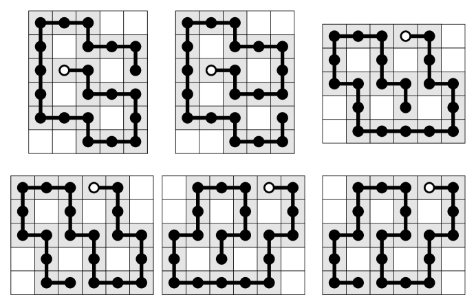
FIG. 2.: The only six conformations of $22$-mer that contain $4$ voids.

FIG. 3.: Geometric properties of chain polymers by exhaustive enumeration. (a) The probability of void formation, (b) the expected number of voids contained in a polymer, (c) the expected void size, and (d) the expected wall size of voids. All these parameters increase with chain length.

FIG. 4.: Voids of fixed size in polymers can have different shapes and thus sometimes different wall sizes. (a) The distribution of the number of observed different wall sizes for a void depends on the size of the void. Voids of size 5 has the maximum number of different wall sizes. (b) The expected wall size for voids of different size in 22-mer.

FIG. 5.: Packing density and compactness are two useful parameters describing packing of chain polymers. (a) The expected packing density decreases with chain length; (b) For 22-mer, the majority of the conformations with 1-void have high packing density, namely, the size of void is small. Fewer conformations are found with large voids. The same pattern is observed for conformations with 2 and 3 voids; (c) The expected compactness fluctuates but in general decreases with chain length; (d) The relationship of average packing density $p$ and average compactness $\rho$ for chain polymer of length $14-22$. Both maximally compact polymer ($\rho=1$) and extended polymer ($\rho=0$) have maximal packing density ($p=1$), but polymers with low packing density have intermediate compactness on average.

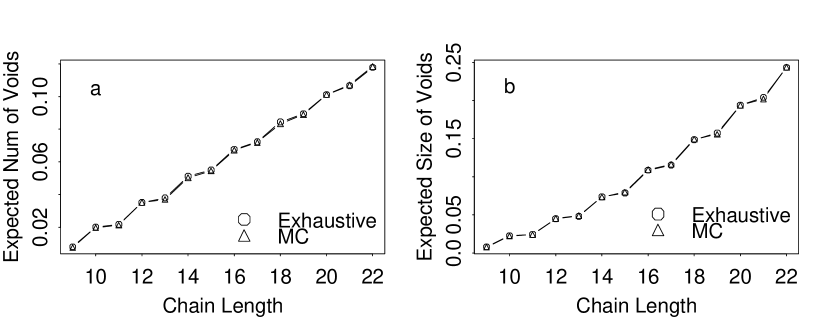
FIG. 6.: Geometric properties obtained by enumeration and by Monte Carlo sampling for polymers of chain length $9-22$. (a) The expected number of voids, and (b) the expected size of voids. Two-step look-ahead sequential Monte Carlo sampling is used, and the sample size is 100,000. These data show that geometric properties estimated by Monte Carlo are identical to those obtained by exhaustive enumeration.

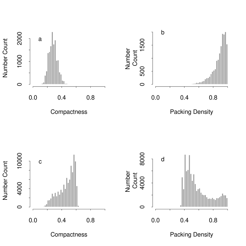
FIG. 7.: The distribution of configurations of polymers obtained by sequential Monte Carlo method can be adjusted by resampling. Sequential Monte Carlo of two step look-ahead without resampling does not generate enough compact conformations. (a) Histogram of conformations at different compactnesses generated without resampling. The compactness of the majority of the conformations is less than 0.5. (b) Histogram of conformations at different packing density generated without resampling. The majority of the conformations are more extended and have higher packing density. The number of conformations with packing density below 0.8 is small. (c) After applying resampling technique favoring compactness of 0.6, the majority of the conformations have compactness between 0.5 and 0.6. Here resampling is applied at each sequential Monte Carlo growth step. (d) Resampling can also be applied to generate conformations with low packing densities with voids. Here resampling favoring low packing density is applied every 2 growth steps. Sample size of 200,000 is used in all calcualtions.

FIG. 8.: Geometric properties of lattice polymers of different lengths, estimated by sequential Monte Carlo method with 2-step look-ahead and resampling technique. Each Monte Carlo simulation starts with a sample size of 200,000. Averaged values of twenty simulations are shown. (a) The probability of void formation increases with chain length. Standard deviation increases slowly with the length. At chain length 200, the standard deviation ($8.5\times 10^{-}3$) is maximum; The expected number of voids (standard deviations $\leq 1.6\times 10^{-}2$) (b) and wall size (standard deviations $\leq 0.25$) (c) are linearly correlated with chain length; (d) The expected void size increases with chain length (standard deviations $\leq 8.3\times 10^{-}3$); (e) The expected packing density decreases with chain length (standard deviations $\leq 7.5\times 10^{-}4$); (f) The expected compactness decreases with chain length and reaches an asymptotic value of $\rho=0.18$ (standard deviations $\leq 5.7\times 10^{-}4$). Different resampling strategies are applied where dead conformations are removed and other conformations with the targeted property is duplicated. Resampling favors conformations with small radius-of-gyration in (a), (b), (c), (d), (e), and conformations with large weight in (f). Resampling is carried out every 5 steps in the process of chain growth.

FIG. 9.: The relationship of expected packing density and compactness for long chain polymer. These data are estimated by sequential Monte Carlo method using 2-step look-ahead and a sample size of $20\times 200,000$ with resampling. Resampling is designed to favor compactness at specified values. The epxected packing density calculated by averaging from the 20 runs has the largest standard deviations for $100$-mer, and are shown in the figure.

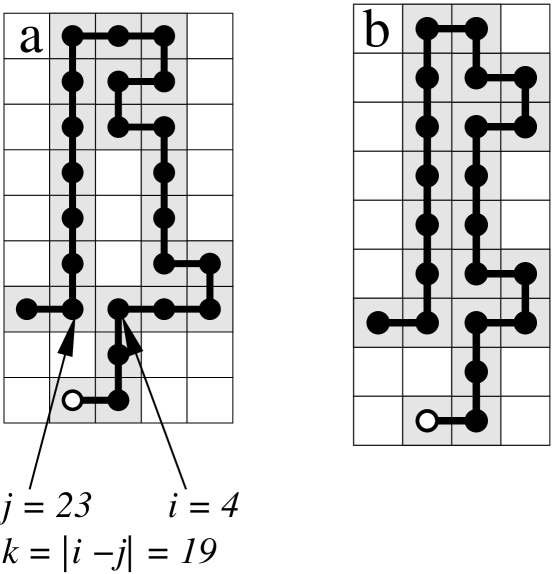
FIG. 10.: The starting position of a void and its wall interval. (a) This 24-mer has a void that starts at $i=4$ and end at $j=23$. Its wall size is $k=19$. (b) This polymer has contact-loop but contains no void.

FIG. 11.: The end-effect of void formation on conformational reduction. (a) Conformational reduction factor $R$ when voids are formed in a 22-chain as examined by enumeration. $R$ depends on the starting position and the wall interval of void; (b) Conformational reduction factor $R$ upto a normalizing constant when voids are formed in a 50-chain as sampled by sequential Monte Carlo (standard deviations $\leq 6.2$). (c) Scaling of conformational reduction factor $R$ and the wall interval $k$ for 50-chain. (standard deviations $\leq 6.4$).

FIG. 12.: Histograms of conformations of 100-mers generated by sequential Monte Carlo with and without resampling at different compactness. In (c) and (d), resampling is applied to every step of the chain growth process. All weighted histogram is normalized so the total area equals to the total number of surviving conformations reaching 100-mer. (a) Histogram of conformations at different compactness generated without resampling. (b) Weighted histogram of conformations generated without resampling, which is proportional to the distribution of all geometrically feasible 100-mers. (c) Histograms of conformations at different compactness when resampling is applied. To resample by weight, dead conformations are replaced with conformations of highest weight. To resample by compactness, dead conformations are replaced with conformations of lowest compactness. Note that the total number of surviving conformations that reach chain length of 100 is much higher then without resampling. Resampling by compactness generates many more conformations with higher compactness. (d) The weighted histograms of conformations under different resampling are in excellent agreement with each other and with that when no resampling is applied.

REFERENCES

- [1] F.M. Richards. Areas, volumes, packing, and protein structures. Ann. Rev. Biophys. Bioeng., 6:151–176, 1977.
- [2] C. Chothia. Structural invariants in protein folding. Nature, 254:304–308, 1975.
- [3] F.M. Richards and W.A. Lim. An analysis of packing in the protein folding problem. Q. Rev. Biophys., 26:423–498, 1994.
- [4] J. Liang and K.A. Dill. Are proteins well-packed? Biophys. J., 81:751–766, 2001.
- [5] B. Lorenz, I. Orgzall, and H-O. Heuer. Universality and cluster structures in continuum models of percolation with two different radius distributions. J. Phys. A: Math. Gen., 26:4711–4722, 1993.
- [6] W.A. Lim and R. Sauer. Alternative packing arrangements in the hydrophobic core of repressor. Nature, 339:31–36, 1989.
- [7] D. Shortle, W.E. Stites, and A.K. Meeker. Contributions of the large hydrophobic amino acids to the stability of staphyloccocal nuclease. Biochemistry, 29:8033–8041, 1990.
- [8] D.D. Axe, N.W. Foster, and A.R. Fersht. Active barnase variants with completely random hydrophobic cores. Proc. Natl. Acad. Sci. USA, 93:5590–5594, 1996.
- [9] R.A. Laskowski, N.M. Luscombe, M.B. Swindells, and J.M. Thornton. Protein clefts in molecular recognition and function. Protein Sci., 5:2438–2452, 1996.
- [10] J. Liang, H. Edelsbrunner, and C. Woodward. Anatomy of protein pockets and cavities: Measurement of binding site geometry and implications for ligand design. Protein Sci, 7:1884–1897, 1998.
- [11] K.F. Lau and K.A. Dill. A lattice statistical mechanics model of the conformational and sequence spaces of proteins. Macromolecule, 93:6737–6743, 1989.
- [12] H.S. Chan and K.A. Dill. Compact polymers. Macromolecules, 22:4559–4573, 1989.
- [13] K.A. Dill. Dominant forces in protein folding. Biochemistry, 29:7133–7155, 1990.
- [14] E. Shakhnovich and A. Gutin. Enumeration of all compact conformations of copolymers with random sequence of links. J. Chem. Phys, 93:5967–5971, 1990.
- [15] C.J. Camacho and D. Thirumalai. Kinetics and thermodynamics of folding in model proteins. Proc. Natl. Acad. Sci. USA, 90:6369–6372, 1993.
- [16] V. S. Pande, C. Joerg, A. Yu Grosberg, and T. Tanaka. Enumeration of the Hamiltonian walks on a cubic sublattic. J. Phys. A, 27:6231, 1994.
- [17] N. D. Socci and J. N. Onuchic. Folding kinetics of proteinlike heteropolymer. J. Chem. Phys., 101:1519–1528, 1994.
- [18] K.A. Dill, S. Bromberg, K. Yue, K.M. Fiebig, D.P. Yee, P.D. Thomas, and H.S. Chan. Principles of protein folding–a perspective from simple exact models. Protein Sci, 4:561–602, 1995.
- [19] A. Šali, E.I. Shakhnovich, and M. Karplus. How does a protein fold? Nature, 369:248–251, 1994.
- [20] I. Shrivastava, S. Vishveshwara, M. Cieplak, A. Maritan, and J. R. Banavar. Lattice model for rapidly folding protein-like heteropolymers. Proc. Natl. Acad. Sci. U.S.A, 92:9206–9209, 1995.
- [21] D.K. Klimov and D. Thirumalai. Criterion that determines the foldability of proteins. Phys. Rev. Lett., 76:4070–4073, 1996.
- [22] R. Mélin, H. Li, N. Wingreen, and C. Tang. Designability, thermodynamic stability, and dynamics in protein folding: a lattice model study. J. Chem. Phys., 110:1252–1262, 1999.
- [23] H.S. Chan and K.A. Dill. The effects of internal constraints on the configurations of chain molecules. J. Chem. Phys., 92:3118–3135, 1990.
- [24] S. Govindarajan and R.A. Goldstein. Searching for foldable protein structures using optimized energy functions. Biopolymers, 36:43–51, 1995.
- [25] H. Li, R. Helling, C. Tang, and N. Wingreen. Emergence of preferred structures in a simple model of protein folding. Science, 273:666–?, 1996.
- [26] M.N. Rosenbluth and A. W. Rosenbluth. Monte Carlo calculation of the average extension of molecular chains. J. Chem. Phys., 23:356–359, 1955.
- [27] D. Frenkel and B. Smit. Understanding molecular simulation: From algorithms to applications. Academic Press, San Diego, 1996.
- [28] D.P. Landau and K. Binder. Monte Carlo simulations in statistical physics. Cambridge University Press, Cambridge, 2000.
- [29] S.W. Golomb. Polyominoes: Puzzles, patterns, problems, and packings. Princeton University Press, 1994.
- [30] F.M. Richards. The interpretation of protein structures: total volume, group volume distributions and packing density. J. Mol. Biol., 82:1–14, 1974.
- [31] H.S. Chan and K.A. Dill. Intrachain loops in polymers: Effects of excluded volume. J. Chem. Phys., 90:492–509, 1989.
- [32] Jun S. Liu. Monte Carlo strategis in scientific computing. Springer, New York, 2001.
- [33] J.S. Liu and R. Chen. Sequential monte carlo methods for dynamic systems. Journal of the American Statistical Association, 93:1032–1044, 1998.
- [34] K.A. Dill. Theory for the folding and stability of globular proteins. Biochemistry, 24:1501, 1985.
- [35] H.S. Chan and K.A. Dill. Energy landscapes and the collapse dynamics of homopolymer. Journal of Chemical Physic, 97:12995–12997, 1993.
- [36] H. Meirovitch. A new method for simulation of real chains: Scanning future steps. J. Phys.A: Math. Gen., 15:L735–L741, 1982.
- [37] J.S. Liu and R. Chen. Blind deconvolution via sequential imputations. Journal of the American Statistical Association, 90:567–576, 1995.
- [38] A. Kong, J.S. Liu, and W.H. Wong. Sequential imputations and Bayesian missing data problems. J. Amer. Statist. Assoc, 89:278–288, 1994.
- [39] J.S. Liu, R. Chen, and W.H. Wong. Rejection control and importance sampling. Journal of American Statistical Association, 93:1022–1031, 1998.
- [40] P. Grassberger. Pruned-enriched Rosenbluth method: Simulation of polymers of chain length up to 1,000,000. Phys. Rev. E., 56:3682–3693, 1997.
- [41] T. Ishinabe and Y. Chikahisa. Exact enumerations of self-avoiding lattice walks with different nearest-neighbor contacts. J. Chem. Phys., 85:1009–1017, 1986.
- [42] T.H. Cormen, C.E. Leiserson, and R.L. Rivest. Introduction to algorithms. The MIT Press, Cambridge, MA, 1990.