Airborne contaminants, e.g., bacterial spores, are usually analyzed by time consuming microscopic, chemical and biological assays. Current research into real time laser spectroscopic detectors of such contaminants is based on e.g. resonance fluorescence. The present approach derives from recent experiments in which atoms and molecules are prepared by one (or more) coherent laser(s) and probed by another set of lasers. These studies have yielded such counterintuitive results as lasers which operate without inversion, ultra-slow light with group velocities of order 10 meters/sec, and generation of ultra-short pulses of light via phased molecular states. The preceding examples are based on inducing a phase coherent state of matter in the ensemble of simple molecules being studied. The connection with previous studies based on “Coherent Anti-Stokes Raman Spectroscopy” (CARS) is to be noted. However generating and utilizing maximally coherent oscillation in macromolecules having an enormous number of degrees of freedom is much more challenging. In particular, the short dephasing times and rapid internal conversion rates are major obstacles. However, adiabatic fast passage techniques and the ability to generate combs of phase coherent femtosecond pulses, provide new tools for the generation and utilization of maximal quantum coherence in large molecules and biopolymers. This extension of the CARS technique is called FAST CARS (Femtosecond Adaptive Spectroscopic Techniques for Coherent Anti-Stokes Raman Spectroscopy), and the present paper proposes and analyses ways in which it could be used to rapidly identify pre-selected molecules in real time.

I Introduction

There is an urgent need for the rapid assay of chemical and biological unknowns, such as bioaerosols. Substantial progress toward this goal has been made over the past decade. Techniques such as fluorescence spectroscopy Cheng ; Seaver99 , and UV resonant Raman spectroscopy Manoharan90 ; Nelson91 ; Ghiamati ; Manoharan93 have been successfully applied to the identification of biopolymers, bacteria, and bioaerosols.

At present field devices are being engineered Seaver99 which will involve an optical preselection stage based on, e.g., fluorescence radiation as in Fig. 1. If the fluorescence measurement does not give the proper signature then that particle is ignored. Most of the time the particle will be an uninteresting dust particle; however, when a signature match is recorded, then the particle is selected for special biological assay, see Fig. 1b. The relatively simple fluorescence stage can very quickly sort out some of the uninteresting particles while the more time consuming bio-tests will only be used for the “suspects”.

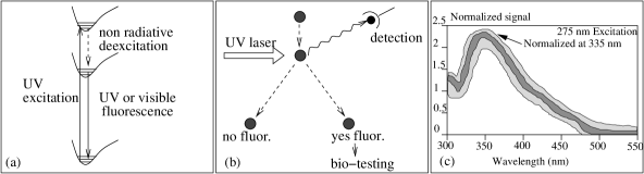
Figure 1: (a) Ultra-violet (UV) excitation radiation promotes molecules from ground state to an excited state manifold. This excited state manifold decays to the ground state via non-radiative processes to a lower manifold which then decays via visible or UV fluorescence. It is this fluorescence signature which is detected in resonance fluorescence spectroscopy; (b) Figure depicting a scenario in which a UV laser interacts with dust particles and bio-spheres of interest. When, for example, a bacterial spore is irradiated, fluorescence will be emitted signaling that this particular system is to be further tested. In principle, uninteresting particles are deflected one way; but when fluorescence takes place, the particles are deflected in another direction and these particles are then subjected to further biological tests; (c) The shaded area displays the signal range for the fluorescence spectrum of a number of biological samples, Bacillus subtilis, Bacillus thuringiensis, Escherichia coli, and Staphylococcus aureus. It is not possible to distinguish between the different samples based on such a measurement (see Cheng for more details).

The good news about the resonance fluorescence technique is that it is fast and simple. The bad news is that while it can tell the difference between dust and bacterial spores, it can not differentiate between spores and many other organic bioaerosols, see Fig. 1c.

However, in spite of the encouraging success of the above mentioned studies, there is still interest in other approaches to, and tools for, the rapid identification of chemical and biological substances. To quote from a recent study Terror :

“Current [fluorescence based] prototypes are a large improvement over earlier stand-off systems, but they cannot yet consistently identify specific organisms because of the similarity of their emission spectra. Advanced signal processing techniques may improve identification.”

Resonant Raman spectra hold promise for being spore specific as indicated in Fig. 2b. This is the good news, the bad news is that the Raman signal is weak and it takes several minutes to collect the data of Fig. 2b. Since the through-put in a set-up such as that of Fig. 1b is large, the optical interrogation per particle must be essentially instantaneous.

The question then is: Can we increase the resonant Raman signal strength and thereby reduce the interrogation time per particle? If so, then the technique may also be useful in various detection scenarios.

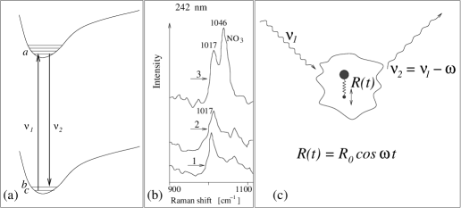
Figure 2: (a) Resonant Raman scattering in which radiation $\nu_{1}$ excites the atom from $|c\rangle$ to $|a\rangle$ and the Stokes radiation is emitted taking the molecule from $|a\rangle$ to $|b\rangle$. The frequency of the excitation radiation is $\nu_{1}$, and the frequency of the Stokes radiation is $\nu_{2}$; (b) Detail of UV resonance Raman spectra of spores of Bacillus megaterium (1), Bacillus cereus (2), and of Calcium Dipicolinate (3), all excited at 242 nm; adapted from W.H. Nelson and J.F. Sperry, Modern Techniques in Rapid Microorganism Analysis, edited by W.H. Nelson (VCH Publishers, N.Y. 1991). Ghiamati (see also Fig. 6); (c) Figure illustrating a more physical picture of Raman scattering in which a single diatomic molecule, consisting of a heavy nucleus e.g. Uranium 235 and a light atom e.g. hydrogen, scattering incident laser radiation at frequency $\nu_{1}$. The vibrational degrees of freedom associated with the diatomic molecule are depicted here as occurring with amplitude $R_{0}$ oscillating at frequency $\omega$. The scattered radiation from this vibrating molecule is at frequency $\nu_{2}=\nu_{1}-\omega$ for the Stokes radiation. This classical picture of the vibrating dipole is to be understood as an amplitude times a sinusoidal oscillation at the frequency $\omega$ as indicated in the equation beneath the figure. $R_{0}$ is a quantum mechanically calculated oscillation amplitude as discussed in detail in Section III of the paper.

The answer to the question of the proceeding paragraph is a qualified “yes.” We can enhance the Raman signal by increasing the coherent molecular oscillation amplitude $R_{0}$ indicated in 2c. In essence this means maximizing the quantum coherence between vibrational states $|b\rangle$ and $|c\rangle$ of 2a.

Our point of view derives from research in the fields of laser physics and quantum optics which have concentrated on the utilization and maximization of quantum coherence. The essence of these studies is the observation that an ensemble of atoms or molecules in a coherent superposition of states represents, in a real sense, a new state of matter aptly called “phaseonium” ScullyZubairy .

In particular, we note that matter in thermodynamic equilibrium has no phase coherence between the electrons in the molecules making up the ensemble. This is discussed in detail in Section III. When a coherent superposition of quantum states is involved, things are very different and based on these observations, many interesting and counterintuitive notions are now a laboratory reality. These include lasing without inversion (LWI) LWI , electromagnetically induced transparency (EIT) EIT , light having ultra slow group velocities on the order of 10 meters/sec slowlight , and the generation of ultra short pulses of light based on phased molecular states sokolov .

Another emerging technology central to the present paper is the exciting progress in the area of femtosecond quantum control of molecular dynamics originally suggested by Judson and Rabitz Rabitz . This is described and reviewed in the articles by Kosloff et al. Kosloff , Warren, Rabitz and Dahleh Warren93 , Gordon and Rice Gordon97 , Zare Zare , Rabitz, de-Vivie-Riedle, Motzkus and Kompa Rabitz00 , and Brixner, Damrauer and Gerber Brixner01 . Other related work on quantum coherent control includes: The quantum interference approach of Brumer and Shapiro Brumer86 ; the time-domain (pump-dump) technique proposed by Tannor, Kosloff and Rice Tannor86 ; the stimulated Raman Adiabatic Passage (STIRAP) approach of Bergmann and co-workers Bergmann98 to generate a train of coherent laser pulses. The preceding studies teach us how to produce pulses having arbitrary controllable amplitude and frequency time dependence. Indeed the ability to sculpt pulses by the femtosecond pulse shaper provides an important new tool for all of optics, see the pioneering works by Heritage, Weiner, and Thurston Heritage , Weiner, Heritage, and Kirschner Weiner88 , Wefers and Nelson Wefers95 and Weiner Weiner00 .

An important aspect of the learning algorithm approach is that knowledge of the molecular potential energy surfaces and matrix elements between surfaces are not needed. Precise taxonomic marker frequencies may not be known a priori; however, by using a pulse shaper coupled with a feedback system, complex spectra can be revealed.

Thus, we now have techniques at hand for controlling trains of phase coherent femtosecond pulses so as to maximize molecular coherence. This allows us to increase the Raman signal while decreasing the undesirable fluorescence background. This has much in common with the CARS spectroscopy Demtroder of Fig. 3, but with essential differences as we now discuss.

The presently envisioned improvement over ordinary CARS is based on enhancing the ground state molecular coherence. However, we note that molecules involving a large number of degrees of freedom will quickly dissipate the molecular coherence amongst these degrees of freedom. This is a well known difficulty and is addressed in the present work from several perspectives. First of all, when working with ultra short pulses, we have the ability to generate the coherence on a time scale which is small compared with the molecular relaxation time. Furthermore, we are able to tailor the pulse sequence in such a way as to mitigate, and overcome key limitations in the application of conventional CARS to trace contaminants. The key point is that we are trying to induce maximal ground state coherence, as opposed to the usual situation within conventional CARS where the ground state coherence is not a maximum as is shown later in this paper. With FAST CARS (Femtosecond Adaptive Spectroscopic Techniques applied to Coherent Anti-Stokes Raman Spectroscopy) we can prepare the coherence between two vibrational states of a molecule with one set of laser pulses; and use higher frequency visible or ultra-violet to probe this coherence in a coherent Raman configuration. This will allow us to capitalize on the fact that maximally coherent Raman spectroscopy is orders of magnitude more sensitive than incoherent Raman spectroscopy.

Figure 3: (a) Ordinary resonant Raman spectroscopy in which a drive laser of amplitude ${\cal E}_{1}$ generates a weak signal field having an amplitude ${\cal E}_{2}$. The incident signal consists of one pulse at $\nu_{1}$ and the pulse structure following interaction with the molecular medium consists of two pulses at $\nu_{1}$ and $\nu_{2}$. (b) The coherent Raman process associated with CARS is depicted in which two fields at frequency ${\nu_{1}}$ and ${\nu_{2}}$ are incident with amplitudes ${\cal E}_{1}$ and ${\cal E}_{2}$. The third radiated anti-Stokes signal field at frequency $\nu_{3}$ is indicated. Hence CARS involves 2 fields in and 3 out. (c) FAST CARS configuration in which maximal coherent Raman spectroscopy is envisioned. The preparation pulses ${\cal E}_{1}$ and ${\cal E}_{2}$ prepare maximum coherence between states $|b\rangle$ and $|c\rangle$. Next the probe laser ${\cal E}_{3}$ interacts with this oscillating molecular configuration and the anti-Stokes radiation is generated. Thus we have 3 fields in and 4 out when using FAST CARS.

Having stated our goals and our approach toward attaining these goals, we emphasize that the present paper represents essentially an engineering endeavor. We propose to draw heavily on the ongoing work in quantum coherence and quantum control as mentioned earlier.

For example, the careful experiments and analysis of the Würzburg group on the generation and probing of ground state coherence in porphyrin molecules Heid01 by femtosecond-CARS (fs-CARS) are very germane to our considerations. However, ground state coherence is not maximized in these experiments.

In another set of beautiful experiments Chen00 they investigate the selective excitation of polymers of diacetylene via fs-CARS. They control the timing, phase and frequency (chirp) content of their preparation pulses. In these experiments it was necessary to focus attention on the evolution of the excited state molecular dynamics. We hope to avoid this complication as is explained later.

Perhaps closest to our approach is the recent joint work of the Garching Max-Planck and Würzburg groups Zeidler02 . Their paper entitled “Optimal control of ground-state dynamics in polymers” is a prime example of a FAST CARS experiment. However they concentrate on producing highly excited states of the “vibrational motion of a certain bond”. The application of their technique to the production of maximum coherence between states $|b\rangle$ and $|c\rangle$ of Fig. 2a in a specific vibrational mode of their molecule would be of great interest to us and is underway.

Finally we wish to draw the reader’s attention to the useful collection of articles in a recent special issue of the “Journal of Raman Spectroscopy” dedicated to fs-CARS JRS00 . Likewise the recent work of Silberberg and coworkers Silberberg in which they show that it is possible to excite one of two nearby Raman levels, even when they are well within the broad fs pulse spectrum is another excellent example of the power of the FAST CARS technique.

To summarize: the present work focuses on utilization of a maximally phase coherent ensemble of molecules, i.e. molecular phaseonium, to enhance Raman signatures. This will be accomplished via the careful tailoring of a coherent pulse designed to prepare the molecule with maximal ground state coherence. Such a pulse is a sort of “melody” designed to prepare a particular molecule. Once we know this molecular melody, we can use it to set that particular molecule in motion and this oscillatory motion is then detected by another pulse; this is the FAST CARS protocol depicted in Figs 3c and 15b.

In order to establish the viability and credibility of this program, the material covered in the present paper is presented in some detail. It is hoped that scientists who are experts in one phase of the subject, e.g., molecular biology but not with subtleties of modern laser spectroscopy can read the paper without undue appeal to the literature or complicated mathematical developments. On the other hand, some basic facts of life, endosporewise, are important. Hence, a short overview of some aspects of Raman spectroscopy as applied to macromolecules and especially to biological spores is presented.

In Section II, the status of Raman spectroscopy applied to biological spores is reviewed. In Section III, we compare various types of Raman spectroscopy with an eye to the recent successful applications of quantum coherence in laser physics and quantum optics. Section IV presents several experimental schemes for applying these considerations to the rapid identification of macromolecules, in general, and biological spores, in particular. Finally in Section V we propose several scenarios in which FAST CARS could be useful in the rapid detection of bacterial spores. Where appropriate, mathematical details are included in Appendices and comparison between the various types of Raman spectroscopic techniques are discussed with special emphasis on overall sensitivity. As stated earlier, the present paper is an engineering science analysis of a promising approach to the problem of bacterial spore detection. This is not a review paper. If the reader feels that we have missed or misrepresented her research, we would be happy to learn how to use it to improve our design and detection strategy. Indeed, we view this paper as providing a point of departure, and will be pleased if it provokes discussion and debate. If the reader is not provoked we apologize. It is very difficult to annoy everybody in a single paper.

II Pico-Review of Raman spectroscopy applied to bacterial spores

The bacterial spore is an amazing life form. Spores thousands of years old have been found to be viable. One textbook Black reports that “endospores trapped in amber for 25 million years germinate when placed in nutrient media.”

A key to this incredible longevity is the presence of dipicolinic acid (DPA) and its salt calcium dipicolinate in the living core which contains the DNA, RNA, and protein as shown in Fig. 4.

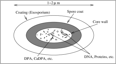
Figure 4: Sketch of spore indicating that the DPA and its salts, e.g., Ca-DPA are contained in the core and are in contact with the spore specific DNA ribosomes and cell proteins.

A major role of the calcium DPA complex seems to be the removal of water, as per the following quote Talaro : “The exact role of these [DNA] chemicals is not yet clear. We know, for instance, that heat destroys cells by inactivating proteins and DNA and that this process requires a certain amount of water. Since the deposition of calcium dipicolinate in the spore removes water . . . it will be less vulnerable to heat.”

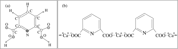
Figure 5: (a) Dipicolinic acid (2, 6-pyridinedicarboxylic acid, C₅H₃N(COOH)₂); (b) The Ca²⁺ DPA complex.

Hence, one of the major components of bacterial spores is dipicolinic acid (DPA) and its ion as depicted in Fig. 5. Calcium dipicolinate can contribute up to $17\%$ of the dry weight of the spores. A definitive demonstration Manoharan90 of this conjecture was made by comparing the 242 nm excitation spectra of calcium dipicolinate with spore suspensions of Bacillus megaterium and Bacillus cereus. From Fig. 6, it is seen that good matches were noted for the 1017, 1396, 1446, and 1607 cm^-1 peaks of the calcium dipicolinate.

As has been emphasized by W. Nelson and coworkers Manoharan90 ; Nelson91 ; Ghiamati ; Manoharan93 , the presence of DPA and its calcium salt gives us a ready made marker for endospores. As has been mentioned earlier and as will be further discussed later, this is the key to Raman fingerprinting of the spore.

We note however that fluorescence spectroscopy was one of the first methods used for detection of bacterial taxonomic markers and is still used for detection where high specificity is not required. This technique is an important addition to the “tool kit” of scientists and engineers working in this area.

Figure 6: This figure (adapted from Nelson91 ) shows UV resonance Raman spectra of spores of Bacillus megaterium (1), spores of Bacillus cereus (2), and calcium dipicolinate (3) in three spectral regions. All samples are excited at 242 nm.

A possible FAST CARS protocol is as follows: First we obtain size and fluorescence information. If this is consistent with the presence of a particular bacterial spore we could then automatically perform a FAST CARS analysis sensitive to DPA so as to further narrow the number of suspects.

It is important to note that just as resonant Raman is some $10^{6}$ times more sensitive than non-resonant, coherent Raman yields a much stronger signal than ordinary incoherent Raman spectroscopy. This makes it possible to collect the Raman spectra much more rapidly via FAST CARS and this is very important in the ultimate scheme of things.

To summarize: we will generate quantum coherence in macromolecules by working with the now available femtosecond pulse trains in which there exists phase coherence between the individual pulses. In this way, one can enhance coherent Raman signatures. The utilization of “molecular music” to generate maximal phase coherence holds promise for the identification and characterization of macro and bio-molecules.

III Comparison of different types of Raman spectroscopy

Raman scattering is an inelastic scattering of electromagnetic fields off vibrating molecules. The origin of Raman scattering dates back to a theoretical paper in Naturwissenschaften by A. Smekal in 1923 entitled (translated) “The quantum theory of dispersion” Smekal . It was followed by another paper in a 1923 Physical Review (by A. Compton) entitled “A quantum theory of the scattering of X-rays by light elements” Compton . Some historians feel that these two papers gave C.V. Raman the idea for the experiments that were performed with K.S. Krishnan and led to the discovery of the effect in over 60 liquids. Raman and Krishnan published their results entitled “A new type of secondary radiation” in Nature on March 28, 1928 Raman . It was soon followed by the landmark paper of G. Landsberg and L. Mandelstam who found the same effect in quartz and published a paper entitled (translated) “A novel effect of light scattering in crystals” which appeared on July 13, 1928 in Naturwissenschaften Landsberg . By the end of 1928 dozens of papers had already been published on the “Raman” effect.

In this section we first recall the quantum mechanical picture of a vibrating molecule. We then discuss the principles of different types of Raman spectroscopy.

III.1 Molecular vibrations

Let us consider a simple diatomic molecule for explanation of the principle. The interatomic oscillation can be visualized via a classical picture of the vibrating molecule as in Fig. 2c. Quantum mechanically, the situation can be understood as depicted in Fig. 7. The potential energy of the molecule depends on the interatomic distance $z$ and has a well pronounced minimum. The Hamiltonian of the vibrating molecule has a set of discrete eigenstates; in Fig. 7 we show just the ground state $|c\rangle$ and the first excited state $|b\rangle$. Whereas in each of these states the mean displacement from the equilibrium position is zero, a quantum superposition of these states has generally a nonzero mean displacement $R(t)$ which varies with time. Assuming that in time $t=0$ the molecule is in a superposition state $|\Psi(0)\rangle=b|b\rangle+c|c\rangle$, then in time $t>0$ the state is $|\Psi(t)\rangle=b|b\rangle+c\exp(-i\omega t)|c\rangle$, where the frequency $\omega=(E_{c}-E_{b})/\hbar$ is the difference of the energies of the eigenstates $|c\rangle$ and $|b\rangle$ divided by the Planck constant $\hbar$. The mean displacement $R(t)$ is then $R(t)=\langle\Psi(t)|\hat{R}|\Psi(t)\rangle$ is then

$$R(t)=R_{0}\exp(\omega t-\varphi_{0})+\text{c.c.},$$ (1)

where

$$R_{0}=\left|bc^{*}\right|\langle b|\hat{R}|c\rangle$$ (2)

is the displacement amplitude, $\varphi_{0}$ is the initial phase (determined by the phases of the coefficients $b$ and $c$), and $\hat{R}$ is the displacement operator. It can be seen from Eq. (2) that one can reach the maximum amplitude of the mean displacement if the superposition coefficients $b$ and $c$ are of the same magnitude, i.e., $|b|=|c|=1/\sqrt{2}$ so that $R_{0}^{\text{max}}=\langle b|\hat{R}|c\rangle/2$. Thus the product $bc^{*}$ is of special importance for determining the vibrational amplitude. This coherent superposition of states is generally described by the off-diagonal density matrix element $\rho_{bc}$ which for the present simple case is given by $\rho_{bc}=bc^{*}$. Without going into detail we simply state that the density matrix element $\rho_{bc}$ is a complex number ($0\leq|\rho_{bc}|\leq 1/2$) characterizing the quantum state of the molecule and determining the amplitude of the mean displacement. For some quantum states quantum coherence is not present (e.g., energy eigenstates, thermal states, etc.), whereas for some states it can reach the maximum magnitude (i.e., for $|\Psi\rangle=2^{-1/2}(|b\rangle+|c\rangle)$).

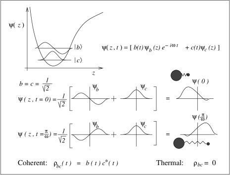
Figure 7: Molecular coherence: atomic distance of a molecule in a coherent superposition of the vibrational states $|b\rangle$ and $|c\rangle$ oscillates periodically with time. On the other hand, a molecule in a thermal equilibrium state is stationary and its coherence $\varrho_{bc}$ vanishes.

We emphasize that when all molecules are in the same superposition state, the response of the sample to an optical signal is very different from the thermal state. Preparation and optical probing of molecular vibrations is the essence of Raman spectroscopy.

III.2 Classical description of the Raman scattering

The simplest classical description of the Raman effect assumes that the polarizability $\alpha$ of the molecule is dependent on the relative positions of the atomic nuclei. The polarizability is the proportionality factor between the external electric field $E$ and the molecular dipole moment $P$, $P=\alpha E$, and for a vibrating molecule it is a time-dependent quantity. In the linear approximation, and assuming just the scalar case, the polarizability can be written as $\alpha(Q)=\alpha(0)+\alpha^{\prime}Q$, where $Q$ is the generalized coordinate of the vibrating molecule, $\alpha(0)$ is the polarizability of the equilibrium state, and $\alpha^{\prime}=\partial\alpha/\partial Q$ with $Q=0$. If the molecule vibrates with frequency $\omega_{bc}$, the coordinate $Q$ changes as $Q=Q_{0}\cos(\omega_{ab}t)$. The electric field irradiating the molecule oscillates as $E=E_{0}\cos(\nu_{1}t)$. Thus, one finds that the molecular dipole oscillates with several frequencies: with the frequency of the incoming radiation $\nu_{1}$ (leading to the Rayleigh scattering), and with the shifted frequencies $\nu_{1}\pm\omega_{bc}$ (leading to the Stokes and anti-Stokes Raman frequencies).

Even though this model is able to predict the correct frequencies of the scattered light, it cannot tell us anything about the intensities of different field components in spontaneous scattering processes. To get more information about the scattering process, one needs a quantum mechanical model of the molecule. Let us now study the main features of the various Raman scattering processes.

III.3 Stokes vs. anti-Stokes scattering

Raman scattering is an optical phenomenon in which there is a change of frequency of the incident light. Light with frequency $\nu_{1}$ scatters inelastically off the vibrating molecules such that the scattered field has frequency $\nu_{2}=\nu_{1}\pm\omega_{bc}$, where $\omega_{bc}$ is the frequency of the molecular vibrations. The field with down-shifted frequency $\nu_{2}=\nu_{1}-\omega_{bc}$ is called Stokes field and its generation corresponds to the process depicted in Fig. 8a, whereas the frequency up-shifted radiation is called the anti-Stokes field and corresponds to the process in Fig. 8b.

Figure 8: Stokes (a) and anti-Stokes (b) Raman scattering. Pump field 1 interacts with a vibrating molecule to produce the scattered field 2 which has either lower frequency (Stokes scattering) or higher frequency (anti-Stokes scattering).

III.4 Spontaneous vs. stimulated Raman scattering

There are two basic Raman processes: the so-called spontaneous and stimulated Raman scattering. Spontaneous scattering occurs if a single laser beam with intensity below a certain threshold illuminates the sample. In condensed matter, in propagating through 1 cm of the scattering medium, only approximately 10^-6 of the incident radiation is typically scattered into the Stokes field (see, e.g., Boyd ). Stimulated scattering which occurs with a very intense illuminating beam is a much stronger process in which several percent of the incident laser beam can be converted into the other frequencies. From the quantum-optical point of view, the Raman scattering can be described by means of photon numbers occupied in different modes. The rate of photon number increase in the Stokes mode can be written as $\dot{n}_{S}=\eta n_{L}(n_{S}+1),$ where $n_{L}$ is the number of photons in the incident laser mode and $n_{S}$ is the number of photons in the Stokes mode. Here $\eta$ is a proportionality constant.

For spontaneous Stokes scattering $n_{S}\ll 1$, and the intensity of the scattered field is roughly proportional to the length traveled by the incident field in the medium. On the other hand, for $n_{S}>1$, the stimulated process becomes dominant and the scattered field intensity can increase exponentially with the medium length.

Process	Raman Coherence $\varrho_{cb}$	Dipole Coherence $\varrho_{ab}~{}\ ~{}$
Raman (Weak drive)	$\displaystyle i\frac{\Omega_{2}\Omega_{1}^{*}}{\gamma_{bc}\Delta}$ $10^{-5}$	(incoh.) $\displaystyle-\frac{\Omega_{2}}{\Delta}\frac{|\Omega_{1}|^{2}}{\Delta\gamma_{bc}}$ $10^{-9}$
Resonant Raman (Weak drive)	$\displaystyle-\frac{\Omega_{2}\Omega_{1}^{*}}{\gamma_{ac}\gamma_{bc}}$    $10^{-2}$	(incoh.) $\displaystyle-\frac{\Omega_{2}}{\gamma_{ab}}\frac{|\Omega_{1}|^{2}}{\gamma_{ac}\gamma_{bc}}$ $10^{-3}$
Raman (Strong drive)	(max. coh.) $\displaystyle\frac{i}{4}\sqrt{\frac{\gamma_{1}}{\gamma_{bc}}}$ $10^{-3}$	(max. coh.)      $\displaystyle i\frac{1}{4}\frac{\Omega_{2}}{\Delta}\sqrt{\frac{\gamma_{1}}{\gamma_{bc}}}$ $10^{-6}$
Resonant Raman (Strong drive)	(max. coh.) $\displaystyle\frac{1}{2}$ $10^{0}$	(max. coh.) $\displaystyle\frac{i\Omega_{1}}{2\gamma_{ab}}$ $10^{-1}$

Table 1: Comparison of different Raman spectroscopic techniques as derived in Appendix A. The density matrix element $\rho_{bc}$ governs the amplitude of coherent vibration, whereas the element $\rho_{ab}$ is proportional to the electronic polarization responsible for emission of radiation. $\Omega_{1,2}$ are the Rabi frequencies, $\Delta$ is the detuning of the electronic transition, $\gamma_{ab}$, $\gamma_{ac}$ are the decay rates of the optical transitions, $\gamma_{bc}$ is the decoherence rate of the vibrational states, and $\gamma_{1}$ is the decay rate from level $b$ to $c$. The approximated values (shown in the lower right corner) were obtained for $\gamma_{ab}\approx\gamma_{ac}\approx\gamma_{bc}\approx 10^{12}$s^-1, $\gamma_{1}\approx 10^{6}$s^-1, $\Delta\approx 10^{15}$s^-1, and $\Omega_{1,2}\approx 10^{11}$s^-1 for weak driving and $\Omega_{1,2}\approx 10^{12}$s^-1 for strong driving. Note that $\Omega\approx 10^{11}$s^-1 corresponds to a 10 ns pulse with 0.1 mJ energy focused on a square millimeter spot if the electronic transition dipole moment is $\wp\approx 10^{-19}$C$\times 10^{-10}$m [see Eq. (A18)].

III.5 Resonant vs. non-resonant Raman processes

The resonant Raman process (appearing when the frequency of the incident radiation coincides with one of the electronic transitions) is much richer than the nonresonant, and we now turn to a discussion of the resonant problem.

Resonant Raman radiation is governed by the oscillating dipole between states $|a\rangle$ and $|b\rangle$ (Stokes) and/or $|a\rangle$ and $|c\rangle$ (anti-Stokes) in the notation of Fig. 3 and Table 1. In the Stokes case, the steady state coherent oscillating dipole $P(t)$, divided by the dipole matrix element $\wp_{ab}=e\langle a|r|b\rangle$, is the important quantity. That is $\rho_{ab}(t)\equiv P(t)/\wp_{ab}$, as given by Eq. (A20), is

$$\varrho_{ab}=-i\left[\Omega_{2}(n_{a}-n_{b})-\Omega_{1}\varrho_{cb}\right]/\left[\gamma_{ab}-i(\omega_{ab}-\nu_{2})\right]$$ (3)

where the Raman coherence is $\rho_{bc}$ as discussed earlier, e.g. Fig. 7. In Eq. (3), $\omega_{ab}$ is the transition frequency between the electronic states $a$ and $b$, $\nu_{2}$ is the frequency of the generated field, and the other quantities are defined in the caption of Table 1.

The main advantage of resonant Raman scattering is that the signal is very strong—up to a million times stronger compared to the signal of nonresonant scattering Nelson91 . It is also very useful that only those Raman lines corresponding to very few vibrational modes associated with strongly absorbing locations of a molecule show this huge intensity enhancement. On the other hand, the resonance Raman spectra may be contaminated with fluorescence. However, this problem can be avoided by using UV light so that most of the fluorescence appears at much longer wavelengths than the Raman scattered light and is easily filtered out.

III.6 Coherent vs. incoherent Raman scattering from many molecules

Figure 9: Incoherent $(a)$ vs. coherent $(b)$ addition of the radiation from $N$ molecules. Each arrow represents the contribution of one molecule to the resulting electric field vector.

An important distinction between different Raman scattering schemes is based on the phase relation of the field scattered off different molecules. In the incoherent case the spontaneous contributions of individual molecules sum up with random phases. The magnitude of the emitted electric field then scales as $\sqrt{N}$ (see Fig. 9a). On the other hand, if all the molecules are prepared in the same coherent superposition of their states $|b\rangle$ and $|c\rangle$, their contributions to the emitted field have the same phases and the magnitude of their sum is proportional to $N$ (see Fig. 9b). Thus, the intensity radiated from the sample is proportional to $N$ in the incoherent case and to $N^{2}$ in the coherent case.

There is another important aspect of the coherent vs. incoherent resonant scattering process, namely the rate of emission from the $N$ atom ensemble. In the far off resonance, Smekel-Raman limit, the emission and absorption are simultaneous since the transitions to the excited state(s) are virtual. This is not true for the resonant Raman processes. In that case the molecule is excited to the $|a\rangle$ state of Fig. 10 where, in the case of weak Stokes field $\varepsilon_{c}$, it can live for many nanoseconds.

Figure 10: (a) Figure depicting resonant Raman experiments at 242 nm in which the molecule is excited to a high lying electronic state while fluorescence occurs at longer wavelengths. (b) By utilizing molecular coherence it is possible to enhance the rate of production of Stokes signal and mitigate fluorescence. (c) Scattering of the high frequency field at $\lambda_{3}$ off surfaces and other states can also be a source of confusion and this is eliminated by using a two photon IR drive.

However, the cooperative emission rate from $N$ molecules can be much faster than that of a single molecule. As was shown by Dicke, and derived in Appendix B, if the spontaneous emission lifetime of $N$ incoherent dipoles is given by $\tau$; then the cooperative spontaneous emission lifetime of $N$ coherently prepared dipoles can be as short as $\tau/N$.

This superradiant “speed up” of the radiation process can have important consequences for the present problem. We recall that the experiments of Nelson and coworkers Manoharan90 ; Nelson91 ; Ghiamati ; Manoharan93 are carried out at 242 nm so as to “ride above” the fluorescence noise, see Fig. 10b. But, if we can enhance the spontaneous emission rate so that the transition rate from the ${a_{2}}$ manifold to the ground state $g$ is faster than from the internal (non radiative) rate from ${a_{2}}\rightarrow{a_{1}}$, it would be possible to mitigate fluorescence noise. Then it would be possible to carry out resonant Raman studies with visible or near UV lasers instead of using the 242 nm wavelength.

IV FAST CARS

IV.1 Generation of atomic coherence

The purpose of this section is to demonstrate the utility of pulse shaping as a mechanism for generating maximal coherence. The Raman signal is optimized at the condition of maximal molecular coherence. When in this state, each of the molecules oscillates at a maximal amplitude, and all molecules in an ensemble oscillate in unison. Here we discuss several methods for the preparation of maximal coherence state.

IV.1.1 Adiabatic Rapid Passage via Chirped Pulses

A particularly simple and robust approach to the generation of the maximal coherence is to use a detuning $\delta\omega$ which is largely independent of inhomogeneous broadening and variations in matrix elements (Fig. 11).

Figure 11: Energy level schematics for a three-level system to generate maximum coherence between the levels $|b\rangle$ and $|c\rangle$ via fields ${\cal E}_{1}$ and ${\cal E}_{2}$. These fields are off-resonant with the electronic detuning $\delta\omega$ and possibly also with the Raman detuning $\Delta\omega$ which can vary in time, thus chirping the pulses. After preparing the coherence $\rho_{bc}$ with fields ${\cal E}_{1,2}$, the probe field ${\cal E}_{3}$ gives rise to the anti-Stokes field ${\cal E}_{4}$.

Such multilevel molecular system can be described in terms of an effective two-by-two Hamiltonian CombGeneration . Diagonalization of this Hamiltonian (Appendix C) allows us to analyze the evolution of the system by drawing analogies to 2-state systems. If the excitation is applied resonantly ($\Delta\omega=0$), such that the initial state of the system (the ground state $|c\rangle$ is projected onto the new basis formed by the eigenvectors $|+\rangle$ and $|-\rangle$ [Eq. (C5)], the system undergoes a sinusoidal Rabi flopping between states $|b\rangle$ and $|c\rangle$. In this situation one can choose to apply a $\pi/2$ pulse in order to create the maximal coherence $|\rho_{bc}|=0.5$.

Alternatively, one can apply an excitation at a finite detuning $\Delta\omega$, to allow all population, which is initially in the ground state, to follow the eigenstate $|+\rangle$ adiabatically. The coherence $\rho_{bc}$ is then

$$\rho_{bc}=\frac{1}{2}\sin\theta\ e^{i\varphi}$$ ()

For molecular systems with large detunings, the Stark shifts $A$ and $D$ are approximately equal and $\theta\cong\tan^{-1}\left(2|B|/2\Delta\omega\right)$, where $B$ is the effective Raman Rabi frequency (Appendix C). One method of achieving the condition $|\rho_{bc}|=0.5$ is to choose $\Delta\omega$ and to increase the product of the two incident fields until $\theta$ is near $90^{\circ}$. This is done adiabatically with the product of the fields changing slowly as compared to the separation of the eigenvalues. Instead, at a fixed field, one may allow $\Delta\omega$ to chirp from an initial value toward zero.

We note that earlier, Grischkowsky Grischkowsky and Oreg et al. Oreg have described preparation mechanisms in two-state and multi-state systems, and Kaplan et al. Kaplan have predicted existence of $2\pi$ Raman solitons.

IV.1.2 Fractional STIRAP

In an all-resonant $\Lambda$ scheme (Fig. 12, with $\delta\omega=\Delta\omega=0$) maximal coherence can be prepared between the levels b and c in a fractional stimulated Raman adiabatic passage (STIRAP) set up by a counterintuitive pulse sequence Bergmann98 ; vss ; Jain , such that the population of the upper state a is always zero and fluorescence from this state is eliminated. This can be accomplished via a counterintuitive sequence of two pulses at frequencies $\omega_{ab}$ and $\omega_{ac}$. Under the condition of adiabatic passage, the molecule in the initial state $|b\rangle$ is transformed into a coherent state $(|b\rangle-|c\rangle)/\sqrt{2}$.

Figure 12: Energy level schematics for the generation of maximum coherence between the levels $|b\rangle$ and $|c\rangle$ via fractional STIRAP by counterintuitive pulses 1 and 2. After a time delay of $\tau$ the pulse resonant with $|{a^{\prime}}\rangle\rightarrow|b\rangle$ transition produces a signal at $\omega_{{a^{\prime}}c}$.

The principle behind a STIRAP process is the adiabatic theorem as applied to the time-varying Hamiltonian $H(t)$. If the system at time $t_{0}$ is in an eigenstate of $H(t_{0})$, and the evolution from $t_{0}$ to $t_{1}$ is sufficiently slow, then the system will evolve into the eigenstate of $H(t_{1})$. The three-level atomic system driven by two fields has three eigenstates, one of which is a linear superposition of only the lower levels $b$ and $c$. The time dependent amplitudes of this eigenstate depend on the pulse shapes of the fields at frequencies $\omega_{ab}$ and $\omega_{ac}$. Thus, by an appropriate pulse shaping, it should be possible to prepare a maximally coherent superposition of states $b$ and $c$ as shown in Fig. 12. The expressions for the Hamiltonian and the corresponding eigenstates are given in Appendix D.

Comparing different schemes for the preparation of maximal coherence, we note that the required laser power is much lower for the all-resonant scheme, but in the case of biomolecules, UV lasers are required. The far-detuned scheme will work with more powerful infrared lasers, up to the point of laser damage. As for the comparison of adiabatic and non-adiabatic regimes, we should note that the adiabatic scheme may turn out to be more robust, because it does not rely on a particular pulse area and works for inhomogeneous molecular ensembles and non-uniform laser beams.

IV.1.3 Femtosecond Pulse Sequences

In a series of beautiful experiments K. Nelson and coworkers KANelson have generated coherent molecular vibration via a train of femtosecond pulses, see Fig. 13. They nicely describe their work as: “Timed sequences of femtosecond pulses have been used to repetitively “push” molecules in an organic crystal…, in a manner closely analogous to the way a child on a swing may be pushed repetitively to reach oscillatory motion.”

An interesting aspect of this approach is the fact that the individual pulses need not be strong. Only the collective effect of many weak pulses is required. This may be helpful if molecular “break-up”, due to strong ${\cal E}_{1}$ and ${\cal E}_{2}$, is a problem. This will be further discussed elsewhere.

Figure 13: Femtosecond pulse train prepares molecular motion, described by $\varrho_{bc}$. The molecular state is then probed by field 3 so that field 4 is produced.

IV.2 Adaptive Evolutionary Algorithms

So far we described how one-photon and two-photon resonant pulse sequences can be used to produce a coherent molecular superposition state. The idea is that once this state is created, a delayed pulse can be applied in order to produce Raman scattering which will bear the signature of the molecular system. The Raman signal is expected to be optimized when the molecular coherence is maximal.

In general, however, things are complicated by the Franck-Condon factors. As an example of a more complicated situation consider Fig. 14. There we see a multilevel system with the ground state $|c\rangle$ and the next state $|c^{\prime}\rangle$. Matrix elements with Franck-Condon overlap factors yield a weak transition between $|c^{\prime}\rangle$ and $|a\rangle$ or $|a^{\prime}\rangle$ as indicated in the figure. However, given an appropriately nonlinear ground state potential it is quite possible that the next vibrational state could be off-set and have the appropriate position of the peaks of the wave function in order to maximize the Franck-Condon overlap. In this way, the coherence between the states $|b\rangle$ and $|c\rangle$ of Fig. 14 could still serve as a strong generator of the anti-Stokes radiation on the $|a\rangle$ to $|b\rangle$ transitions.

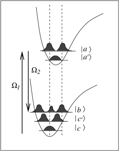
Figure 14: Schematics to generate coherence between the levels $|b\rangle$ and $|c\rangle$. The shaded curves represent the probability distribution of the interatomic distance for different vibrational and electronic states.

Given such a configuration, it is not hard to see how to prepare the ground state coherence. We could, for example, radiate the molecule with a chirped Raman pair so as to generate maximal coherence between $|b\rangle$ and $|c^{\prime}\rangle$ and then follow that by a Raman $\pi-$pulse transferring the population from $|c^{\prime}\rangle$ to $|c\rangle$. In this way, maximal coherence between $|c\rangle$ and $|b\rangle$ would be prepared. And as indicated in the figure, strong matrix elements would be expected between $|b\rangle,|c\rangle$ and the first excited vibrational state of the electronic potential.

The preceding example shows that even in a simplified ideal few-level system, preparation of maximal molecular coherence may require application of a complicated pulse sequence. For large bio-molecules the level structure is not only much more complex, but usually unknown. We now consider how search algorithms can be used to find the optimal pulse sequence for a complicated molecule with an unknown Hamiltonian. This approach will eventually lead to an efficient generation of “molecular fingerprints”.

In order to achieve this goal we will need to (1) utilize a technique for preparation of complex shaped pulse sequences; (2) find the particular pulse sequences, required for the excitation of the particular bio-molecules and for the production of spectral signatures, which will allow one to distinguish (with certainty) the target biological agent from any other species.

Pulse shaping techniques already exist; they are based on “spectral modification”. First, a large coherent bandwidth is produced by an ultra-short pulse generation technique Krausz . Then, the spectrum is dispersed with a grating or a prism, and each frequency component is addressed individually by a spatial light modulator (a liquid crystal array Weiner or an acoustic modulator Warren ). This way, individual spectral amplitudes and phases can be adjusted independently. Finally, the spectrum is recombined into a single beam by a second dispersive element, and focused onto the target. This technique allows synthesis of arbitrarily shaped pulses right at the target point, and avoids problems associated with dispersion of intermediate optical elements and windows.

A particular shaped pulse sequence can be represented by a three-dimensional surface in a space with frequency-amplitude-phase axes. Each pulse shape, which corresponds to a particular 3-D surface, produces a molecular response. The problem is to find the optimal shape. The search space is too large to be scanned completely. Besides, many local optima may exist in the problem. The solution is offered by “global search” algorithms (such as adaptive evolutionary algorithms) Assion ; Gerber . In this approach the experimental output is included in the optimization process. This way, the molecules subjected to control, are called upon to guide the search for an optimal pulse sequence within a learning loop Rabitz . With the proper algorithm, automated cycling of this loop provides a means of finding optimal pulse shapes under constraints of the molecular Hamiltonian and the experimental conditions. No prior knowledge of the molecular Hamiltonian and the potential energy surfaces is needed in this case.

This adaptive technique was developed for coherent control of chemical reactions Gerber . The idea is that the pulses can be optimized to produce desired chemical products. In our problem we want to optimize Raman generation. In this case both preparation and reading pulses can be adaptively shaped in order to maximize the signal. Fig. 15 shows schematics for the experimental setup that implements these ideas.

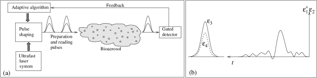
Figure 15: (a) Experimental setup for the implementation of adaptive techniques; (b) Figure depicting amplitude of possible optimized Raman preparation pulse sequence ${\cal E}^{*}_{1}{\cal E}_{2}$. Not indicated is the fact that the “reading” pulse ${\cal E}_{3}$ can also be profitably considered as a learning algorithm variable.

Generated spectra will be different for different molecular species. And our task is not only to maximize Raman generation, but also to identify spectral patterns characteristic of particular species and maximize the difference in the spectrum produced by the target bio-molecule from spectra produced by any other bio-molecules. The key idea here is to apply the same adaptive algorithms in order to learn these optimal “molecular fingerprints”.

We note that the complexity of the molecular level structure is not so much a problem as a solution to a problem. We can take advantage of the richness of the molecular structure, and the infinite variety of possible pulse shapes, in order to distinguish different species with the required certainty.

V Possible FAST CARS measurement strategies for detection of bacterial spores

Having presented the FAST CARS technique in some detail we now return to the question of its application to “fingerprinting” of macromolecules and bacterial spores. Some aspects of the technique seem fairly simple to implement and would seem to hold relatively immediate promise. Others are more challenging but will probably be useful at least in some cases. Still other applications, e.g., the stand-off detection of bioaerosols in the atmosphere present many open questions and require careful study. In the following we discuss some simple FAST CARS experiments which are underway and/or being assembled in our laboratories.

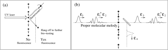
Figure 16: (a) Two-stage detection scheme. Airborne particles are irradiated with a UV laser. Those particles which fluoresce are selected for further testing. (b) FAST CARS testing of the preselected particles is like “singing a song” and listening for the standing ovation after an intricate aria. That is, the signal is generated only when a particular molecule hears its molecular melody.

V.1 Preselection and hand-off scenarios

At present, field devices are being engineered which will involve an optical preselection stage based on, e.g., fluorescence tagging. If the fluorescence measurement does not match the class of particles of interest then that particle is ignored. When many such particles are tested and a possible positive is recorded, the particle is subjected to special biological assay; see Fig. 16a. Such a two stage approach can substantially speed up the detection procedure. The relatively simple fluorescence stage can very quickly sort out many uninteresting scattering centers while the more sophisticated Raman scattering protocol will only be used for the captured “suspects”.

The properly shaped preparation pulse sequence will be determined by, e.g., the adaptive learning algorithm approach as per section IV.2. The amplitude and phase content of the pulse which produces maximum oscillation may be linked to a musical tune. Each spore will have a song which results in maximum Raman coherence. A correctly chosen “melody” induces a characteristic response of the molecular vibrations—a response which is as unique as possible for the bacterial spores to be detected. Playing a melody rather than a single tone is a generalization that enables us to see a multidimensional picture of the investigated object. We note that the optimization can (and frequently will) include not only the preparation pulses 1 and 2 (see Fig. 15b), but also the probe pulse 3, in particular, its central frequency and timing. Analysis of the response to such a complex input is a complicated signal processing problem. Various data mining strategies may be utilized in a way similar to speech analysis.

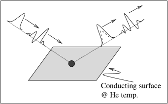
Figure 17: Surface Raman payoff: Proof of principle we are carrying out, utilizing a cold (He⁴ temperature) sample so as to enhance the Raman signatures and minimize $\gamma_{bc}$.

However, taking into account the fact that we work with femtosecond pulses chained in picosecond to nanosecond pulse trains, the whole analysis can be very short. In particular, if we recall the long sampling time of the complete fluorescence spectra of Ghiamati being $\approx 15$min, our estimation of a microsecond analysis is a very strong argument for the chosen approach.

V.2 Possible further Raman characterization

After a suspect particle has been targeted, it may be subject to a whole variety of investigative strategies. Raman scattering off a flying particle can be very fast, but not necessarily the most accurate method. It will be very useful to pin the particle on a fixed surface and cool it down to maximize the decoherence time $T_{2}$ so that the characteristic lines are narrowed down. The particle can be deflected by optical means (laser tweezers, laser ionization, etc.) and attached to a cooled conducting surface (see Fig. 17). Cooling to liquid helium temperature would enable us to enhance the dephasing time from $T_{2}\sim 10^{-12}$sec at room temperature to $T_{2}\lesssim 10^{-9}$sec at a few degrees Kelvin.

V.3 Possible spore specific FAST CARS detection schemes

We conclude with some speculative observations for long range (stand-off) measurements.

Figure 18: Influence of various radicals on the frequency of the symmetric NO₂ vibrations.

The chemical state of DPA in the spore is of special interest to us because the stuff we hang on the DPA molecule will determine its characteristic Raman frequency. To this end, we quote from article Murrell by Murrell on the chemical composition of spores: “When DPA is isolated from spores it is nearly always in the Ca-CDPA chelate but sometimes as the chelate of other divalent metals [e.g. Zn, Mn, Sr etc.] and perhaps as a DPA-Ca amino complex.”

Thus, since each different type of spore would have its own unique mixture of metals and amino acids, it may be the case that the finer details of the Raman spectra would contain spore specific “fingerprints.” This conjecture is supported by Fig. 2b where the difference between the DPA Raman spectra of the spores of Bacillus cereus and Bacillus megaterium is encouraging.

The open question is: to what extent is the DPA Raman spectra sensitive to its environment? That we might be able to achieve spore specific sensitivity is consistent with the well known fact that substituents, e.g., NO₂ experience a substantial shift of their vibrational frequencies when bound in different molecular configurations, see Fig. 18. Furthermore, recent NMR experiments Leuschner01 show spore specific fingerprints due to the local environment (see Fig. 19).

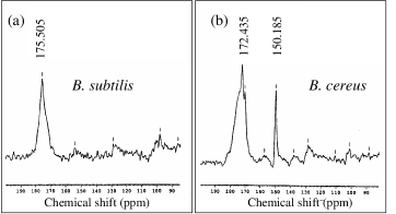
Figure 19: Nuclear magnetic resonance ¹³C Cross polarization magic angle spinning (CPMAS) spectrum of (a) outer coatless mutant Bacillus subtilis 322 spores and (b) dormant Bacillus cereus spores. Complete spectra is found in Leuschner01 .

Clearly there are many oportunities and open questions implicit in the FAST CARS “molecular melody” approach to real time spectroscopy. However it plays out, this combination of quantum coherence and coherent control promises to be a fascinating area of research.

Appendix A Three level system driven by two fields

In this appendix we consider the density matrix approach to the Raman scattering and discuss various limiting cases. In particular we present a semiclassical treatment in which the field evolution is described by Maxwell’s equations and the atomic system by the density operator.

We consider a three level atomic system in the $\Lambda$ configuration with upper level a and lower levels b and c. The $a\rightarrow b$ transition is driven by a field at frequency $\nu_{1}$ and the $a\rightarrow c$ transition is coupled via a signal field at frequency $\nu_{2}$.

The Maxwell’s equations lead to the following equation for the evolution of the signal field,

$$\left(\frac{\partial^{2}}{\partial z^{2}}-\frac{1}{c^{2}}\frac{\partial^{2}}{\partial t^{2}}\right)E = \mu_{o}\ddot{P},$$ (A1)

where $E$ is the electric field vector of the emitted light, $\mu_{o}$ is the vacuum permeability, and P is the medium polarization. We write the electric field using the slowly varying envelope E as

$$E = \frac{1}{2}{\cal E}(z,t)e^{-i(\nu t-kz+\phi)}+c.c.$$ (A2)

and write the polarization in terms of the slowly varying quantity $P$ as

$$P = \frac{1}{2}{\cal P}(z,t)e^{-i(\nu t-kz+\phi)}+c.c.\ .$$ (A3)

Working within the slowly varying amplitude and phase approximation, Eqs. (A1), (A2), and (A3) yield

$$\frac{1}{c}\frac{\partial{\cal E}}{\partial t}+\frac{\partial{\cal E}}{\partial z}=-\frac{1}{2\epsilon_{0}}k\text{Im}{\cal P},$$ (A4)

where

$${\cal P}=2{\cal N}(z,t)\wp_{ab}\varrho_{ab}e^{i(\nu t-kz+\phi)}.$$ (A5)

Here $\wp_{ab}$ is the dipole moment matrix element, $\varrho_{ab}$ is the off-diagonal element of the density matrix for the molecular levels $a$ and $b$, and ${\cal N}(z,t)$ is the volume density of the molecules. We note that the electromagnetic field is determined by $\varrho_{ab}$.

Figure 20: Schematic diagram of the Raman interaction for the three-state system. The driving fields 1 and 2 are in Raman resonance with the two lower levels $b$ and $c$, but are generally off-resonant with the transitions to the excited state $a$ (with detuning $\Delta$). Decoherence and decay of the optical transitions $ab$ and $ac$ are characterized by the rates $\gamma_{ab}$ and $\gamma_{ac}$, the spontaneous decay rate of level $b$ to $c$ is $\gamma_{1}$, and the decoherence rate of the $bc$ transition is $\gamma_{bc}$.

Here we recall the main results of Dream and apply them to our physical situation (see Fig. 20). First we define the decay rates

$$\gamma_{ab} = \frac{\gamma+\gamma_{1}}{2}+\gamma_{ab}^{p},$$ (A6)

$$\gamma_{ca} = \frac{\gamma}{2}+\gamma_{ca}^{p},$$ (A7)

$$\gamma_{cb} = \frac{\gamma_{1}}{2}+\gamma_{cb}^{p}.$$ (A8)

Here the decay rates from $a$ to $b$ is $\gamma_{b}$, and from $a$ to $c$ is $\gamma_{c}$, and $\gamma=\gamma_{b}+\gamma_{c}$. Population decay rate from $b$ to $c$ is $\gamma_{1}$. Purely phase decays are designated by the superscript $p$. Complex dephasings are defined as

$$\Gamma_{ab} = \gamma_{ab}-i\Delta_{ab},$$ (A9)

$$\Gamma_{ca} = \gamma_{ca}+i\Delta_{ac},$$ (A10)

$$\Gamma_{cb} = \gamma_{cb},$$ (A11)

where $\Delta_{ac}=\omega_{ac}-\nu_{1}$ and $\Delta_{ab}=\nu_{2}-\omega_{ab}$. In the following we assume Raman resonance, i.e., $\Delta_{ac}=-\Delta_{ab}=\Delta$. The main working equations for the off-diagonal density matrix elements are

$$\dot{\varrho}_{ab} = -\Gamma_{ab}\varrho_{ab}+i\Omega_{2}(\varrho_{bb}-\varrho_{aa})+i\Omega_{1}\varrho_{cb},$$ (A12)

$$\dot{\varrho}_{ca} = -\Gamma_{ca}\varrho_{ca}+i\Omega_{1}^{*}(\varrho_{aa}-\varrho_{cc})-i\Omega_{2}^{*}\varrho_{cb},$$ (A13)

$$\dot{\varrho}_{cb} = -\Gamma_{cb}\varrho_{cb}-i\Omega_{2}\varrho_{ca}+i\Omega_{1}^{*}\varrho_{ab}.$$ (A14)

The equations for the populations are

$$\dot{\varrho}_{bb} = i\Omega^{*}_{2}\varrho_{ab}-i\Omega_{2}\varrho_{ba}+\gamma_{b}\varrho_{aa}-\gamma_{1}\varrho_{bb},$$ (A15)

$$\dot{\varrho}_{cc} = i\Omega^{*}_{1}\varrho_{ac}-i\Omega_{1}\varrho_{ca}+\gamma_{c}\varrho_{aa}+\gamma_{1}\varrho_{bb},$$ (A16)

and $\varrho_{aa}$ is obtained from

$$1 = \varrho_{aa}+\varrho_{bb}+\varrho_{cc}.$$ (A17)

Here $\Omega_{1,2}$ are the Rabi frequencies of the fields having frequencies $\nu_{1,2}$, i.e.,

$$\Omega_{1} = \frac{\wp_{ac}{\cal E}_{1}}{\hbar},$$ (A18)

$$\Omega_{2} = \frac{\wp_{ab}{\cal E}_{2}}{\hbar},$$ (A19)

The steady state solution of these equations can be obtained by setting all time derivatives equal to zero. The result is

$$\framebox{$\displaystyle\varrho_{ab}=-\frac{i}{\Gamma_{ab}}[\Omega_{2}(\varrho_{aa}-\varrho_{bb})-\Omega_{1}\varrho_{cb}],$}$$ (A20)

and

$$\varrho_{ca} = \frac{i\Omega_{1}^{*}}{\cal D}\left[(\varrho_{aa}-\varrho_{cc})(\Gamma_{ab}\Gamma_{cb}+|\Omega_{1}|^{2})+(\varrho_{bb}-\varrho_{aa})|\Omega_{2}|^{2}\right],$$ (A21)

$$\varrho_{cb} = \frac{\Omega_{2}\Omega_{1}^{*}}{\cal D}\left[(\varrho_{aa}-\varrho_{bb})\Gamma_{ca}+(\varrho_{aa}-\varrho_{cc})\Gamma_{ab}\right],$$ (A22)

where the common denominator is

$${\cal D}=\Gamma_{ab}\Gamma_{ca}\Gamma_{cb}+\Gamma_{ab}|\Omega_{2}|^{2}+\Gamma_{ca}|\Omega_{1}|^{2}.$$ (A23)

Equation (A20) is our main working equation. The first term in the parenthesis of Eq. (A20) is responsible for the stimulated emission or absorption on the $|a\rangle\leftrightarrow|b\rangle$ transition. The second, $\varrho_{cb}$, term describes the Raman conversion of $\nu_{1}$ into $\nu_{2}$. As we can see, it is crucial to have the element $\varrho_{cb}$ as big as possible for optimum Raman conversion. In the following we present the main properties of $\varrho_{cb}$ for various experimental and conceptual configurations and consider various limiting cases for the Raman processes.

A.1 Off-resonant Raman process, weak driving

First we consider the Raman effect far from electronic resonance ($\Delta\gg\gamma_{ab},\gamma_{ac}$). In this case the upper level $a$ is almost completely depopulated and can be eliminated from the dynamics. The system behaves basically as a two-level system with the Rabi frequency of oscillations between levels $b$ and $c$ equal to $\Omega_{R}=|\Omega_{1}^{*}\Omega_{2}|/\Delta$. For dephasing rate $\gamma_{bc}\gg\Omega_{R}$, we find the steady state solution for the lower state coherence $\varrho_{cb}$ as

$$\lim_{\Delta\gg\gamma}\varrho_{cb} = \hskip 7.11317pti\frac{\Omega^{*}_{1}\Omega_{2}}{\gamma_{bc}\Delta}(\varrho_{cc}-\varrho_{bb}),$$ (A24)

which, after substituting into Eq. (A20), yields the density matrix element responsible for the $\nu_{2}$ radiation as

$$\varrho_{ab}^{\text{Raman}} = -i\frac{\Omega_{2}}{\gamma_{ab}-i\Delta}\left[(\varrho_{aa}-\varrho_{bb})-i\frac{|\Omega_{1}|^{2}}{\gamma_{bc}\Delta}(\varrho_{cc}-\varrho_{bb})\right].$$ (A25)

Note that for the amplification of the $\nu_{2}$ field the so-called Raman inversion $\varrho_{cc}-\varrho_{bb}$ is necessary. In the simplest case when almost all the molecules are in the lowest state $c$, $\varrho_{cc}\approx 1$, $\varrho_{bb}\approx 0$, $\varrho_{aa}\approx 0$, Eq. (A25) reduces to

$$\varrho_{ab}^{\text{Raman}} = -i\frac{\Omega_{2}}{\Delta}\frac{|\Omega_{1}|^{2}}{\Delta\gamma_{bc}}.$$ (A26)

A.2 Off-resonant Raman process, strong driving

In the case of strong driving the transition between states $b$ and $c$ can be saturated so that both these levels are significantly populated (with virtually no population in the excited state $a$). In particular, one obtains from Eq. (A15) the steady state populations of the lower levels

$$\rho_{bb}=\frac{i\Omega_{2}^{*}\rho_{ab}-i\Omega_{2}\rho_{ba}}{\gamma_{1}},$$ (A27)

and $\rho_{cc}=1-\rho_{bb}$. Substituting Eq. (A20) into Eq. (A27), and assuming, without loss of generality, that the Rabi frequencies for the laser fields are real ($\Omega_{1}=\Omega_{1}^{\ast},\Omega_{2}=\Omega_{2}^{\ast}$) we find that for the far off-resonant case ($\Gamma_{ab}\approx i\Delta$)

$$\rho_{bb}=\frac{2\Omega_{2}\Omega_{1}\rho_{bc}}{i\Delta\gamma_{1}}.$$ (A28)

Rearranging Eq. (A22) and inserting Eq. (A28), under the condition

$$\gamma_{bc}\gg\left|-\frac{|\Omega_{1}|^{2}}{i\Delta}+\frac{|\Omega_{2}|^{2}}{i\Delta}\right|,$$ (A29)

we find that

$$\rho_{bc}=-\frac{\Omega_{2}\Omega_{1}}{i\Delta\Gamma_{bc}}-\frac{4\Omega_{2}^{2}\Omega_{1}^{2}\rho_{bc}}{\gamma_{1}\Delta^{2}\Gamma_{bc}}.$$ (A30)

Solving Eq. (A30) for $\rho_{bc}$ we obtain

$$\rho_{bc}=\frac{i\Omega_{2}\Omega_{1}}{\Delta}\left(\gamma_{bc}+\frac{4\Omega_{2}^{2}\Omega_{1}^{2}}{\gamma_{1}\Delta^{2}}\right)^{-1}.$$ (A31)

It can be shown that the maximum magnitude of the coherence $|\rho_{bc}|$ is given by

$$\left|\rho_{bc}\right|=\sqrt{\frac{\gamma_{1}}{16\gamma_{bc}}}.$$ (A32)

This maximum occurs when

$$\frac{\Omega_{1}\Omega_{2}}{\Delta}=\frac{\sqrt{\gamma_{1}\gamma_{bc}}}{2}.$$ (A33)

A.3 Resonant Raman process, weak driving

In the resonant case ($\Delta=0$), the Raman effect has much in common with the scheme of lasing without inversion (LWI; see, e.g., Dream ). The lower state coherence is then found to be

$$\varrho_{cb}\stackrel{{\scriptstyle\Delta=0}}{{\longrightarrow}}\hskip 7.11317pt\Omega_{2}\Omega^{*}_{1}\frac{[(\varrho_{aa}-\varrho_{bb})\gamma_{ca}+(\varrho_{aa}-\varrho_{cc})\gamma_{ab}]}{\gamma_{ab}\gamma_{ac}\gamma_{cb}+\gamma_{ca}|\Omega_{1}|^{2}+\gamma_{ab}|\Omega_{2}|^{2}}.$$ (A34)

Polarization responsible for the $\nu_{2}$ radiation is then governed by

$$\varrho_{ab}=-i\frac{\Omega_{2}}{\gamma_{ab}}\left[(\varrho_{aa}-\varrho_{bb})\left(1-\frac{|\Omega_{1}|^{2}\gamma_{ca}}{D}\right)-(\varrho_{aa}-\varrho_{cc})\frac{|\Omega_{1}|^{2}\gamma_{ab}}{D}\right],$$ (A35)

where $D=\gamma_{ab}\gamma_{ca}\gamma_{cb}+\gamma_{ab}|\Omega_{2}|^{2}+\gamma_{ca}|\Omega_{1}|^{2}$.

In the weak driving limit ($\Omega_{1,2}\ll\gamma_{ab},\gamma_{ac},\gamma_{bc}$), almost all the population remains in state $c$ ($\varrho_{cc}\approx 1$, $\varrho_{bb}\approx 0$, $\varrho_{aa}\approx 0$). The atomic coherence of the lower levels is

$$\rho_{cb}=-\frac{\Omega_{1}^{*}\Omega_{2}}{\gamma_{ac}\gamma_{bc}},$$ (A36)

and the corresponding expression for the density matrix element $\rho_{ab}$ is

$$\varrho_{ab}^{\text{Resonant Raman}}=-i\frac{\Omega_{2}}{\gamma_{ab}}\frac{|\Omega_{1}|^{2}}{\gamma_{ac}\gamma_{bc}}.$$ (A37)

A.4 Resonant Raman process, strong driving

In the resonant case we can find the steady state solution of a strongly driven three-level system ($|\Omega_{1,2}|\gg\gamma_{1},\gamma_{bc}$) in the form of the so-called dark state. It is useful to consider two superpositions of the lower states $|b\rangle$ and $|c\rangle$ defined as

$$|B\rangle = \frac{\Omega_{2}|b\rangle+\Omega_{1}|c\rangle}{\Omega},$$ (A38)

$$|D\rangle = \frac{\Omega_{1}|b\rangle-\Omega_{2}|c\rangle}{\Omega},$$ (A39)

where $\Omega=\sqrt{|\Omega_{1}|^{2}+|\Omega_{2}|^{2}}$. The state $|D\rangle$ is completely decoupled from the upper state $|a\rangle$ ($\hat{H}|D\rangle=0$), and is called the dark state. If the molecule starts in any state different from $|D\rangle$, the fields $\Omega_{1}$ and $\Omega_{2}$ will promote it to the upper state $|a\rangle$, which decays to the lower states by spontaneous emission. If the molecule is in $|D\rangle$ it stays there unchanged. In this way the dark component of the state increases and finally the system will end up completely in the state $|D\rangle$. The populations of the levels $a$ and $b$ are $\rho_{aa}=0$ and $\rho_{bb}=|\Omega_{1}|^{2}/\Omega^{2}$, and the dark state coherence of the lower states is, as given by Eq. (A39),

$$\varrho_{cb} = -\frac{\Omega^{*}_{1}\Omega_{2}}{\Omega^{2}}.$$ (A40)

Maximum Raman coherence is achieved with $|\Omega_{1}|=|\Omega_{2}|$ so that $|\rho_{bc}^{\text{max}}|=1/2$. The element $\varrho_{ab}$ [see Eq. (A20)] responsible for the radiation is given by

$$\varrho^{\text{Dark Raman}}_{ab} = -\frac{i}{\gamma_{ab}}\left[\Omega_{2}(\varrho_{aa}-\varrho_{bb})+\frac{|\Omega_{1}|^{2}\Omega_{2}}{\Omega^{2}}\right]=0,$$ (A41)

i.e., there is no radiation from the dark state. To obtain Raman signal one can, e.g, switch off the field $\Omega_{2}$ after reaching the maximum coherence $|\varrho_{cb}^{\text{max}}|=1/2$. Then the density matrix element $\varrho_{ab}$ goes as

$$\varrho_{ab}^{\text{Max coherence}}=i\frac{\Omega_{1}}{2\gamma_{ab}}.$$ (A42)

To summarize the main results of this appendix, we display the density matrix elements responsible for the signal field generation in Table 1.

Appendix B Cooperative Spontaneous Emission

Since the DPA is contained in the small ($V\sim(1\mu)^{3}$) volume of the core and since the number of participating DPA molecules is huge ($N\gtrsim 10^{9}$) the possibility of Dicke superradiance should be carefully considered. At the outset, we should note that the short dephasing times of vibronic levels ($T_{2}$ is in the picosecond range) and the unknown inhomogeneous dephasing time $T_{2}^{\ast}$ will tend to wash out the effect. Still, if the spontaneous emission time ($\tau\sim 1-10$ nanoseconds) is reduced by even a small fraction of N, then cooperative spontaneous emission may be important.

Motivated by the proceeding we now turn to a short review of the effect from the present, FAST CARS, perspective. We focus on two levels $|a\rangle$ and $|b\rangle$. The previous pulses $\varepsilon_{1}$ and $\varepsilon_{2}$ beat the coherence between $|b\rangle$ and $|c\rangle$ so that at time $t=0$

$$|\Psi(0)\rangle=B|b\rangle+C|c\rangle,$$ (B1)

the third pulse, arriving at time T, promotes $|c\rangle\rightarrow|a\rangle$ so that at time $t=\tau$

$$|\Psi(\tau)\rangle=A|a\rangle+B|b\rangle+C^{\prime}|c\rangle.$$ (B2)

Hence the atoms at time $\tau$ are in a coherent superposition $|a\rangle$ and $|b\rangle$ and this affects the rate of spontaneous emission from the N molecules involved.

For the present purposes it is best to start with the Hamiltonian describing the interaction of N two level systems ($|a\rangle$ and $|b\rangle$) and the quantized radiation field given by

$$H_{\text{int}}=\Sigma_{i,k}\hbar ga^{+}_{k}\sigma_{i}e^{ik\cdot r_{i}}+adj$$ (B3)

where, as discussed, e.g., in ScullyZubairy , $g_{k}$ is the coupling frequency between the molecules and the $k^{th}$ mode of the field, $a^{+}_{k}$ is the usual creation operator and $\sigma_{i}=(|b\rangle\langle a|)_{i}$ is the lowering operator for the $i^{th}$ molecule.

Consider next the case in which all molecules are located at $r_{i}=r_{0}$ in a volume small compared to the radiation wavelength $\lambda$, and noting that the coupling constant is a slowly varying function of $k$ we may write

$$H_{\text{int}}=\left[g_{k}e^{ik_{0}\cdot r_{0}}\sum_{k}a^{+}_{k}\right]\sum_{i}\sigma_{i},$$ (B4)

The important point being that the lowering operator described by Eq. (B4) is symmetric in the molecular lowering operator $\sigma_{i}$.

To glean the physics from Eq. (B4) it is enough to consider 3 molecules which are all started in their upper state, so that

$$|\Psi_{3}\rangle=|a_{1}a_{2}a_{3}\rangle.$$ (B5)

The state (B5) evolves under the influence of the field according to the interaction (B4), and the molecular state develops into $|\Psi_{3}\rangle\rightarrow\alpha|\Psi_{3}\rangle+\beta|\Psi_{2}\rangle$ where $\alpha$ and $\beta$ are uninteresting constants and

$$|\Psi_{2}\rangle=\sum_{i}\sigma_{i}|\Psi_{3}\rangle=|b_{1}a_{2}a_{3}\rangle+|a_{1}b_{2}a_{3}\rangle+|a_{1}a_{2}b_{3}\rangle.$$ (B6)

In general the symmetric interaction (B4) only couples the $|a_{1}a_{2}a_{3}\rangle$ state to the symmetric states of Fig. 21.

Figure 21: Showing that the symmetric combinations of the molecular states $|a_{i}\rangle$ and $|b_{i}\rangle$, i=1,2,3 are just the angular momentum states for $j=\frac{3}{2},m_{j}=\pm\frac{3}{2},\pm\frac{1}{2}$.

Thus we may, following Dicke describe our N “spins” by an effective angular momentum of magnitude $j=\frac{1}{2}(N_{+}+N_{-})$ and projection $m_{j}=\frac{1}{2}(N_{+}-N_{-})$.

Using this “angular momentum” picture and recalling that the matrix element governing the transition rate between state $|j,m_{j}\rangle$ and $|j,m_{j}+1\rangle$ is given by

$$\mu=\langle j,m_{j}+1|\hat{J_{-}}|j,m_{j}\rangle=\sqrt{(j-m_{j})(j-m_{j}+1)}$$ (B7)

we have two interesting limits.

First the case when all spins are up i.e., $N_{+}=N,N_{-}=0$ (which corresponds to the case of all molecules in $|a\rangle$); then $j=\frac{N_{+}+N}{2}\rightarrow\frac{1}{2}$ and $m_{j}=\frac{N_{+}-N}{2}\rightarrow\frac{N}{2}$ and we have

$$\mu=\langle j,m_{j}+1|\hat{J_{-}}|j,m_{j}\rangle=\sqrt{N}.$$ (B8)

Therefore the radiation rate goes as $\mu^{2}=N$, which is the normal result for N independent radiators.

In the other case suppose that $m_{j}=0$ so that $N_{+}=\frac{N}{2}$ and $N_{-}=\frac{N}{2}$. Then the relevant matrix element is

$$\mu=\langle j,-1|\hat{J_{-}}|j,0\rangle=\sqrt{j(j+1)}\cong N,$$ (B9)

and the radiation rate goes as $N^{2}$. That is the state $|j,0\rangle$ decays N times faster than the state $|j,j\rangle$; and therefore the state for which $m_{j}=0$ (equivalently $N_{+}=\frac{N}{2}$ and $N_{-}=\frac{N}{2}$) is said to be “superradiant.” In fact, any such state for which $|m_{j}|\ll|j|$ is said to be superradiant.

Returning now to our problem in which the levels $|a\rangle$ and $|b\rangle$ are coherently prepared, suppose that A and B of Eq. (B1) are both $\frac{1}{\sqrt{2}}$. An ensemble of N such coherently prepared molecules will be described by a superposition of $m_{j}$ levels sharply peaked about $m_{j}=0$ and is thus superradiant.

The major potential payoff from our perspective is the hope that the coherent resonant Raman process may direct the molecules from $c\rightarrow a\rightarrow b$ on a time scale which is of the order $\tau/N$ where $\tau$ is the spontaneous fluorescence time. This would be interesting since, as emphasized by Nelson and coworkers Manoharan90 : “This [utilization of resonant Raman spectra] is possible, however, only in the absence of fluorescence interference.”

But, as is discussed in Section V there are many open questions. For example, will the coherence decay rates $T_{2}$ and $T_{2}^{\ast}$ spoil the effect? These and other questions need to be addressed by careful experiments and further analysis.

Appendix C Eigenstates and eigenvectors for a molecular system with large one-photon detunings.

In the case of large one-photon detunings $\delta\omega$ (such that only small virtual excitation of the upper state is possible), the molecular system of Fig. 11 is described by an effective two-by-two Hamiltonian CombGeneration :

$$H_{\rm eff}=-\frac{\hbar}{2}\left[\begin{array}[]{cc}A&\Omega\\ \Omega^{*}&D-2\Delta\omega\end{array}\right],$$ (C3)

where $\Omega=\Omega_{b}\Omega_{c}/\delta\omega$ is the effective Raman Rabi frequency, $A$ and $D$ are dynamic Stark shifts (see CombGeneration for more details), and $\Delta\Omega$ is the (two-photon) Raman detuning. The eigenvalues of the Hamiltonian (C3) are

$$E_{\pm}=\frac{-(A+D-2\Delta\omega)\pm\sqrt{(A-D+2\Delta\omega)^{2}}+4|\Omega|^{2}}{4},$$ (C4)

and the corresponding eigenvectors are

$$|\pm\rangle=\frac{-\Omega|b\rangle+(A+2E_{\pm})|c\rangle}{\sqrt{|\Omega|^{2}+(A+2E_{\pm})^{2}}}.$$ (C5)

In the case when $A\approx D$ we have

$$E_{\pm}\approx-\frac{A-\Delta\omega\mp\sqrt{\Delta\omega^{2}+|\Omega|^{2}}}{2}.$$ (C6)

The probabilities of occupation of states $|b\rangle$ and $|c\rangle$ are

$$P_{b} = \frac{|\Omega|^{2}}{|\Omega|^{2}+(A+2E_{\pm})^{2}}$$

$$\approx \frac{|\Omega|^{2}}{2\left(|\Omega|^{2}+\Delta\omega^{2}\pm\Delta\omega\sqrt{\Delta\omega^{2}+|\Omega|^{2}}\right)},$$ (C7)

$$P_{c} \approx \frac{\left(\Delta\omega\pm\sqrt{\Delta\omega^{2}+|\Omega|^{2}}\right)^{2}}{2\left(|\Omega|^{2}+\Delta\omega^{2}\pm\Delta\omega\sqrt{\Delta\omega^{2}+|\Omega|^{2}}\right)}.$$ (C8)

Thus, if we start at $t\to-\infty$ on eigenstate $|-\rangle$ with $\Delta\omega\to-|\Delta\omega|$, we have $P_{b}(-\infty)=0$ and $P_{c}(-\infty)=1$. Chirping $\Delta\omega$ such that for $t\to+\infty$ we have $\Delta\omega\to|\Delta\omega|$, the $|-\rangle$ eigenstate changes adiabatically such that the probabilities get exchanged to $P_{b}(\infty)=1$ and $P_{c}(\infty)=0$. At the moment when $\Delta\omega=0$ we have $P_{b}=P_{c}=1/2$ and $\rho_{bc}=-1/2e^{i\phi}$, where $\Omega=|\Omega|e^{i\phi}$. Thus, if we turn off the pulses at this time, we reach full coherence.

Appendix D Fractional STIRAP

We consider a three-level atomic system driven by resonant pulses at frequencies $\omega_{ab}$ and $\omega_{ac}$ with Rabi frequencies $\Omega_{1}(t)=\wp_{ab}{\cal E}_{1}(t)/\hbar$ and $\Omega_{2}(t)=\wp_{ac}{\cal E}_{2}(t)/\hbar$, respectively (se vss for more details). The Hamiltonian for the system in the slowly varying amplitude and phase approximation is

$$H=\frac{\hbar}{2}(\Omega_{1}(t)|a\rangle\langle b|+\Omega_{2}(t)|a\rangle\langle c|+H.c.),$$ (D1)

where $H.c.$ means Hermitian conjugate and $|a\rangle$ is the excited state. This system has a dark state. The eigenvalue of the Hamiltonian for this state is equal to zero, $\lambda_{D}=0$, i.e., $\hat{H}|D\rangle=\lambda_{D}|D\rangle=0$. For the scheme shown, the dark state is

$$|D\rangle=\frac{\Omega_{1}(t)|c\rangle-\Omega_{2}(t)|b\rangle}{\sqrt{|\Omega_{1}(t)|^{2}+|\Omega_{2}(t)|^{2}}}.$$ (D2)

This state mixes the ground states $|b\rangle$ and $|c\rangle$ and is independent of the excited state $|a\rangle$.

The sequence of pulses with Rabi frequencies $\Omega_{1}(t)$ and $\Omega_{2}(t)$ is such that, for the molecular system initially in the state $|b\rangle$, $\Omega_{1}(t)/\Omega_{2}(t)\rightarrow 0$ at $t\rightarrow-\infty$ and $\Omega_{1}(t)/\Omega_{2}(t)\rightarrow{\rm tan}\theta$ as $t\rightarrow+\infty$. Thus the state evolves adiabatically from $|b\rangle$ to the coherent state ${\rm cos}\theta|b\rangle-{\rm sin}\theta|c\rangle$. For the case when $\Omega_{1}(t)/\Omega_{2}(t)\rightarrow 1$, $\theta=\pi/4$ and the resulting state is $(|b\rangle-|c\rangle)/\sqrt{2}$. We can see that, unlike the case of conventional STIRAP, the two pump pulses vanish simultaneously. In the conventional STIRAP the main aim is to bring a system from one low-lying energy eigenstate to another without populating an excited state on the way. The pump pulses in the conventional STIRAP are timed such that the pulse connected to the target state starts before the beginning and ends before the end of the pulse connected to the initial state (i.e., the so called counterintuitive sequence). The main aim of the fractional STIRAP is to bring the system from an energy eigenstate to a preselected superposition of two lower lying eigenstates, without populating any other state. This task requires a modified timing of the pump pulses. In contrast to the scheme discussed in the preceding Appendix C, the pump pulses of the fractional STIRAP are resonant which means that much weaker field or shorter duration of the pulses is required.

References

- (1) M. Seaver, J.D. Eversole, J.J. Hardgrove, W.K. Cary, and D.C. Roselle, Aerosol Sci. Tech. 30, 174 (1999).
- (2) Y.S. Cheng, E.B. Barr, B.J. Fan, P.J. Hargis, Jr., D.J. Rader, T.J. O’Hern, J.R. Torczynski, G.C. Tisone, B.L. Preppernau, S.A. Young, and R.J. Radloff, Aerosol Sci. Tech. 30, 186 (1999).
- (3) R. Manoharan, E. Ghiamati, R.A. Dalterio, K.A. Britton, W.H. Nelson, and J.F. Sperry, J. Microbiol. Methods 11, 1 (1990).
- (4) W.H. Nelson and J.F. Sperry, Modern Techniques in Rapid Microorganism Analysis, edited by W.H. Nelson (VCH Publishers, N.Y. 1991).
- (5) E. Ghiamati, R. Manoharan, W.H. Nelson, and J.F. Sperry, Applied Spectroscopy 46, 357 (1992).
- (6) R. Manoharan, E. Ghiamati, S. Chadha, W.H. Nelson, and J.F. Sperry, Appl. Spectroscopy 47, 2145 (1993).
- (7) Chemical and Biological Terrorism: Research and Development to Improve Civilian Medical Response. (National Academy Press, Washington, D.C., 1999), p. 90.
- (8) M.O. Scully, Phys. Rev. Lett. 67, 1855 (1991); M.O. Scully, Phys. Rep. 219, 191 (1992); M.O. Scully and M.S. Zubairy, Quantum Optics (Cambridge University Press, Cambridge, 1997).
- (9) O. Kocharovskaya and Ya. I. Khanin, Pis’ma Zh. Eksp. Teor. Fiz. 48, 581 (1988) (JETP Lett. 48, 630 (1988)); S.E. Harris, Phys. Rev. Lett. 62, 1033 (1989); M.O. Scully, S.Y Zhu, and A. Gavrielides, Phys. Rev. Lett 62, 2813 (1989); A.S. Zibrov, M.D. Lukin, D.E. Nikonov, L. Hollberg, M.O. Scully, V.L. Velichansky, and H.G. Robinson, ibid 75, 1499 (1995).
- (10) K.–J. Boller, A. Imamoğlu, and S.E. Harris, Phys. Rev. Lett. 66, 2593 (1991); J.E. Field, K.H. Hahn, and S.E. Harris, Phys. Rev. Lett. 67, 3062 (1991).
- (11) L. V. Hau, S.E. Harris, Z. Dutton, and C.H. Behroozi, Nature 397, 594 (1999); M.M. Kash, V.A. Sautenkov, A.S. Zibrov, L. Hollberg, G.R. Welch, M.D. Lukin, Y. Rostovtsev, E.S. Fry, and M.O. Scully, Phys. Rev. Lett. 82, 5229 (1999); O. Kocharovskaya, Yu. Rostovtsev, and M.O. Scully, Phys. Rev. Lett. 86, 628 (2001); M. Fleischhauer and M.D. Lukin, Phys. Rev. Lett. 84, 5094 (2000); C. Liu, Z. Dutton, C.H. Behroozi, and L. V. Hau, Nature 409, 490 (2001); D.F. Phillips, A. Fleischhauer, A. Mair, R.L. Walsworth, and M.D. Lukin, Phys. Rev. Lett. 86, 783 (2001).
- (12) J.Q. Liang, M. Katsuragawa, F.L. Kien, and K. Hakuta, Phys. Rev. Lett. 85, 2474 (2000). A.V. Sokolov, D.R. Walker, D.D. Yavuz, G.Y. Yin, and S.E. Harris, Phys. Rev. Lett. 87, 3402 (2001).
- (13) R. S. Judson and H. Rabitz, Phys. Rev. Lett. 68, 1500 (1992).
- (14) R. Kosloff, S.A. Rice, P. Gaspard, S. Tersigni, and D.J. Tannor, Chem. Phys. 139, 201 (1989).
- (15) W.S. Warren, H. Rabitz, and M. Dahleh, Science 259, 1581 (1993).
- (16) R.J. Gordon and S.A. Rice, Annu. Rev. Phys. Chem. 48, 601 (1997).
- (17) R.N. Zare, Science 279, 1875 (1998).
- (18) H. Rabitz, R. de Vivie-Riedle, M. Motzkus, and K. Kompa, Science 288, 824 (2000).
- (19) T. Brixner, N.H. Damrauer, and G. Gerber, Advances At. Molec. Opt. Phys. 46, 1 (2001).
- (20) P. Brumer and M. Shapiro, Chem. Phys. Lett. 126, 541 (1986).
- (21) D.J. Tannor, R. Kosloff, and S.A. Rice, J. Chem. Phys. 85, 5805 (1986).
- (22) K. Bergmann, H. Theuer, and B.W. Shore, Rev. Mod. Phys. 70, 1003 (1998).
- (23) J.P. Heritage, A.M. Weiner, and R.N. Thurston, Opt. Lett. 10, 609 (1985).
- (24) A.M. Weiner, J.P. Heritage, and E.M. Kirschner, J. Opt. Soc. Am. B 5, 1563 (1988).
- (25) M.M. Wefers and K.A. Nelson, Opt. Lett. 20, 1047 (1995).
- (26) A.M. Weiner, Rev. Sci. Instrum. 71, 1929 (2000).
- (27) W. Demtröder, Laser Spectroscopy, (Springer, Berlin 1981).
- (28) M Heid, S. Schlucker, U. Schmitt, T. Chen, R. Schweitzer-Stenner, V. Engel, and W. Kiefer, J. Raman Spect. 32, 771 (2001).
- (29) T. Chen, A. Vierheilig, P. Waltner, M. Heid, W. Kiefer, and A. Materny, Chem. Phys. Lett. 326, 375 (2000).
- (30) D. Zeidler, S. Frey, W. Wohlleben, M. Motzkus, F. Busch, T. Chen, W. Kiefer, and A. Materny, J. Chem. Phys. 116, 5231 (2002).
- (31) J. Raman Spectr. 31, number 1/2, ed. W. Kiefer (2000).
- (32) D. Oron, N. Dudovich, D. Yelin, and Y. Silberberg, Phys. Rev. Lett. 88, 063004 (2002); N. Dudovich, D. Oron, and Y. Silberberg, ibid. 88, 123004 (2002).
- (33) J. Black Microbiology: Principles and Explorations (J. Wiley Publishers, 2002).
- (34) K. Talaro and A. Talaro, Foundations in Microbiology, p. 80 (William C. Brown Publishers, 1999).
- (35) A. Smekal, Naturwissenschaften 11, 873 (1923).
- (36) A. Compton, Phys. Rev. 21, 483 (1923).
- (37) C.V. Raman and K.S. Krishnan, Nature 121, 501 (1928).
- (38) G. Landsberg and L. Mandelstam, Naturwissenschaften 16, 557 (1928).
- (39) R.W. Boyd, Nonlinear Optics (Academic Press, Boston 1992).
- (40) D.E. Nikonov, M.O. Scully, M.D. Lukin, E.S. Fry, L.W. Hollberg, G.G. Padmbandu, G.R. Welch, and A.S. Zibrov, Proceedings of “Coherent phenomena and amplification without inversion, St. Petersburg, 1995”, SPIE vol. 2798, 342 (1996).
- (41) S. E. Harris and A. V. Sokolov, Phys. Rev. A 55, R4019 (1997).
- (42) D. Grischkowsky, Phys. Rev. Lett. 24, 866 (1970); D. Grischkowsky and J. A. Armstrong, Phys. Rev. A 6, 1566 (1972).
- (43) J. Oreg, F. T. Hioe, and J. H. Eberly, Phys. Rev. A 29, 690 (1984).
- (44) A. E. Kaplan, Phys. Rev. Lett. 73, 1243 (1994); A. E. Kaplan and P. L. Shkolnikov, J. Opt. Soc. Am. B 13, 347 (1996).
- (45) N. V. Vitanov, K.-A. Suominen, and B. W. Shore, J. Phys. B: At. Mol. Opt. Phys. 32, 4535 (1999).
- (46) M. Jain, H. Xia, G. Y. Yin, A. J. Merriam, and S. E. Harris, Phys. Rev. Lett. 77, 4326 (1996).
- (47) A.M. Weiner, D.E. Leaird, G.P. Wiederrecht, K.A. Nelson, Science 247, 1317 (1990).
- (48) The shortest optical pulses generated to date (5-6 fs) are obtained by expanding the spectrum of a mode-locked laser by self-phase modulation in an optical waveguide, and then compensating for group velocity dispersion by diffraction grating and prism pairs: R. L. Fork, C. H. Brito-Cruz, P. C. Becker, and C. V. Shank, Opt. Lett. 12, 483 (1987); A. Baltuska, Z. Wei, M. S. Pshenichnikov, and D. A. Wiersman, Opt. Lett. 22, 102 (1997); M. Nisoli, S. DeSilvestri, O. Svelto, R. Szipocs, K. Ferencz, Ch. Spielmann, S. Sartania, and F. Krausz, Opt. Lett. 22, 522 (1997).
- (49) A. M. Weiner, Prog. Quant. Electr. 19, 161 (1995); T. Baumert, T. Brixner, V. Seyfried, M. Strehle, G. Gerber, Appl. Phys. B, 65, 779 (1997).
- (50) C. W. Hillegas, J. X. Tull, D. Goswami, D. Strickland, and W. S. Warren, Opt. Lett. 19, 737 (1994).
- (51) Assion, T. Baumert, M. Bergt, T. Brixner, B. Kiefer, V. Seyfried, M. Strehle, and G. Gerber, Science 282, 919 (1998)
- (52) T. Brixner, N. H. Damrauer, and G. Gerber, in Adv. At. Mol. Opt. Phys., edited by B. Bederson and H. Walther (Academic Press, New York 2001).
- (53) W. Murrell in The Bacterial Spore, edited by G. Gould and A. Hurst (Academic Press, 1969).
- (54) R.K.G. Leuschner and P.J. Lillford, Int. J. Food. Microbiol. 63, 35 (2001).