Statistics of temperature fluctuations in a buoyancy dominated boundary layer flow simulated by a Large-eddy simulation model

Marta Antonelli¹, Andrea Mazzino^2,1 and Umberto Rizza²
¹ INFM–Department of Physics, University of Genova, I–16146 Genova, Italy
² ISAC/CNR - Sezione di Lecce - Strada provinciale Lecce-Monteroni km 1.2 73100 Lecce

Abstract

Temperature fluctuations in an atmospheric convective boundary layer are investigated by means of Large Eddy Simulations (LES). A novel statistical characterization for both weak temperature fluctuations and strong temperature fluctuations has been found. Despite the nontriviality of the dynamics of temperature fluctuations, our data support the idea that the most relevant statistical properties can be captured solely in terms of two scaling exponents, characterizing the entire mixed layer. Such exponents control asymptotic (i.e. core and tails) rescaling properties of the probability density functions of equal-time temperature differences, $\Delta_{r}\theta$ , between points separated by a distance $r$ . A link between statistical properties of large temperature fluctuations and geometrical properties of the set hosting such fluctuations is also provided. Finally, a possible application of our new findings to the problem of subgrid-scale parameterizations for the temperature field in a convective boundary layer is discussed.

1 Introduction

Temperature in an atmospheric boundary layer (ABL) is typically convected by a velocity background, $v$ , and diffuses by the action of molecular motion and/or small-scale turbulent eddies. The basic equation governing such a process is the well-known advection-diffusion equation (Pielke, 1984) for the (potential) temperature, $\theta$ ,

\partial_{t}\theta+v_{\alpha}\partial_{\alpha}\theta=D_{0}\partial^{2}\theta+S_{\theta}\;\;\;,

(1)

where $S_{\theta}$ represents the sources and sinks of heat, eventually present within the domain, $v$ is the velocity field advecting the temperature, and $D_{0}$ may represent either the diffusion coefficients or, alternatively, an eddy diffusion coefficient if one intends to focus on the large scale behavior (i.e. large eddies) of $\theta$ and thus needs to parameterize, in some way, small scale temperature dynamics. Repeated indexes are summed.
Here, we use the following short notations: $\partial_{t}\equiv\partial\bullet/\partial t$ ; $\partial_{i}\equiv\partial\bullet/\partial x_{i}$ , $i=1,\cdots,3$ ; $\partial^{2}\equiv\sum_{i=1}^{3}\partial_{i}\partial_{i}\bullet$ .

In many situations, temperature dynamics, driven by the velocity field via the advection term in Eq. (1), does not react back on the velocity field. This is the case, for instance, in a neutrally stratified boundary layer (occurring, e.g., under windy conditions with a complete cloud cover) where buoyancy forces are negligible compared to the other terms in the Navier-Stokes (NS) equations ruling the velocity field dynamics. In this case, temperature behaves as a passive scalar as a good approximation.
As a matter of fact, during the diurnal cycle neutral stratification is rarely observed in the ABL (Garratt, 1999). More frequently, one observes stable conditions (occurring, e.g., at night in response to surface cooling by longwave emission to space) or unstable, convective, ones (occurring, e.g., when strong surface heating produces thermal instability or convection). The role of temperature is active in both cases, that amounts to say that temperature drives the velocity field dynamics through the buoyancy contribution (usually modeled by means of the well-known Boussinesq coupling). The latter contribution is now the leading one in the NS equations.

The main feature characterizing both active and passive scalar dynamics is the presence of strong fluctuations in the temperature field. Such fluctuations affect the whole range of scales involved in the temperature dynamics, from the largest scales of motion to the smallest ones where diffusive effects become important. This huge excitation of degrees of freedom, gives meaning to the term “scalar turbulence” recently used to denote the dynamics of temperature fluctuations (Shraiman and Siggia, 2000).

The first unpleasant consequence of persistent fluctuations is the failure of any attempt to construct dimensional theories for the statistics of temperature fluctuations (Frisch, 1995), quantitatively defined as temperature differences $\Delta_{r}\theta$ between points separated by $r$ : $\Delta_{r}\theta\equiv\theta({\mbox{\boldmath$r$}},t)-\theta({\mbox{\boldmath$0$}},t)$ . The common strategy for dimensional approaches consists to define typical length/time scales and typical amplitude for the fluctuations of the unknown fields (e.g., $\Delta_{r}\theta$ and $\Delta_{r}{\mbox{\boldmath$v$}}$ ) and then try to balance the various terms in the basic equations (e.g. Eq. (1) coupled to the NS equations) to deduce predictions for $\Delta_{r}\theta$ and $\Delta_{r}{\mbox{\boldmath$v$}}$ as a function of the separation $r$ .
This is, for instance, the essence of the first dimensional theory for scalar turbulence due to Kolmogorov, Obukhov and Corrsin (1949) and Bolgiano (1959). As a result of these theories, probability density functions (pdfs), $P(\Delta_{r}\theta)$ , of temperature differences, $\Delta_{r}\theta$ , obey the following simple rescaling: $P(\Delta_{r}\theta)=r^{-\alpha}\tilde{P}(\Delta_{r}\theta/r^{\alpha})$ , where $\tilde{P}$ is a function of the sole ratio $\Delta_{r}\theta/r^{\alpha}$ .
Such property immediately implies that, dimensionally, one has $\Delta_{r}\theta\sim r^{\alpha}$ and, for the $p$ -th moment of $\Delta_{r}\theta$ : $\langle(\Delta_{r}\theta)^{p}\rangle\sim r^{\zeta_{p}}$ , with $\zeta_{p}$ (known as scaling exponents) linear function of $p$ : $\zeta_{p}=\alpha p$
The linearity of $\zeta_{p}$ vs $p$ reflects the fact that only one parameter, $\alpha$ , is necessary to explain most of the statistical properties of $\theta$ . One has, in other words, ‘single-scale fluctuations’; that amounts to say that it is irrelevant which part of the probability density function of temperature differences is sampled to define a typical fluctuation.

Rather than the above simple scenario predicted by dimensional theories, turbulent systems show an infinite hierarchy of ‘independent’ fluctuations (Frisch, 1995), that amounts to say the strong dependence on the order $p$ considered to define the typical fluctuation. More quantitatively, turbulent systems exhibit a nonlinear behavior of $\zeta_{p}$ vs $p$ ¹¹1Such curve must be concave and not decreasing, as it follows from general inequalities of probability theory (see, e.g., Frisch (1995)). where the infinite set of exponents, $\zeta_{p}$ , select different classes of fluctuations. The departure of the actual curve of $\zeta_{p}$ vs $p$ from the linear (dimensional) prediction is named “intermittency” or “anomalous scaling” (Frisch, 1995). Intermittency is probably the most representative property characterizing a turbulent system.

Our aim here is to provide a statistical characterization of temperature fluctuations in a convective boundary layer dominated by well-organized plumes, simulated by a large eddy simulation model (Moeng, 1984).
We shall focus, in particular, on the statistical characterization of two different classes of fluctuations: weak temperature fluctuations, mainly occurring in the inner plume regions and strong temperature fluctuations, associated to the plume interfaces (see Fig. 1). As we shall show, weak fluctuations are associated to linear behavior of scaling exponents $\zeta_{p}$ vs $p$ for small $p$ ’s, while strong fluctuations (captured by large $p$ ’s) cause the so-called intermittency saturations, i.e. the curve $\zeta_{p}$ vs $p$ tends a to a constant value, $\zeta_{\infty}$ , for $p$ large enough. The saturation exponent $\zeta_{\infty}$ is simply connected (see Sec. 5.1.1) to the fractal dimension of the set hosting large temperature excursions: $\zeta_{\infty}=d-D_{F}$ , where $d$ and $D_{F}$ are the usual dimension of the space and the fractal dimension of the large temperature fluctuation set, respectively.
Despite the complexity of temperature fluctuation dynamics in a convective boundary layer (CBL), reflected in the strong intermittency of the system, only two exponents are necessary to capture most of the statistics of temperature fluctuations.
It is worth emphasizing that the same statistical characterization has been recently found for two dimensional idealized models of both passive (see Frisch et al (1999), Celani et al (2000) and Celani et al (2001a)) and active scalar turbulence (see Celani et al (2001b)) simulated by means of both direct numerical simulations and Lagrangian methods (see, e.g., Frisch et al (1998)). This points toward the generality of our new findings within the context of scalar transport.

2 Statistical tools

The aim of this section is to provide a quick summary of the statistical tools we have exploited to characterize temperature fluctuations in a CBL.
The basic and well-known indicator is the probability density function, $P(\Delta_{{\mbox{\boldmath$r$}};{\mbox{\boldmath$x$}}}\theta)$ , of temperature differences, $\Delta_{{\mbox{\boldmath$r$}};{\mbox{\boldmath$x$}}}\theta$ , over a scale $r$ , defined as:

\Delta_{{\mbox{\boldmath$r$}};{\mbox{\boldmath$x$}}}\theta\equiv\theta({\mbox{\boldmath$x$}}+{\mbox{\boldmath$r$}},t)-\theta({\mbox{\boldmath$x$}},t)\;\;\;.

(2)

The pdf $P(\Delta_{{\mbox{\boldmath$r$}};{\mbox{\boldmath$x$}}}\theta)$ will depend other than on $r$ also on $x$ if the system is not homogeneous. In our CBL, we have homogeneity along $x$ - $y$ planes, but not along the vertical direction $z$ . We thus shall have a dependence on the vertical coordinate $z$ . Moreover, in the analysis of Sec. 5, separations $r$ will be taken along $x$ - $y$ planes in the direction forming an angle of $\pi/4$ with the geostrophic wind direction. We shall thus denote our pdf simply as $P(\Delta_{r;z}\theta)$ . The choice for the direction $\pi/4$ has been done in order to reduce the contamination of the scaling exponents by anisotropic effects. More details on this ‘magic’ angle can be found in Celani et al. (2001a).

By definition, weak fluctuations (i.e. small values of $|\theta({\mbox{\boldmath$x$}}+{\mbox{\boldmath$r$}},t)-\theta({\mbox{\boldmath$x$}},t)|$ with respect to a typical fluctuation defined as $\sigma^{(z)}\equiv[\langle\theta^{2}\rangle-\langle\theta\rangle^{2}]^{1/2}$ ) are associated to the pdf core while, on the contrary, large fluctuations (i.e. $|\theta({\mbox{\boldmath$x$}}+{\mbox{\boldmath$r$}},t)-\theta({\mbox{\boldmath$x$}},t)|\gg\sigma^{(z)}$ ) are associated to the pdf tails.
The above considerations can be easily paraphrased in terms of the moments, $S_{p}({\mbox{\boldmath$r$}};z)\equiv\langle(\Delta_{r;z}\theta)^{p}\rangle$ , known as structure functions. Large fluctuations are captured by large $p$ ’s, while weak fluctuations by small $p$ ’s.

Let us now introduce two possible behaviors for the pdf $P(\Delta_{r;z}\theta)$ . As we shall show in the sequel, such behaviors will characterize, within the entire mixed layer, the statistical properties of weak temperature fluctuations and strong temperature fluctuations, respectively.

Self-similar behavior

In terms of probability density functions of $\Delta_{r;z}\theta$ , such a behavior is defined by the rescaling property:

P(\Delta_{r;z}\theta)=r^{-\alpha^{(z)}}\tilde{P}\left(\frac{\Delta_{r;z}\theta}{r^{\alpha^{(z)}}}\right)\;\;\;.

(3)

It can be immediately verified from the definition of moments:

S_{p}({\mbox{\boldmath$r$}};z)=\int_{-\infty}^{+\infty}P(\Delta_{r;z}\theta)(\Delta_{r;z}\theta)^{p}d(\Delta_{r;z}\theta)

(4)

that (3) is equivalent to the following behavior for the structure functions, $S_{p}$ :

S_{p}({\mbox{\boldmath$r$}};z)\sim r^{\zeta_{p}^{(z)}}\ \ \mbox{with}\ \ \ \zeta_{p}^{(z)}=\alpha^{(z)}p,~{}~{}~{}\alpha^{(z)}>0\;\;\;,

(5)

that is a linear behavior, with the factor $\alpha^{(z)}$ in general depending on the elevation $z$ within the mixed layer.

It is worth noticing that (3) and (5) does not necessarily imply a Gaussian shape for $P(\Delta_{r;z}\theta)$ . On the contrary, if $P(\Delta_{r;z}\theta)$ is Gaussian then (5) (and thus (3)) are immediately satisfied as it follows from the well-known property of Gaussian statistics (see, e.g., Frisch (1995)): $S_{2p}({\mbox{\boldmath$r$}};z)=(2p-1)!!\;[S_{2}({\mbox{\boldmath$r$}};z)]^{p}$ , together with the assumption that $S_{2}({\mbox{\boldmath$r$}};z)\sim r^{2\alpha^{(z)}}$ .

Intermittency saturation (i.e. the strongest violation of dimensional predictions):

In terms of $P(\Delta_{r;z}\theta)$ , intermittency saturation is defined as

P(\Delta_{r;z}\theta)=\frac{r^{\zeta_{\infty}^{(z)}}}{\sigma^{(z)}}Q\left(\frac{\Delta_{r;z}\theta}{\sigma^{(z)}}\right)~{}~{}~{}\mbox{for}~{}~{}~{}|\Delta_{r;z}\theta|>\lambda\sigma^{(z)}~{}~{}~{}(\lambda>1)\;\;\;,

(6)

where $Q$ is some function (not determined a priori) which does not depend on the separation $r$ .
In terms of cumulated probabilities, i.e. the sum (integral) of the pdfs over the large temperature fluctuations (i.e. for $|\Delta_{r;z}\theta|>\lambda\sigma^{(z)}$ , with $\lambda>1$ ), defined as:

Prob[|\Delta_{r;z}\theta|>\lambda\sigma^{(z)}]\equiv\int_{-\infty}^{-\lambda\sigma^{(z)}}P(\Delta_{r;z}\theta)d(\Delta_{r;z}\theta)+\int_{\lambda\sigma^{(z)}}^{+\infty}P(\Delta_{r;z}\theta)d(\Delta_{r;z}\theta),

(7)

saturation is equivalent to the following power law behavior, holding for different values of $\lambda>1$ :

Prob[|\Delta_{r;z}\theta|>\lambda\sigma^{(z)}]\sim r^{\zeta_{\infty}^{(z)}}\;\;\;.

(8)

The scaling exponents, $\zeta_{\infty}^{(z)}$ , can be thus easily extracted by measuring the slope of $\log\left\{Prob[|\Delta_{r;z}\theta|>\lambda\sigma^{(z)}]\right\}$ vs $\log r$ .

Finally, it is worth observing that, in terms of structure functions intermittency saturations means:

S_{p}({\mbox{\boldmath$r$}};z)\sim r^{\zeta_{p}^{(z)}}\ \ \mbox{with}\ \ \ \zeta_{p}^{(z)}=\zeta_{\infty}^{(z)},~{}~{}~{}\mbox{for}~{}~{}~{}p>p_{crit}\;\;\;,

(9)

as one can easily verify from the definitions of moments (4) and from (6).
The scaling exponents $\zeta_{p}^{(z)}$ thus tend to a constant value $\zeta_{\infty}^{(z)}$ for orders, $p$ ’s large enough. Such behavior justifies the word ‘saturation’ to denote the laws (6) and (8).

3 The Large-Eddy simulation model

In order to gather statistical informations on the turbulent structure of a CBL, we used the LES code described in Moeng (1984) and Sullivan et al (1994). Such model has been widely used and tested to investigate fundamental problems in the framework of boundary layers (see, e.g., Moeng and Wyngaard (1989), Moeng et al. (1992), Andrén and Moeng (1993), Moeng and Sullivan (1994), among the others).
For this reason we confine ourselves only on general aspects of the LES strategy. Details can be found in the aforementioned references.

The key point of the LES strategy is that the large scale motion (i.e. motion associated to the large turbulent eddies) is explicitly solved while the smallest scales (typically in the inertial range of scales) are described in a statistical consistent way (i.e. parameterized in terms of the resolved, large scale, velocity and temperature fields). This is done by filtering the governing equations for velocity and potential temperature by means of a filter operator. Applied, e.g., to the potential temperature field $\theta$ , the filter is defined as the convolution:

\overline{\theta}({\mbox{\boldmath$x$}})=\int\theta({\mbox{\boldmath$x$}}^{\prime})G({\mbox{\boldmath$x$}}-{\mbox{\boldmath$x$}}^{\prime})d{\mbox{\boldmath$x$}}^{\prime}

(10)

where $\overline{\theta}$ is the filtered variable and $G({\bf x})$ is a tridimensional filter function. The field $\theta$ can be thus decomposed as

\displaystyle\theta=\overline{\theta}+{\theta}^{\prime}.

(11)

Applying the filter operator both to the Navier–Stokes equations and to the equation for the potential temperature, and exploiting the decomposition (11) (and the analogous for the velocity field) in the advection terms one obtains the corresponding filtered equations. For the sake of brevity, we report the sole filtered equation for the potential temperature:

\displaystyle\partial_{t}\overline{\theta}=-\overline{\overline{v}_{\alpha}\partial_{\alpha}\overline{\theta}}-\partial_{\alpha}\tau^{(\theta)}_{\alpha}

(12)

where $\tau^{(\theta)}_{\alpha}$ are the subgrid turbulence fluxes of virtual temperature (in short SGS fluxes). They are related to the resolved-scale field as

\tau^{(\theta)}_{\alpha}=-K_{H}\partial_{\alpha}\overline{\theta}

(13)

$K_{H}$ being the SGS eddy coefficient for heat. A similar expression holds for the subgrid turbulence fluxes of momentum (see Moeng, 1984) that are defined in terms of the SGS eddy coefficient for momentum ( $K_{M}$ ).
The above two eddy coefficients are related to the velocity scale $\overline{e^{\prime}}^{1/2}$ , $\overline{e^{\prime}}$ being the SGS turbulence energy the equation of which is solved in this model, and to the length scale $l\equiv(\Delta x\Delta y\Delta z)^{1/3}$ (valid for the convective cases) $\Delta x$ , $\Delta y$ , and $\Delta z$ being the grid mesh spacing in $x$ , $y$ and $z$ . Namely:

K_{M}=0.1\;l\;\overline{e^{\prime}}^{1/2}

(14)

K_{H}=3K_{M}.

(15)

4 The simulated convective experiment

In the present first study, our attention has been focused on the Simulation B (hereafter referred to as Sim B) by Moeng and Sullivan (1994). Sim B is a buoyancy-dominated flow with a relatively small shear effect, where vigorous thermals (see again Fig. 1) set up due to buoyancy force.
The sole difference of our simulation with respect to the Moeng and Sullivan’s simulation is the increased spatial resolution, here of $128^{3}$ grid points.
A preliminary sensitivity test at the lower resolution $96^{3}$ (as in Moeng and Sullivan (1994)) did not show significant differences in the results we are going to present. Sensitivity tests at higher resolutions are still in progress and seem to confirm our preceding conclusion.

Our choice for a convective boundary layer lies on the fact that, in such regimes, dependence of resolved fields on SGS parameterization should be very weak, and thus LES strategy appears completely justified. Indeed, in convective regimes, SGS motion acts as net energy sinks that drain energy from the resolved motion. This is another way to say that energy blows from large scales of motion toward the smallest scales and the cumulative (statistical) effect of the latter scales can be successfully captured by means of simple eddy-diffusivity/viscosity SGS models. Uncertainties eventually present at the smallest scales directly affected by SGS parameterizations (that are not the concern of the analysis we are going to show) do not propagate upward but are promptly diffuse (and thus dissipated) owing to the action of the aforementioned eddy-diffusivity/viscosity character of SGS motion. Genuine inertial range dynamics can thus develop and, as we shall see, the typical features characterizing an inertial range of scales (e.g., rescaling properties of statistical objects) to appear.

The following parameters characterize the Sim B. Geostrophic wind, $U_{g}=10\;m/s$ ; friction velocity, $u_{*}=0.56\;m/s$ ; convective velocity, $w_{*}=2.02\;m/s$ ; PBL height, $z_{i}=1030\;m$ ; large-eddy turnover time, $\tau_{*}=510\;s$ ; stability parameter, $z_{i}/L=-18$ ( $L$ being the Monin–Obukov length); potential temperature flux at the surface, $Q_{*}=0.24\;mK/s$ .
Moreover, the numerical domain size in the $x$ , $y$ and $z$ directions are $L_{x}=L_{y}=5\;km$ and $L_{z}=2\;km$ , respectively; the time step for the numerical integration is about $1\;s$ . For details on the simulated experiment, readers can refer to Moeng and Sullivan (1994).

To perform our statistical analysis, we first reached the quasi-steady state. It took, as in Moeng and Sullivan (1994), about six large-eddy turnover times, $\tau_{*}$ . After that time, a new simulation has been made for about $37\tau_{*}$ and the simulated potential temperature field saved at $0.5\tau_{*}$ intervals for the analysis. Our data set was thus formed by 74 (almost independent) potential temperature snapshots.

Each simulation hour required about 24 computer hours on an Alpha-XP1000 workstation.

5 Results and discussions

5.1 Statistics of large temperature fluctuations

Let us start our statistical analysis from the large temperature fluctuations. These are controlled by the pdf tails of temperature differences, $\Delta_{r;z}\theta$ , and, as we are going to show, they are compatible with the laws (6) and (8), that means intermittency saturation.
To show that, it is enough to see whether or not there exist a positive number, $\zeta_{\infty}^{(z)}$ , such that the quantities $\sigma^{(z)}P(\Delta_{r;z}\theta)r^{-\zeta_{\infty}^{(z)}}$ collapse on the same curve, $Q$ , for different values of the separation $r$ . Indeed, as showed in Sec. 2, in the presence of saturation the function $Q$ , appearing in (6), does not depend on $r$ .
The validity of (6) can be seen in Fig. 2, where the behavior of $P(\Delta_{r;z}\theta)$ for $z/z_{i}=0.3$ and two values of $r$ are shown, $z$ and $z_{i}$ being the elevation above the bottom boundary and the mixed layer height, respectively. In the graph (a), $P(\Delta_{r;z}\theta)$ is reported without any $r$ -dependent rescaling; in (b) we show $\sigma^{(z)}P(\Delta_{r;z}\theta)r^{-\zeta_{\infty}^{(z)}}$ for $\zeta_{\infty}^{(z)}\sim 0.6$ . The data collapse occurring on the tails of the curves of graph (b) is the footprint of intermittency saturation.
In Figs. 3 and 4 we show the analogous of Fig. 2 but for $z/z_{i}=0.45$ and $z/z_{i}=0.6$ . Also in these cases, the exponent giving the data collapse is $\zeta_{\infty}^{(z)}\sim 0.6$ . Similar behaviors have been observed for all $z$ ’s within the mixed layer.
As a conclusion, from the evidences of Figs. 2, 3 and 4, it turns out that the saturation exponent $\zeta_{\infty}^{(z)}$ does not depend on $z$ within the mixed layer. It is thus a property of the entire mixed layer and, for this reason, it will be simply denoted by $\zeta_{\infty}$ .

Let us now corroborate the scenario of intermittency saturation by looking at the cumulated probability (7).
For the saturation to occur, such probability has to behave as a power law with exponent $\zeta_{\infty}$ (see (8)). Such behavior is indeed observed and showed in Fig. 4(a) (for $z/z_{i}=0.3$ and $\lambda=5$ and $5.5$ ) and in Fig. 4(b) (for $z/z_{i}=0.6$ and $\lambda=5$ and $5.5$ ). The continuous lines have the slope $\zeta_{\infty}\sim 0.6$ as measured from Figs. 2 and 3. The fact that there exist a region of scales, $r$ , where that slope is parallel to the slope of the cumulated probabilities means, again, intermittency saturation with a unique (i.e. characterizing the whole mixed layer) exponent.
It is worth noting that figures similar to Figs. 5(a) and 5(b) have been obtained also for smaller values of $\lambda$ , e.g., $\lambda=2.5$ and $\lambda=3.5$ . Population of strong events being decreasing as $\lambda$ increases, the above independence on $\lambda$ points for the robustness of our statistics.

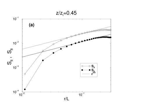
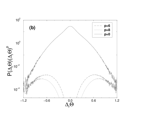
In Fig. 6(a) we report, for $z/z_{i}=0.45$ , the behaviors of the sixth and eight-order structure functions of temperature differences vs the separation between points (squares). Stright lines have the slope $\zeta_{\infty}=0.6$ . This is a further, direct, evidence of intermittency saturation. To investigate the statistical convergence of our sixth and eight-order moments, we reported in Fig. 6(b) the bulk contribution to such moments: $(\Delta_{r}\theta)^{p}P(\Delta_{r}\theta)$ , with $p=6$ and $p=8$ , $r/L\sim 7\times 10^{-2}$ in the inertial range of scales. For comparison $P(\Delta_{r}\theta)$ is also shown. Note that the maximum contribution to the moments six and eight comes from fluctuations $\Delta_{r}\theta$ in the region where $P(\Delta_{r}\theta)$ (i.e., $p=0$ ) is well resolved, i.e., our statistics appears reliable up to the order eight.

Once $\zeta_{\infty}$ is known, we evaluated from (6) the unknown function $Q$ . Such function is shown in Fig. 7 for two different values of $z$ within the mixed layer. Differences among the two curves are evident, signaling that $Q$ contains a dependence on the elevation $z$ . Such dependence can be associated to the relatively small shear present in our convective simulation (see Sec. 4) .
Further simulations spanning intermediate ABL (i.e. where both shear and buoyancy are important) have however to be performed in order to confirm the above last conclusion.

It is worth stressing that the scales $r$ at which we observe scaling behaviors are always larger than $\sim 8$ grid-points (i.e. sufficiently far from the scales directly affected by SGS parameterizations). Our attention being focused in a region sufficiently far from boundaries, this is another point in favor for the possible SGS independence of our results.

5.1.1 A link between geometry and statistics

Let us now conclude this section with a geometric point of view for the intermittency saturation (see also Celani et al, 2001a). As we shall see, the saturation exponent $\zeta_{\infty}$ is related to the fractal dimension, $D_{F}$ , of the set hosting the strong temperature fluctuations.
To do that, let us schematize in a very rough way our strong (i.e. larger than some $\sigma^{(z)}$ ) temperature fluctuations in the form of quasi-discontinuities (i.e. step functions). Each quasi-discontinuity will define a point (we are performing the analysis on planes at constant $z$ ) of given coordinate in our two-dimensional plane. The ensemble of all points defines the set, $S$ , hosting strong temperature fluctuations. Roughly, $S$ is formed by the intersection of our two-dimensional plane with the plume interfaces across which strong temperature jumps occur.
A useful indicator to characterize geometrically our set, $S$ , is the fractal dimension, $D_{F}$ , (see, e.g., Frisch (1995) for a presentation oriented toward turbulence problems). We briefly recall the standard way to define $D_{F}$ .

•

Take boxes of side, $r$ , and cover the whole plane at fixed $z$ . Denote with $N_{tot}$ the total number of those boxes;
•

Define the function $N(r)$ as the number of boxes containing at least one point of $S$ ;
•

For $r$ sufficiently small, one expects power law behavior for $N(r)$ in the form: $N(r)\sim r^{-D_{F}}$ , which defines the fractal dimension of $S$ .

Given the fractal dimension, $D_{F}$ , it is now easy to compute the probability, $Prob[|\Delta_{r;z}\theta|>\lambda\sigma^{(z)}]$ , of having strong (i.e. larger than some $\sigma^{(z)}$ ) temperature jumps within a certain distance $r$ . Indeed, by definition, we have:

Prob[|\Delta_{r;z}\theta|>\lambda\sigma^{(z)}]\equiv\frac{\mbox{favorable cases}}{\mbox{possible cases}}=\frac{N(r)}{N_{tot}}\sim\frac{r^{-D_{F}}}{r^{-2}}=r^{2-D_{F}}\;\;\;.

(16)

From (8) and (9) the identification $\zeta_{\infty}=2-D_{F}$ immediately follows. Notice that if one does not restrict the attention on the sole planes at constant $z$ , but focuses on the whole three dimensional space, the above relation becomes $\zeta_{\infty}=3-D_{F}^{\prime}$ where $D_{F}^{\prime}$ is the fractal dimension of the new set $S$ .

5.2 Statistics of weak temperature fluctuations

Let us now pass to investigate the statistics of well-mixed regions of the temperature field, corresponding to the inner parts of plumes that are likely to be present in our CBL (see again Fig. 1).
In these regions, fluctuations turn out to be very gentle and, as an immediate consequence, statistics is expected to be controlled in terms of single-scale fluctuations (see the Introduction). The best candidate to characterize, from a statistical point of view, weak fluctuations is thus the rescaling form given by (3).
To investigate whether or not our data are compatible with such rescaling, it is enough to verify whether there exist a number, $\alpha^{(z)}$ , (a priori dependent on the elevation $z$ within the mixed layer) such that, looking at $r^{\alpha^{(z)}}P(\Delta_{r;z}\theta)$ vs $\Delta_{r;z}\theta/r^{\alpha^{(z)}}$ for different values of $r$ , all curves collapse one on the other for each value of $z$ .
Our data support this behavior for the pdf cores (as expected, the rescaling (3) holds solely for weak fluctuations), as it can be observed in Fig. 2(c) (for $z/z_{i}=0.3$ ), in Fig. 3(c) (for $z/z_{i}=0.45$ ) and Fig. 4(c) (for $z/z_{i}=0.6$ ). In all cases, the values of $\alpha^{(z)}$ is $\sim 0.2$ , that means that $\alpha^{(z)}$ does not depend on $z$ . As the exponent $\zeta_{\infty}$ , $\alpha\equiv\alpha^{(z)}$ thus characterizes the entire mixed layer.

6 Conclusions and discussions

We have characterized, from a statistical point of view, both large and weak temperature fluctuations of a convective boundary layer simulated by a large eddy simulation model.
The main results of our study can be summarized as follows.

•

Large temperature fluctuations, occurring across plume interfaces, turn out to be strongly intermittent. This is the cause of the observed break down of mean field theories á la Kolmogorov, predicting a linear behavior of the scaling exponents, $\zeta_{p}$ , of the structure functions of temperature differences, vs the order $p$ . We found, on the contrary, a pdf rescaling which corresponds to a nonlinear shape of $\zeta_{p}$ vs $p$ , with $\zeta_{p}\to\zeta_{\infty}\equiv const$ for $p$ large enough. This behavior is named intermittency saturation, i.e. the strongest violation of dimensional predictions.
Hence, the concept of ‘typical fluctuation’ does not make sense: it is necessary to specify which part of the pdf of temperature differences is sampled for the definition of ‘typical fluctuation’.
•

Weak temperature fluctuations, characterizing the inner plume region where temperature is extremely well-mixed, have a self-similar character. This amounts to say that, despite the fact that many scales are excited in the well-mixed regions, the concept of ‘typical fluctuation’ here makes sense. In this case a simple rescaling characterizes the pdf core, which corresponds to a linear behavior of the curve $\zeta_{p}$ vs $p$ for small $p$ ’s. The slope of the straight line $\zeta_{p}$ vs $p$ is $\alpha\sim 0.2$ .
•

Exponents $\alpha$ and $\zeta_{\infty}$ appear to be independent on the elevation within the mixed layer. They are thus an intrinsic property of the entire mixed layer.
•

Statistics and geometry turn out to be intimately related. A simple relationship holds indeed between $\zeta_{\infty}$ and the fractal dimension, $D_{F}$ , of the set hosting the large temperature fluctuations: $\zeta_{\infty}=d-D_{F}$ where $d$ is the usual dimension of the physical space.
As for $\zeta_{\infty}$ , $D_{F}$ appears an intrinsic, i.e. $z$ -independent, property of the entire mixed layer.

It is worth stressing that the present scenario holds also for idealized, two-dimensional, models of scalar turbulence both passive (see Frisch et al (1999), Celani et al (2000) and Celani et al (2001a)) and active (see Celani et al (2001b)), simulated by means of direct numerical simulations. This fact naturally points toward the possible generality of the present statistical characterization for the entire class of scalar transport problems.

Finally, let us discuss a possible application of our results within boundary layer physics, and, more specifically, in the LES approach. As well known, one of the most challenging problem in the LES strategy is to find a proper way to describe the dynamical effect of small-scale unresolved motion on the resolved large scale dynamics. Recently, new approaches have emerged as alternatives to the eddy viscosity and similarity models (see, e.g., Meneveau and Katz, 2000). They construct the small-scale unresolved part of a total field (e.g., the velocity field) by extrapolating properties of the (resolved) coarse-grained field. A specific form for the subgrid scale field is thus postulated exploiting scale-invariance (i.e. inertial range scaling behavior) of the coarse-grained field. Note that, standard approaches postulate the form of the stress tensor rather than the structure of the unresolved field.
The mathematical tool which permits to perform such an interpolation is known as “fractal interpolation” (see Meneveau and Katz (2000) and references therein) where the free parameter of the theory is the fractal dimension of the field.
Up to now, many efforts have been devoted to exploit such strategy for the velocity fields. The latter exhibit however a multifractal structure (roughly speaking, an infinite set of fractal dimensions characterizes the whole field) and thus the fractal dimension parameter is a sort of ‘mean field’ description.
The suggestion arising from our results is that the same technique exploited for the velocity field appears successfully applicable in the convective case to the temperature field as well. Indeed, our results support a fractal structure of the temperature field. The situation seems to be even better than that for the velocity field. As we have stressed in the preceding sections, solely two exponents characterize most of the statistical properties of temperature fluctuations. We thus propose to schematize temperature fluctuations as a bi-fractal object (i.e., the simplest multifractal object) described by our two exponents $\alpha$ and $\zeta_{\infty}$ , and to generalize “fractal interpolation” to this case.
To do that, it seems necessary to investigate how the exponents we found for the analyzed experiment change by varying, e.g., the weight of buoyancy with respect to shear. We are currently working on this point and, as far as we remain on convective experiments, it seems that only small variations appear.
It should also be interesting to investigate what happens to the above scenario in stable stratified boundary layers. In that cases LES approach appears more delicate than in a CBL. Observations in field and/or in a wind tunnel should be thus necessary to investigate the problem.

References

Andrén, A., and C.-H. Moeng, 1993: Single-point closure in a neutrally stratified boundary layer. J. Atmos. Sci., 50, 3366-3379.

Bolgiano, R., 1959: Turbulent spectra in a stably stratified atmosphere. J. Geophys. Res., 64, 2226-2229.

Celani, A., A. Lanotte, A. Mazzino, and M. Vergassola, 2000: Universality and saturation of intermittency in passive scalar turbulence. Phys. Rev. Lett., 84, 2385-2388.

Celani, A., A. Lanotte, A. Mazzino, and M. Vergassola, 2001a: Fronts in passive scalar turbulence. Phys. Fluids, 13, 1768-1783.

Celani, A., A. Mazzino, and M. Vergassola, 2001b: Thermal plume turbulence. Phys. Fluids, 13, 2133-2135.

Frisch, U., 1995: Turbulence. The legacy of A.N. Kolmogorov. Cambridge University Press, 296 pp.

Frisch, U., A. Mazzino, and M. Vergassola, 1998: Intermittency in passive scalar advection. Phys. Rev. Lett., 80, 5532-5537.

Frisch, U., A. Mazzino, and M. Vergassola, 1999: Lagrangian dynamics and high-order moments intermittency in passive scalar advection. Phys. Chem. Earth, 24, 945-951.

Garratt, J.R., 1999: The atmospheric boundary layer. Cambridge University Press, 316 pp.

Meneveau, C. and J. Katz, 2000: Scale-Invariance and turbulence models for Large-eddy simulation, Annu. Rev. Fluid Mech., 32, 1-32.

Moeng, C.-H., 1984: A large-eddy-simulation model for the study of planetary boundary-layer turbulence, J. Atmos. Sci., 41, 2052-2062.

Moeng, C.-H. and J.C. Wyngaard, 1989: Evaluation of turbulent transport and dissipation closures in second-order modeling. J. Atmos. Sci., 46, 2311-2330.

Moeng C.-H., and P.P. Sullivan, 1994: A comparison of shear and buoyancy driven Planetary Boundary Layer flows. J. Atmos. Sci., 51, 999-1021.

Obukhov, A., 1949: Structure of the temperature field in turbulence. Izv. Akad. Nauk. SSSR. Ser. Geogr., 13, 55-69.

Pielke, R.A., 1984: Mesoscale Meteorological Modeling. Academic Press, 612 pp.

Shraiman B.I, and E.D. Siggia, 2000: Scalar turbulence. Nature, 405, 639-646.

Sullivan, P.P., J.C. McWilliams, and C.-H. Moeng, 1994: A subgrid-scale model for large-eddy simulation of planetary boundary layer flows. Bound. Layer Meteorol., 71, 247-276.

Acknowledgments
We are particularly grateful to Chin-Hoh Moeng and Peter Sullivan, for providing us with their LES code as well as many useful comments, discussions and suggestions. Helpful discussions and suggestions by A. Celani, R. Festa, C.F. Ratto and M. Vergassola are also acknowledged. This work has been partially supported by the INFM project GEPAIGG01 and Cofin 2001, prot. 2001023848. Simulations have been performed at CINECA (INFM parallel computing initiative).

List of Figures

1.

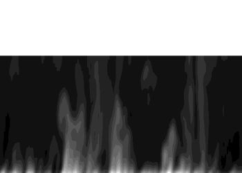
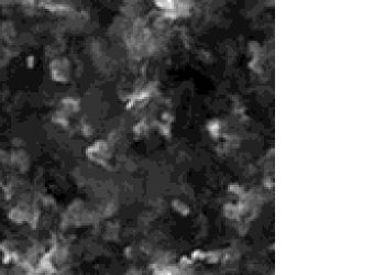
A typical snapshot of the potential temperature field $\theta$ , in the quasi-steady state of a convective boundary layer simulated by a Large Eddy Simulation with resolution $128^{3}$ . Above: vertical cross-section restricted to the mixed layer; below: horizontal cross-section inside the mixed layer. Colors are coded according to the intensity of the field: white corresponds to large temperature, black to small ones. Plumes and well-mixed regions are clearly detectable.
2.

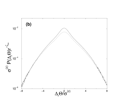
The pdf’s $P(\Delta_{r;z}\theta)$ , for two values of $r$ inside the inertial range of scales (dotted lines: $r/L=0.22$ ; continuous line: $r/L=0.11$ , $L$ being the side of the (squared) simulation domain) and $z/z_{i}=0.3$ , $z_{i}$ being the elevation of the mixed layer top. (a): pdf’s are shown without any $r$ -dependent rescaling; (b) the pdf is multiplied by the factor $\sigma^{(z)}r^{-\zeta_{\infty}}$ with $\zeta_{\infty}\sim 0.6$ : the collapse of the curves indicate the asymptotic behavior $P(\Delta_{r;z}\theta)\sim r^{\zeta_{\infty}}$ for large $\Delta_{r;z}\theta$ , that means saturation of temperature scaling exponents (see, and (6), (8) and (9)); (c) pdf’s are multiplied by the factor $r^{\alpha^{(z)}}$ while $\Delta_{r;z}\theta$ by $r^{-\alpha^{(z)}}$ : the collapse of pdf cores indicates the validity of (3) that is equivalent to the linear behavior of low-order temperature scaling exponents (see (4)).
3.

As in Fig. 2 but for $z/z_{i}=0.45$ .
4.

As in Fig. 2 but for $z/z_{i}=0.6$ .
5.

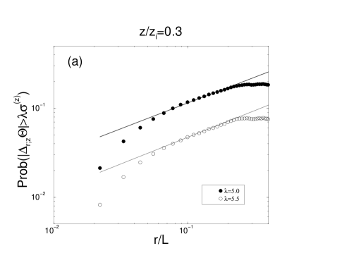
The cumulated probabilities $Prob[|\Delta_{r;z}\theta|>\lambda\sigma^{(z)}]$ for two values of $\lambda$ are shown for (a): $z/z_{i}=0.3$ and (b): $z/z_{i}=0.6$ . The slope of these curves (continuous line) are compatible with the exponent $\zeta_{\infty}\sim 0.6$ . The error bar on this slope is of the order of $0.1$ , evaluated by means of the local scaling exponents (on half-decade ratios) as customary in turbulence data analysis.
6.

(a) Sixth and eight-order structure functions of temperature differences vs the separation between points (squares). Stright lines have the slope $\zeta_{\infty}=0.6$ . (b) The bulk contribution to the moments $p=6$ and $p=8$ , $(\Delta_{r}\theta)^{p}P(\Delta_{r}\theta)$ , with $r/L\sim 1.1\times 10^{-1}$ in the inertial range of scales. For comparison $P(\Delta_{r}\theta)$ (i.e. for $p=0$ ) is also shown. Note that the maximum contribution to the moments six and eight comes from fluctuations $\Delta_{r}\theta$ in the region where $P(\Delta_{r}\theta)$ is well resolved. This proves the reliability of our statistics to compute moments up to the order eight.
7.

The function $Q$ defined in (6) is shown for two different values of $z$ within the mixed layer: $z/z_{i}=0.3$ (dotted line) and $z/z_{i}=0.6$ (continuous line). Differences in the shape of these two curves, reveal that $Q$ contains a dependence on the elevation, $z$ , within the mixed layer.