Strong-field terahertz-optical mixing in excitons

Abstract

Driving a double-quantum-well excitonic intersubband resonance with a terahertz (THz) electric field of frequency $\omega_{THz}$ generated terahertz optical sidebands $\omega=\omega_{THz}+\omega_{NIR}$ on a weak NIR probe. At high THz intensities, the intersubband dipole energy which coupled two excitons was comparable to the THz photon energy. In this strong-field regime the sideband intensity displayed a non-monotonic dependence on the THz field strength. The oscillating refractive index which gives rise to the sidebands may be understood by the formation of Floquet states, which oscillate with the same periodicity as the driving THz field.

Electromagnetically-induced coherent quantum effects in semiconductor systems include Rabi oscillations in donors[1] and quantum dots[2], and electromagnetically-induced transparency in quantum wells[3]. In these effects, to induce coherence the driving field must overcome dephasing processes. Thus, the Rabi frequency $\mu E$ must be greater than the dephasing rates $\gamma$: $\mu E>\hbar\gamma$, where $\mu$ is the dipole moment and $E$ is the electric field strength.

If the field strength is increased still further, a strong-field regime is encountered as the Rabi energy becomes comparable to the photon energy: $\mu E\geq\hbar\omega$. Previous studies into this regime have looked at atoms in microwave cavities[4, 5] and strong laser fields[6]. Since atomic excited states are near the continuum, strong-field effects manifest themselves as nonmonotonic multi-photon ionization rates as a function of field strength.

However, the atoms are ionized, meaning the bound states do not exist after the microwave or laser field is turned on. Multi-photon ionization is an inescapable result of driving excited atomic levels which get closer and closer together.

There is a rich body of theoretical predictions on the effect of strong fields on the bound states of a quantum system[7, 8]. In quantum wells, upper states get further and further apart. Thus the strong-field condition can be satisfied by resonantly driving the lowest subbands of a quantum well at THz frequencies. Yet the quantum well is far deeper than the Rabi energy, so the bound states still survive.

We describe experiments in which a near-infrared (NIR) probe laser beam is mixed with a terahertz (THz) pump beam in a gated, asymmetric double quantum well (DQW). The THz field couples to an excitonic intersubband excitation while the NIR field couples to an excitonic interband excitation. Applying a DC voltage to the gates brings the intersubband transition into resonance with the THz field, and the interband transition into resonance with the NIR field. When these resonance conditions are met the NIR probe is modulated resulting in the emission of optical sidebands which appear at frequencies $\omega_{sideband}=\omega_{NIR}+n\omega_{THz}$ where $\omega_{NIR}$ ($\omega_{THz}$) is the frequency of the NIR (THz) beam and $n=\pm 1,2,\ldots$. Strong-field effects manifest themselves as non-monotonic sideband intensities as a function of THz field strength.

The sample consisted of an active region, gates, and a distributed Bragg reflector (DBR). The active region consisted 5 periods of DQW, each consisting of a 120 Å GaAs QW and a 100 Å GaAs QW separated by a 25 Å Al_0.2Ga_0.8As tunnel barrier. Each period was separated by a 300 Å Al_0.3Ga_0.7As barrier. The active region was sandwiched between two gates, each consisting of a Si delta-doped 70 Å QW with carrier density $\approx 1\times 10^{12}$ cm^-2. The gates were separated from the active region by 3000 Å Al_0.3Ga_0.7As barriers. Since the gate QWs are much narrower than the active DQWs, the gate QWs are transparent to both the THz and NIR beams. The gated DQWs were grown on top of a DBR which consisted of 15 periods of 689 Å AlAs and 606 Å Al_0.3Ga_0.7As. It had a low-temperature passband nearly centered on the low-temperature bandgap of the DQW, making it about 95% reflective for the NIR probe beam and sidebands.

We etched a mesa and annealed NiGeAu ohmic contacts to the gate QWs. The sample was then cleaved into a 1 mm wide strip, 8 mm long. We then cleaved a 400 $\mu$m-thick wafer of crystal sapphire substrate material into a $1\times 5$ mm strip, oriented with the optically slow axis along the long dimension. The sapphire was mechanically pressed against the surface of the sample with a beryllium copper clip as shown in Fig. 1. At cryogenic temperatures sapphire is index-matched to GaAs and transparent at THz wavelengths. At the same time, sapphire is transparent to the NIR probe. Pressing the sapphire against the sample forms a rectangular dielectric waveguide with half of the waveguide defined by the sample substrate and the other half defined by the sapphire. The epilayer containing the active region lies in the middle of the heavily over-moded waveguide. This results in much higher fields at the active region than would be possible without the sapphire, where the active region would be at the edge of a dielectric waveguide.

The sample was cooled to 21 K in a closed-cycle He cryostat. The 1 kW THz beam from a free-electron laser is polarized in the growth direction, propagated in the QW plane and focused by a 90^o off-axis parabolic mirror (F/1) into the edge of the waveguide. The maximum THz electric field strength at the focus is estimated to be between $\approx 5-20$ kV/cm, where our uncertainty comes from uncertainty of the exact size of the mode in the waveguide. The THz power can be continuously varied by a pair of wire-grid polarizers.

NIR light from a continuous-wave Ti:sapphire laser is chopped by an acousto-optic modulator into 25 $\mu$s pulses which overlap the 5 $\mu$s FEL pulses at maximum repetition rate of 1.5 Hz. The vertically-polarized NIR beam propagates normal to the THz beam, and was focused (F/10) at a power density of $\approx$ 5 W/cm² to the same small interaction volume in the sample. The reflected beam, sidebands, and photoluminescence (PL) are analyzed by a second polarizer, dispersed by a 0.85 m double-monochromator, and detected by a photomultiplier tube.

Previous work [9, 10] showed that sideband generation is enhanced when the NIR field resonantly couples the vacuum state $|0\rangle$ with an exciton $|1\rangle$, and the THz field resonantly couples with the intersubband transition between excitons $|1\rangle$ and $|2\rangle$. The exciton states can be labelled as E_μHH_νX, indicating an exciton consisting of an electron in conduction subband $\mu$ and a heavy hole in valence subband $\nu$. Changing the DC electric field tunes the excitonic intersubband transition into resonance with the THz field, as shown in Fig. 2. The sideband resonance we focused on is E2HH2X-E2HH3X, a peak assignment made by comparing low-field sideband spectroscopy with a nonlinear susceptibility calculation for excitons[10].

Fig. 3 shows the dependence on THz field strength of sideband generation at various THz frequencies. Each curve was taken at a gate bias near the E2HH2X-E2HH3X resonance[10]. The most striking feature is the non-monotonic behavior in the strong-field regime when the Rabi energy is comparable to the photon energy. Clearly at lower frequencies the power dependence rolls over at a lower field strength.

By sitting at the peak NIR frequency for E2HH2X-E2HH3X and varying the DC gate voltage we took THz power dependence scans at various THz detunings $E_{2}-E_{1}-\hbar\omega_{THz}$ where $E_{2}$ ($E_{1}$) is the energy of the upper (lower) exciton state. The results are shown in Fig. 4. As the detuning is varied, so does the shape of the THz field dependence.

The power dependence cannot be explained by a nonlinear susceptibility, which is inherently a low-field theory because it relies on a Taylor expansion about the field strength [11]. Saturation effects[12] in a nonlinear susceptibility can only come about when contributions from virtual transitions initiated from excited states $|1\rangle$ or $|2\rangle$ are comparable to those initiated from the vacuum $|0\rangle$. However the populations of excited states $|1\rangle$ or $|2\rangle$ are never significant compared with $|0\rangle$ in our undoped sample and weak NIR beam. Therefore a nonlinear susceptibility can only predict a linear (quadratic) dependence of sideband intensity on THz power (field strength).

The following simple, phenomenological, three-state model captures qualitative features of the dependence of sidebands on THz power. The Hamiltonian $H_{0}$ has eigenstates $\phi_{0}(x,z)$, $\phi_{1}(x,z)$, and $\phi_{2}(x,z)$ with eigenenergies $E_{0}=0$, $E_{1}$, and $E_{2}$, respectively. Near the experimental resonance, the effect of the DC voltage is to tune $\phi_{2}$ while the other $\phi_{1}$ remains relatively unchanged[10]. The two exciton states $\phi_{1}(x,z)$ and $\phi_{2}(x,z)$ are coupled by the $z$-dipole operator for the DC and THz fields. The two upper states $\phi_{1}(x,z)$ and $\phi_{2}(x,z)$ are coupled to the ground state by the $x$-dipole operator for the NIR field.

Therefore, the x and z matrices are

$$z=\left({\begin{array}[]{ccc}0&0&0\\ 0&0&z_{12}\\ 0&z_{21}&z_{22}\end{array}}\right)x=\left({\begin{array}[]{ccc}0&x_{01}&x_{02}\\ x_{10}&0&0\\ x_{20}&0&0\end{array}}\right)$$ (7)

All the nonzero terms $x_{\alpha\beta}=\langle\phi_{\alpha}|x|\phi_{\beta}\rangle$ and $z_{\alpha\beta}=\langle\phi_{\alpha}|z|\phi_{\beta}\rangle$ are set equal to unity. The Hamiltonian is

$$H=H_{0}+zE_{\omega}\cos{\omega t}+x\lambda E_{\Omega}\cos{\Omega t}$$

where $E_{\omega}$ represents the strong THz electric field strength and $E_{\Omega}$ represents the weak NIR electric field. We solved the Hamiltonian nonperturbatively within a Floquet formalism for $\lambda=0$, while the weak probe was added later using time-dependent perturbation theory.

The solutions to the Schrodinger equation for the time-periodic Hamiltonian have the form[13]

$$\varphi_{i}(z,t)=e^{-i\epsilon_{i}t/\hbar}u_{i}(z,t),u(z,t)=u(z,t+\frac{2\pi}{\omega})$$ (8)

where $u_{i}(z,t)$ has the same periodicity as the driving frequency and and $\epsilon_{i}$ is called the quasienergy. The states $\varphi_{i}(z,t)$ are called Floquet states and are mathematically analogous to Bloch states for a spatially-periodic Hamiltonian. Meanwhile the quasienergies are analogous to the crystal momenta of Bloch theory.

The spatial-dependence of the wavefunction $\varphi_{i}(z,t)$ can be expanded in terms of the original eigenstates $\phi_{\alpha}(z)$, and the time-dependence can be Fourier-expanded

$$\varphi_{i}(z,t)=e^{-i\epsilon_{i}t/\hbar}\sum_{\alpha,n}c^{i}_{\alpha,n}e^{-in\omega t}\phi_{\alpha}(z)$$ (9)

The coefficients $c^{i}_{\alpha,n}$ are what will determine the part of the index of refraction which will oscillate at particular multiples of $\omega$. Solving for these coefficients is the key to understanding the power dependence of the sideband. These Floquet coefficients are closely related to the photon-assisted tunnelling sidebands which appear in the irradiated current-voltage curves in superconducting weak-link junctions[14] and coupled quantum wells[15].

The time-dependent Schrodinger equation can be cast in terms of the Floquet operator $F=H-i\hbar\frac{\partial}{\partial t}$, which can be written as a matrix of the form[8]

$$F=\left({\begin{array}[]{ccccc}\ddots&[\mu]&0&0&0\\ {[\mu]}&[H_{0}]-\hbar\omega&[\mu]&0&0\\ 0&[\mu]&[H_{0}]&[\mu]&0\\ 0&0&[\mu]&[H_{0}]+\hbar\omega&[\mu]\\ 0&0&0&[\mu]&\ddots\end{array}}\right)$$ (10)

where $[H_{0}]$ and $[\mu]$ are matrix representations of the operators $H_{0}$ and $\mu$ in the $|\phi_{\alpha}\rangle$ basis. In practice the Floquet matrix must be truncated up to $\pm N$ photons. $N$ can be made arbitrarily large for an arbitrarily precise result at high field strengths. The solution to the Schrodinger equation for a time-periodic Hamiltonian reduces to finding the eigenvalues and eigenvectors of the Floquet matrix (10). Other than the $\pm N$ truncation the solution involves no perturbation or rotating-wave approximations. Here we used $N=16$ photons.

The Floquet solutions are labeled $\varphi_{i}(x,z,t)$ with $i=0,1,2$, and expanded as in (9). Their expansions are explicitly expressed for clarity:

$$\varphi_{0}(x,z,t) = \phi_{0}(x,z)$$

$$\varphi_{1}(x,z,t) = e^{i\epsilon_{1}t/\hbar}\sum_{n}e^{-in\omega t}[c^{1}_{1,n}\phi_{1}(x,z)+c^{1}_{2,n}\phi_{2}(x,z)]$$

$$\varphi_{2}(x,z,t) = e^{i\epsilon_{2}t/\hbar}\sum_{n}e^{-in\omega t}[c^{2}_{1,n}\phi_{1}(x,z)+c^{2}_{2,n}\phi_{2}(x,z)]$$

The ground state $\phi_{0}(x,z)$ is not coupled by the the strong field to the 2-d subspace spanned by $|\phi_{1}\rangle$ and $|\phi_{2}\rangle$. Therefore the coefficients for the Floquet state $\varphi_{0}(x,z,t)$ vanish except $c^{0}_{0,0}=1$. In other words, the ground vacuum state remains untouched by the intense THz field.

The dipole response of the Floquet states to the weak NIR probe is calculated perturbatively. The state of the system with both driving fields $\psi(x,z,t)$ can be expanded in terms of the Floquet states $\varphi_{i}(x,z,t)$ to first order. Discarding second order terms and anti-resonant contributions, the dipole expectation is given by

$$\langle\psi|x|\psi\rangle=E_{\Omega}e^{-i\Omega t}\sum_{i=1}^{2}\frac{\langle\varphi_{0}|x|\varphi_{i}\rangle\langle\varphi_{i}|x|\varphi_{0}\rangle}{\epsilon_{i}-\hbar\Omega}$$ (11)

The form of (11) is the same as the linear susceptibility of an undriven system, except the states $\varphi_{i}$ are oscillating Floquet states instead of stationary states. Explicitly expanding the Floquet states in the numerator gives us an expression for the polarization

$$x(t)=E_{\Omega}e^{-i\Omega t}\sum_{i=1}^{2}\mathop{\sum_{n,\alpha}}_{m,\beta}\frac{c^{i}_{n,\alpha}c^{i}_{m,\beta}e^{-i(n-m)\omega t}x_{0\beta}x_{\alpha 0}}{\epsilon_{i}-\hbar\Omega}$$ (12)

The $+1\omega$ sideband is given by the Fourier component of $x(t)$ oscillating at the frequency $\Omega+1\omega$. Also, for the resonant condition illustrated in Fig. 2, $\hbar\omega\approx\epsilon_{1}$, so we keep only the $i=1$ term in the sum (12). This condition is satisfied when $n-m=1$. Thus we obtain an expression for the sideband polarization

$$x_{sideband}(t)=\frac{E_{\Omega}e^{-i(\Omega+\omega)t}}{\epsilon_{1}-\hbar\Omega}\sum_{n,\alpha,\beta}c^{1}_{n+1,\alpha}c^{1}_{n,\beta}x_{0\beta}x_{\alpha 0}$$ (13)

The intensity of the sideband is proportional to $x_{sideband}^{2}$. This is plotted vs. field strength for various detunings in Fig. 5. The detuning parameter $d$ is the level spacing normalized by the photon energy of the strong field, $d=\frac{E2-E1}{\hbar\omega}$.

Our model captures the rollover of the resonant power dependence up to field strengths of around $\frac{\mu E}{\hbar\omega}\approx 1.5$. Given a calculated excitonic intersubband dipole of $\frac{\mu}{e}=$ 12 nm[10], the strong-field condition is met at a THz field of 5 kV/cm. However, experimentally the sideband never completely disappears, a striking prediction of the theory. It is unlikely that a 3-state simplification is entirely valid because there is a spectrum of other exciton states as well as an electron-hole continuum that may provide significant off-resonant contributions.

To summarize, we drove an quantum-well excitonic intersubband transition with an intense THz laser field in a regime where the Rabi energy was comparable to the photon energy. The nonlinear mixing between the THz pump and a weak NIR probe displayed a nonmonotonic dependence on THz power, which could not be explained by a conventional nonlinear susceptibility. Rather, the excitons were dressed by the THz field, a process which we described in a simple three-level model in which the interaction between excitons and the THz field is solved non-perturbatively within the Floquet formalism.

This research is funded by NSF-DMR 0070083.

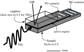
FIG. 1.: Processed waveguide device and optical coupling scheme.

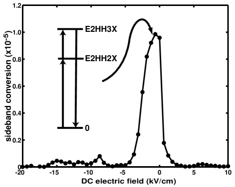
FIG. 2.: The dc electric field dependence of sideband at $\hbar\omega_{NIR}=1547$ meV and $\omega_{THz}=1.5$ THz (6.2 meV). The inset illustrates the resonant condition in which the NIR field is resonant with the E2HH2 exciton and the THz field resonantly couples the E2HH2 and E2HH3 excitons.

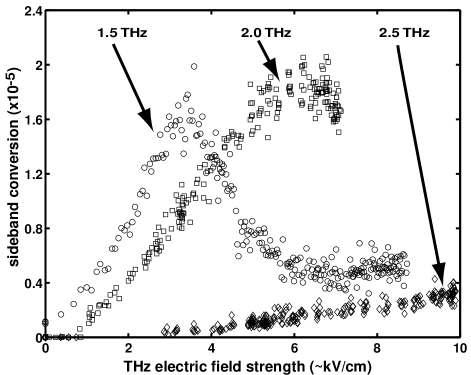
FIG. 3.: Resonant THz field strength dependence of sideband generation at 1.5 THz, 2.0 THz, and 2.5 THz (6.2 meV, 8.2 meV, 10.4 meV). The absolute THz electric field scale is accurate only to within a factor of 2.

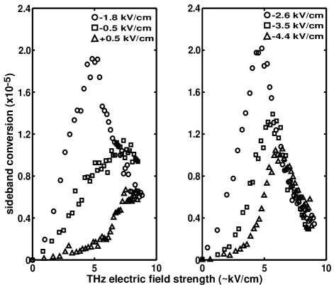
FIG. 4.: THz field strength dependence of $n=1$ sideband for $\omega_{NIR}$=1548 meV, $\omega_{THz}=1.5$ THz (6.2 meV) at various DC electric field detunings from the resonance condition illustrated in Fig. 2. The absolute THz electric field scale is accurate only to within a factor of 2.

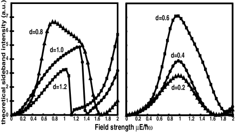
FIG. 5.: Sidebands calculated by evaluating the square of (13) at various detuning parameters LEFT: $d=\frac{E2-E1}{\hbar\omega}=0.8,1.0,1.2$, RIGHT: $d=\frac{E2-E1}{\hbar\omega}=0.2,0.4,0.6$.

REFERENCES

- [1] B.E. Cole, J.B. Williams, B.T. King, M.S. Sherwin. Nature, 410(6824):60, 2001.
- [2] T. H. Stievater, X. Li, D.G. Steel, D. Gammon, D.S. Katzer, D. Park, C. Piermarocchi, L.J. Sham. Phys. Rev. Lett, 87(13):133603, 2001.
- [3] G. B. Serapiglia, E. Paspalakis, C. Sirtori, K.L. Vodopyanov, C.C. Phillips. Phys. Rev. Lett., 84(5):1019, 2000.
- [4] K.A.H. van Leeuwen, G. v. Oppen, S. Renwick, J.B. Bowlin, P.M. Koch, R.V. Jensen, O. Rath, D. Richards, J.G. Leoplod. Phys. Rev. Lett, 55(21):2231, 1985.
- [5] A. Haffmans, R. Blumel, P.M. Koch, L. Sirko. Phys. Rev. Lett, 73(2):248, 1994.
- [6] Ed. M. Gavrila. Atoms in Intense Laser Fields. Academic Press, Boston, 1992.
- [7] K. Johnsen, A.-P. Jauho. Phys. Rev. Lett, 83(6):1207, 1999.
- [8] T. Fromherz. Phys. Rev. B, 56(8):4772, 1997.
- [9] M.Y. Su, S. Carter, M.S. Sherwin, A. Huntington, L.A. Coldren. LANL eprint archive, physics/0201038, 2002.
- [10] M.Y. Su, S. Carter, M.S. Sherwin, A. Huntington, L.A. Coldren. To be published. Draft available at http://lizardmouth.net/msu/physics/papers/papers.htm.
- [11] R. Boyd. Nonlinear optics. Academic Press, San Diego, 1992.
- [12] J.N. Heyman, K. Craig, B. Galdrikian, M.S. Sherwin, K. Campan, P.F. Hopkins, S. Fafard, A.C. Gossard. Phys. Rev. Lett, 72(14):2183, 1997.
- [13] J.H. Shirley. Phys. Rev., 138:979, 1965.
- [14] P.K. Tien and J.P. Gordon. Phys. Rev., 129:647, 1963.
- [15] H. Drexler, J.S. Scott, S.J. Allen, K.L. Campman, A.C. Gossard. Appl. Phys. Lett., 67(19):2816, 1995.