Abstract

Metabolic control analysis (Kacser & Burns (1973). Symp. Soc. Exp. Biol. 27, 65-104; Heinrich & Rapoport (1974). Eur. J. Biochem. 42, 89-95) was developed for the understanding of multi-enzyme networks. At the core of this approach is the flux summation theorem. This theorem implies that there is an invariant relationship between the control coefficients of enzymes in a pathway. One of the main conclusions that has been derived from the summation theorem is that phenotypic robustness to mutation ( e.g. dominance ) is an inherent property of metabolic systems and hence does not require an evolutionary explanation (Kacser & Burns (1981). Genetics. 97, 639-666; Porteous (1996). J. theor. Biol. 182, 223-232 ). Here we show that for mutations involving discrete changes ( of any magnitude ) in enzyme concentration the flux summation theorem does not hold. The scenarios we examine are two-enzyme pathways with a diffusion barrier, two enzyme pathways that allow for enzyme saturation and two enzyme pathways that have both saturable enzymes and a diffusion barrier. Our results are extendable to sequential pathways with any number of enzymes. The fact that the flux summation theorem cannot hold in sequential pathways casts serious doubts on the claim that robustness with respect to mutations is an inherent property of metabolic systems.

1. Introduction

How do changes in enzyme properties alter the physiological phenotype? Such knowledge is a key component in understanding the relation between genotype and phenotype. The two main approaches to this problem have developed into fields known as metabolic control analysis ( MCA ) [Kacser & Burns, 1973, Heinrich & Rapoport, 1974, Kacser et al., 1995] and biochemical systems theory ( BST )  [Savageau, 1976, Savageau & Sorribas, 1989]. Results from MCA have had extensive influence in biochemistry, genetics and evolution ( for an overview see the entire issue of J. theor. Biol., 182:3 , 1996 ). The cornerstone of the MCA approach is a theoretical result referred to as the flux summation theorem. The biological interpretation of the summation theorem is that there are systemic constraints inherent in metabolic pathways; these constraints limit the magnitude of the effects that changes in enzyme activity can have on flux through a pathway. The existence of such constraints has two implications. In the first place, the summation theorem implies that in general the control of flux in a pathway is shared between enzymes. Hence rate limiting enzymes are rare [Kacser, 1995]. Secondly, the theorem implies that on the average, mutations that change enzyme concentrations will have a small effect on flux. This implication has important consequences in evolutionary theory and genetics. It means that phenomena that fall under the rubric of phenotypic robustness to mutations ( such as selective neutrality, canalization and dominance ) are inherent properties of metabolic systems and are not a result of evolution. This MCA argument was originally made in reference to the case of dominance, stating that dominance is an inherent property of metabolic pathways and not a result of evolution [Kacser & Burns, 1981, Keightley, 1996, Porteous, 1996].

At the core of the MCA approach is a measure of the control exerted by each enzyme on flux through a pathway. The control coefficient $C_{i}^{J}$ measures how important each enzyme is in its ability to affect steady-state flux via changes in enzyme concentration. In its original formulation [Kacser & Burns, 1973] the control coefficient was defined as

$$C_{i}^{J}={\frac{\delta J}{J}}/{\frac{\delta E_{i}}{E_{i}}},$$ (1)

where $J$ is the steady state flux of metabolites through the pathway (net rate of product formation at the end of a pathway), $E_{i}$ is the concentration of enzyme $i$, $\delta E_{i}$ is a discrete change in enzyme concentration and $\delta J$ is the resultant change in flux. Hence $C_{i}^{J}$ is basically a ratio of percentage change in a pathway’s steady state flux to the corresponding percentage change in enzyme concentration.

Theoretical results that contradict or object to different conclusions derived within MCA have been posed several times [Cornish-Bowden, 1987, Giersch, 1988, Savageau & Sorribas, 1989, Savageau, 1992, Grossniklaus et al., 1996, Kholodenko et al., 1998]. In each case the possible misrepresentation of non-linearities in MCA has appeared in a different guise. In the first place, Cornish-Bowden (1987) showed that in a sequential pathway if the maximal rate $V_{max}$ of consecutive enzymes are sequentially decreasing then dominance is not a necessary property of the pathway. Hence the possibility exists that dominance can evolve. This objection was rejected in MCA on grounds that the specific arrangement of kinetic values suggested is a special case that is very unlikely to occur by chance [Kacser, 1987]. A second set of objections was then put forth by Savageau and Sorribas (1989, 1992). They argued that in pathways exhibiting non-linear behavior that arises from properties such as enzyme-enzyme interactions, feedback loops or non-sequential pathway structure it can be shown that dominance is not inherent to the pathway. Based on disagreements on the mathematical models used, this second objection was rejected by MCA proponents [Kacser, 1991, Kacser, 1995]. Nevertheless more recent work indirectly corroborates this objection [Grossniklaus et al., 1996, Kholodenko et al., 1998].

The present paper deals with problems involving the biological in-applicability of MCA precepts. We show that for discrete changes ( of any magnitude ) in enzyme concentration, the flux summation theorem does not hold. This means that contrary to the MCA allegations, there are no a-priori constraints that would require the magnitude of mutational effects to be small. Furthermore these results re-open the possibility that phenotypic robustness to mutations ( e.g. dominance ) is not an inherent property of metabolic pathways and can be a result of evolution.

Our conclusions do not necessarily imply that the summation theorem is inherently false as an isolated mathematical proposition. Rather that it has been applied to the wrong context. This erroneous application arises due to two main disparities. In the first place, the argument for the summation theorem in the original Kacser and Burns paper (1973) is derived using a discrete formulation. However, in most subsequent work ( e.g. Kacser & Burns 1981 ) a continous formulation of the theorem is used. Hence the discrete proof for the summation theorem does not correspond to the continous form in which it is frequently used. In the second place, mutations necessarily involve discrete changes in enzyme activity. Hence, whether a continous version of the summation theorem holds or not ( which it would in cases where the flux function is homogenous, see Giersch 1988 ) does not say anything about whether a pathway will be robust or exhibit dominance with respect to discrete changes. In order for a pathway to be robust with respect to discrete changes, the discrete version of the summation theorem has to hold. In this paper we show that for dicrete changes of any size the discrete version does not hold, and hence that robustness is not an inherent property of a metabolic pathway.

The matter addressed here has been a subject of debate for thirty years. In order to be clear about the objects that we treat and the mathematical properites that pertain to them a rigorous approach to the problem was necessary. The main assumptions and implications we derived are summarized as follows:  

INITIAL ASSUMPTION

Assumption 0.

The metabolic pathways studied are two-enzyme pathways. They have one input and one output and can reach a steady state flux.

CASE A : DIFFUSION LIMITED PATHWAYS

Assumption 1.

Maximal rate of input into the metabolic pathway is limited by a diffusion process.

Implication 1.

The flux summation theorem does not hold.

CASE B : SEQUENTIAL PATHWAYS THAT ALLOW FOR ENZYME SATURATION

Assumption 1.

The two enzymes are near saturation.

Implication 1.

The flux summation theorem does not hold.

CASE C : NUMERICAL ANALYSIS OF PATHWAYS WITH REVERSIBLE MICHAELIS-MENTEN KINETICS

Assumption 1.

Each enzyme in the pathway behaves according to reversible Michaelis-Menten enzyme kinetics. Isolated Michaelis-Menten enzymes do allow for enzyme saturation. Note that such kinetics are manifest in empirical studies of isolated enzymes in vitro.

Assumption 2.

When Michaelis-Menten enzymes are placed in the context of a multi-enzyme pathway, their kinetic mechanisms do not change. This is a pure assumption.

Assumption 3.

Maximal rate of input into the metabolic pathway is limited by a diffusion process. As in assumption 1, this is is an assumption that is empirically justified [Tralau et al., 2000].

Numerical Result 1.

In regimes where both enzymes are saturated the summation theorem does not hold.

Numerical Result 2.

In regimes where flux is near the diffusion limited rate, the summation theorem does not hold.

Assumption 4.

Mutations can cause heritable variation in the catalytic turnover rate $k_{cat}$ of an enzyme.

Numerical Result 3.

The control of a pathway can be switched from one enzyme to another via mutations affecting $k_{cat}$. Each enzyme can be the sole controlling enzyme of a pathway.

The main reason for the restricted applicability of the summation theorem is the fact that for its construction the non-linear interaction effects on flux were ignored. It is precisely the interaction effects between enzymes that lead to the manifestation of interaction effects ( epistasis ). Furthermore it is the interposition of the non-linear properties of enzymes that allow for the evolution of control.

2.  Mathematical Introduction

2.1. The conception of control in MCA

Upon devising MCA, as Kacser and Burns put it, it was necessary to place the understanding of individual enzyme behavior into the context of a “metabolic society” composed of several enzymes [Kacser & Burns, 1979]. In accordance to this goal, one of the objectives of metabolic control analysis was to ascertain what role each enzyme could play in affecting steady state flux in a particular metabolic pathway. Specifically, how important each enzyme is in its ability to affect steady state flux via the regulation of the enzyme concentration. Hence the use of the control coefficient as $C_{i}^{J}={\displaystyle\frac{\delta J}{J}/\displaystyle\frac{\delta E_{i}}{E_{i}}}$, which is a non-dimensionalized sensitivity measure that shows the ratio of proportional change in flux to proportional change in enzyme concentration.

2.2. The flux summation theorem

One of the central tenets of metabolic control theory has been that the sum of the control coefficients in a pathway with $n$ enzymes equals one. That is,

$$\sum_{i=1}^{n}C_{i}^{J}=1.$$ (2)

Equation (2) is commonly referred to as the flux summation theorem and was derived by Kacser and Burns using the following form of reasoning:

Given an unbranched chain of $n$ enzyme catalyzed reactions, if we were to increase the concentration $E_{i}$ of enzyme $i$ by the proportional ratio ${\delta E_{i}}/{E_{i}}$, the change in flux due to enzyme $i$ would be given by rearranging (1) to give:

$$\mbox{For all enzymes $i$ :}~{}\left({\frac{\delta J}{J}}\right)_{i}=\left(\frac{\delta E_{i}}{E_{i}}\right)C_{i}^{J}.$$ (3)

If $\delta E_{i}/E_{i}=\alpha$ , where $\alpha$ is a constant, one could consider the case where all enzyme concentrations are changed by the constant proportion $\alpha$. In such a case Kacser and Burns assume the following equation:

$$\frac{\delta J}{J}=\sum_{i=1}^{n}\left(\frac{\delta J}{J}\right)_{i}.$$ (4)

Hence, using (4), (3) and $\alpha={\delta E_{i}}/E_{i}$ ;

$$\frac{\delta J}{J}=\sum_{i=1}^{n}\alpha\,C_{i}^{J}=\alpha\sum_{i=1}^{n}C_{i}^{J}.$$ (5)

Separately, the assumption is made that if all enzyme concentrations are uniformly changed by $\alpha$ , then

$$\frac{\delta J}{J}=\alpha.$$ (6)

Substituting equation (6) into (5) we obtain equation (2):

$$\sum_{i=1}^{n}C_{i}^{J}=1.$$

For a clearer view, the Kacser and Burns derivation of (2) can be summarized in the following conditionals:

$$\begin{array}[]{l}\left(\begin{array}[]{c}(\ref{7b});~{}(\mbox{ Definition })~{}~{}~{}~{}\left[~{}\left({\frac{\delta J}{J}}\right)_{i}=\left(\frac{\delta E_{i}}{E_{i}}\right)C_{i}^{J}~{}\right]~{}~{}\wedge{}\\ \\ (\ref{18});~{}(\mbox{ Assumption })~{}~{}~{}~{}\left[~{}\frac{\delta J}{J}=\sum_{i=1}^{n}\left(\frac{\delta J}{J}\right)_{i}~{}\right]~{}~{}\wedge{}\\ \\ \mbox{( Restriction )}~{}~{}~{}~{}(\forall i):[~{}{\delta E_{i}}/E_{i}=\alpha~{}]\end{array}\right)\\ \\ ~{}~{}~{}~{}~{}~{}~{}~{}~{}~{}~{}~{}~{}~{}~{}~{}~{}~{}~{}~{}~{}~{}~{}~{}~{}~{}~{}~{}~{}~{}~{}~{}~{}~{}~{}~{}~{}~{}~{}~{}\Rightarrow\left(\begin{array}[]{r}(\ref{19});~{}~{}~{}~{}\left[~{}\frac{\delta J}{J}=\alpha\sum_{i=1}^{n}C_{i}^{J}~{}\right]\end{array}\right).\end{array}$$ (7)

$$\begin{array}[]{l}\left(\begin{array}[]{c}(\ref{19});~{}~{}~{}~{}\left[~{}\frac{\delta J}{J}=\alpha\sum_{i=1}^{n}C_{i}^{J}~{}\right]~{}~{}\wedge{}\\ \\ \mbox{( Restriction )}~{}~{}~{}~{}(\forall i):[~{}{\delta E_{i}}/E_{i}=\alpha~{}]\\ \\ (\ref{20});~{}(\mbox{ Assumption })~{}~{}~{}~{}\left[~{}\left(~{}(\forall i):[~{}{\delta E_{i}}/E_{i}=\alpha~{}]~{}\right)\Rightarrow\left[~{}\frac{\delta J}{J}=\alpha~{}\right]~{}\right]\end{array}\right)\\ \\ ~{}~{}~{}~{}~{}~{}~{}~{}~{}~{}~{}~{}~{}~{}~{}~{}~{}~{}~{}~{}~{}~{}~{}~{}~{}~{}~{}~{}~{}~{}~{}~{}~{}~{}~{}~{}~{}~{}~{}~{}~{}~{}~{}\Rightarrow\left(\begin{array}[]{r}(\ref{st});~{}~{}~{}~{}\left[~{}\sum_{i=1}^{n}C_{i}^{J}=1~{}\right]\end{array}\right).\end{array}$$ (8)

Note that technically even if the assumptions (4) and (6) were true, (2) would be only proven for the restricted case where for every enzyme $i$ : $[~{}{\delta E_{i}}/E_{i}=\alpha~{}]$.

3. Construction of two-enzyme pathway models

3.1. Two-enzyme pathways as dynamical systems

A general dynamical model of multi-enzyme systems can be formulated based on the classical model of single-substrate enzyme catalysis. Under such a scheme the existence of an intermediate enzyme-substrate complex is posited and a set of forward and backward reaction rates is attributed to each transformation. Consider a pathway in which an outside substrate $u$ diffuses into the initial reaction compartment,where the substrate is fed into a two reaction pathway that comprises two successive enzyme catalyzed reactions. An irreversible sink step is added to the end of the reaction sequence in order to remove the product.

$$\mbox{\em input(u)}~{}\stackrel{{\scriptstyle\mbox{\tiny Diffusion}}}{{\leftrightarrow}}~{}s_{1}~{}\stackrel{{\scriptstyle\mbox{\tiny Enzyme 1}}}{{\leftrightarrow}}~{}s_{2}~{}\stackrel{{\scriptstyle\mbox{\tiny Enzyme 2}}}{{\leftrightarrow}}~{}s_{3}~{}\stackrel{{\scriptstyle\mbox{\tiny Sink}}}{{\longrightarrow}}~{}\mbox{\em output(o)}$$

The above scenario is represented by the following kinetic model shown schematically:

$$\left(\begin{array}[]{c}u~{}\begin{matrix}\stackrel{{\scriptstyle D}}{{\textstyle\longrightarrow}}\\ \stackrel{{\scriptstyle D}}{{\longleftarrow}}\end{matrix}~{}s_{1}\\ \\ e_{1}+s_{1}~{}\begin{matrix}\stackrel{{\scriptstyle k1}}{{\textstyle\longrightarrow}}\\ \stackrel{{\scriptstyle k2}}{{\longleftarrow}}\end{matrix}~{}(\underline{es}_{1})~{}\begin{matrix}\stackrel{{\scriptstyle k3}}{{\textstyle\longrightarrow}}\\ \stackrel{{\scriptstyle k4}}{{\longleftarrow}}\end{matrix}~{}s_{2}+e_{1}\\ \\ e_{2}+s_{2}~{}\begin{matrix}\stackrel{{\scriptstyle k5}}{{\textstyle\longrightarrow}}\\ \stackrel{{\scriptstyle k6}}{{\longleftarrow}}\end{matrix}~{}(\underline{es}_{2})~{}\begin{matrix}\stackrel{{\scriptstyle k7}}{{\textstyle\longrightarrow}}\\ \stackrel{{\scriptstyle k8}}{{\longleftarrow}}\end{matrix}~{}s_{3}+e_{2}\\ \\ s_{3}\stackrel{{\scriptstyle Q}}{{\longrightarrow}}o\\ \end{array}\right)$$ (9)

where $(\underline{es}_{1})$ and $(\underline{es}_{2})$ are the enzyme-substrate complexes, while $e1$ and $e2$ are the first and second enzymes catalyzing the two respective reactions. The input and output correspond to $u$ and $o$ respectively. The kinetic model (9) is a class of model that can be represented as a system of autonomous differential equations with input $u(t)$ and initial conditions ${\bf s}(0)$ and ${{\bf e}}(0)$ such that;

$$\begin{array}[]{c}{\dot{{\bf s}}(t)=f_{1}\mbox{\large[}~{}{{\bf s}}(t),{{\bf e}}(t),u(t)~{}\mbox{\large]}}\\ {\dot{{\bf e}}(t)=f_{2}\mbox{\large[}~{}{{\bf s}}(t),{{\bf e}}(t)~{}\mbox{\large]}}\\ {\dot{o}(t)=f_{3}\mbox{\large[}~{}s_{3}(t)~{}\mbox{\large]}}\end{array}$$ (10)

where at time $t$, the vector ${\bf s}(t)=\langle~{}s_{1}(t),s_{2}(t),s_{3}(t)~{}\rangle$ is the state vector of substrate concentrations, the vector ${\bf e}(t)=\langle~{}e_{1}(t),\underline{es}_{1}(t),e_{2}(t),\underline{es}_{2}(t)~{}\rangle$ is the state vector of enzyme and enzyme-substrate complex concentrations, the variable $o(t)$ is the concentration associated with the output variable and $\dot{o}(t)$ is the output flux. The notation $\dot{x}$ associated with any variable $x$ denotes the time derivative $dx/dt$. If the system reaches a steady state flux the output flux $\dot{o}(t)$ is equivalent to the steady state flux $J$ used in the MCA literature.

3.2. Characterization of two-enzyme pathways into distinct classes

We will make the rest of our argument using a set theroetic framework. For any given set, if we can define the general properties of its members, then any object which is deemed to be a member of that set will also have those properties. A system of equations is a logical proposition. As such we can cast our dynamical system model in a set theoretic guise. A pathway $p$ is an object. Each object has a series of properties $K$ associated with it, such that $K\lfloor p\rfloor=\mbox{True}$. The properties $K$ delineate the context and system of equations that can describe a pathway ( For alternative representations see Fontana & Buss 1996 ). Each pathway $p$ can then be treated as an element of a set with distinct properites.

Definition 1 :   ${\bf P_{1,1}}$ $\equiv$ Set of two enzyme pathways with one input and one output.

There are no strict stipulations on the stoichiometry nor on the specifics of enzyme kinetic mechanisms for membership in ${\bf P_{1,1}}$ ( see Appendix A ).

Definition 2:  ${\bf P_{u,J}}\equiv$ Set of two-enzyme pathways with constant input and steady-state flux

The set ${\bf P_{u,J}}$ is defined as the subset ${\bf P_{u,J}}\subset{\bf P_{1,1}}$ such that $p\in{\bf P_{u,J}}$ if and only if the following four conditions hold:

1. $p\in{\bf P_{1,1}}$

2. Irrespective of the enzyme kinetic mechanisms, $p$ has the stoichiometry of a two-enzyme sequential pathway as exhibited in model (9).

3. When driven by a constant input $u$, $p$ exhibits a unique steady state output flux $J^{*}$ that can be associated with each pair of total enzyme concentrations $\langle E_{1},E_{2}\rangle$.

4. For any error margin $\varepsilon>0$, the steady state output flux $J^{*}$ can be approximated by using the total enzyme concentrations $\langle E_{1},E_{2}\rangle$ and constant input $u$ as arguments for a computable function $g_{\varepsilon}$ such that $J=g_{\varepsilon}[u,E_{1},E_{2}]$ and $|J-J^{*}|<\varepsilon$ .

Items 2 to 4 are elaborated more precisely in Definitions 2.2 to 2.4 in Appendix A. Note that the MCA approach holds informal versions of these propositions as premises, without which talking about the steady-state flux $J$ and the summation theorem would not be possible.

Definition 3:  ${\bf P_{uD,J}}\equiv$ Set of diffusion limited two-enzyme pathways with steady-state flux

The set ${\bf P_{uD,J}}$ is defined as the subset ${\bf P_{uD,J}}\subset{\bf P_{u,J}}$ such that $p\in{\bf P_{uD,J}}$ if and only if the following two conditions hold:

1. $p\in{\bf P_{u,J}}$

2. The net input flux from $u(t)$ into the system is governed by a diffusion-limited process such that $Netstartflux=D\left(\,u(t)-s_{1}(t)\,\right)$ where $D$ is a diffusion constant.

Item 2 is more precisely defined in definition 3.2 in Appendix A.

Definition 4:  ${\bf P_{u,V_{max},J}}\equiv$ Set of two-enzyme pathways with steady-state flux and kinetics that allows for enzyme saturation.

The set ${\bf P_{u,V_{max},J}}$ is defined as the subset ${\bf P_{u,V_{max},J}}\subset{\bf P_{u,J}}$ such that $p\in{\bf P_{u,V_{max},J}}$ if and only if the following two conditions hold:

1. $p\in{\bf P_{u,J}}$

2. For every enzyme $i$, there exists a constant $k_{cat(i)}\geq 0$ such that for all values of $E_{i}\geq 0$ the steady state flux is consistent with the relation $J\leq E_{i}\,k_{cat(i)}$.

Item 2 is more precisely defined in definition 4.2 in Appendix A.

Definition 5:  ${\bf P_{uD,V_{max},J}}\equiv$ Set of diffusion limited two-enzyme pathways with steady-state flux and kinetics that allows for enzyme saturation.

The set ${\bf P_{uD,V_{max},J}}$ is defined as the intersection

$${\bf P_{uD,V_{max},J}}=({\bf P_{uD,J}}\cap{\bf P_{u,V_{max},J}})\subset{\bf P_{u,J}}.$$

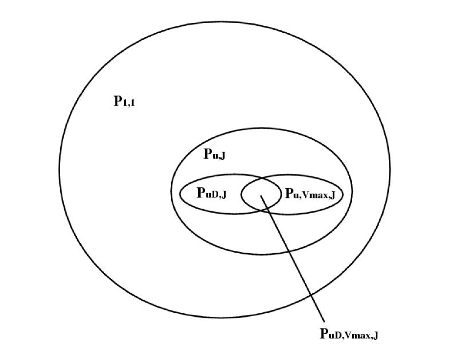
Figure 1: The relation between different classes of two enzyme pathways.

As an intuitive guide, the order of the generality of the representations discussed so far, in order of higher generality are: ${\bf P_{uD,V_{max},J}}\subset{\bf P_{uD,J}}\subset{\bf P_{u,J}}\subset{\bf P_{1,1}}$ and ${\bf P_{uD,V_{max},J}}\subset{\bf P_{u,V_{max},J}}\subset{\bf P_{u,J}}\subset{\bf P_{1,1}}$ (See Figure 1).

4.  Problems with the summation theroem

The definitions from the previous section have a series of logical implications. Here we present these implications and explain their significance. The proofs for these propositions are given in Appendix B.

4.1. Pathways with a constant input and a steady-state flux $({\bf P_{u,J}})$

Proposition 11

For any pathway of class ${\bf P_{u,J}}$, the flux summation theorem implies that for any given ratio of enzymes  $0\leq(E_{1}/E_{2})\leq\infty$ , there exists a $C_{\theta}$ such that flux is a linear function of the magnitude of the vector $\langle E_{1},E_{2}\rangle$.

$$\begin{array}[]{l}(\forall p\in{\bf P_{u,J}}):(\forall\theta~{}|~{}\tan\theta=E_{1}/E_{2}):(\exists C_{\theta}):\\ \left[~{}~{}C^{J}_{1}+C^{J}_{2}=1~{}~{}\Rightarrow~{}~{}J=\|\langle E_{1},E_{2}\rangle\|\,C_{\theta}~{}~{}\right].\end{array}$$ (11)

The meaning of proposition 11 is very simple. If a pathway were to be of class ${\bf P_{u,J}}$ and were to obey the flux summation theorem the following would hold: the flux would behave in a linear fashion with respect to tandem changes in which both enzyme concentrations are changed by the same percentage. It is a short few steps (Appendix B) to show that

$$\forall\left(\,\alpha=\frac{\delta E_{1}}{E_{1}}=\frac{\delta E_{2}}{E_{2}}\,\right):\,\,\left[\frac{\delta J}{J}=\alpha~{}\Leftrightarrow~{}J=\|\langle E_{1},E_{2}\rangle\|\,C_{\theta}\right].$$ (12)

Proposition (12) is equivalent to a statement of homogeneity ( See Giersch 1988 ), such that if $J=g[E_{1},E_{2}]$ then

$$g[~{}(1+\alpha)E_{1},\,(1+\alpha)E_{2}~{}]=(1+\alpha)g[~{}E_{1},\,E_{2}~{}].$$ (13)

For example consider two enzymes whose genes are located on the same operon. In addition consider the case in which such a cell is in a state in which the concentrations of the two enzymes are initially negligible. When the operon is turned on, each enzyme will have a particular rate of expression. If the ratio between those rates of expression remains constant, then the flux summation theorem would imply that the flux would increase linearly without reaching a saturation plateau. This is what $J=\|\langle E_{1},E_{2}\rangle\|\,C_{\theta}$ implies, where $\|\langle E_{1},E_{2}\rangle\|=\sqrt{E_{1}^{2}+E_{2}^{2}}$. Hence, in a pathway of class ${\bf P_{u,J}}$, in which we have made no assertion about the particulars of the enzyme-kinetic equations or parameters, the flux summation theorem assumes a particular type of dynamic behavior. A flux that increases linearly without saturation is a very special case and such a condition can only hold in a restricted subset of ${\bf P_{u,J}}$. In fact, as proposition 14 will attest, even for a simple pathway with the sole kinetic imposition of a diffusion barrier, the flux summation theorem fails.

4.2. Pathways with a diffusion barrier $({\bf P_{uD,J}})$

Proposition 14

For any pathway of class ${\bf P_{uD,J}}$, the flux summation theorem is false.

$$(\forall p\in{\bf P_{uD,J}}):\left[~{}~{}(\forall\delta E_{1},\,\delta E_{2}):~{}(\exists E_{1},E_{2}\in\mathbb{R}^{1}_{\geq 0}):~{}\left[~{}C^{J}_{1}+C^{J}_{2}\neq 1~{}\right]~{}~{}\right]$$ (14)

Proposition 14 basically states the general result that any pathway which has a diffusion barrier at a point before its first step will not obey the summation theorem. This includes almost any metabolic pathway that takes place in the confines of a cell. In fact it can be shown that any pathway that exhibits a plateauing effect on its flux surface will not obey the summation theorem. The proof of this theorem is intuitively simple (Appendix B). It is basically dependent on the conditional relation

$$C^{J}_{1}+C^{J}_{2}=1~{}~{}~{}\Rightarrow~{}~{}~{}J=\|\langle E_{1},E_{2}\rangle\|\,C_{\theta}$$ (15)

from (11). For any pathway class that is a subset of ${\bf P_{u,J}}$, if the pathways do not obey the right hand side of 15 then they do not obey the left hand side either. For ${\bf P_{uD,J}}$ one can show that $J=\|\langle E_{1},E_{2}\rangle\|\,C_{\theta}$ does not hold when $C_{\theta}>0$. This is because the diffusion barrier will impede flux from increasing indefinitley. This implies that $\sum_{i=1}^{n}C_{i}^{J}=1$ cannot be true for all enzyme concentrations. This falsehood applies to all diffusion-limited flux surfaces except for a disfunctional cell with flux surface $J=0$. Proposition 14 is due to the fact that control is not only dependent on the enzymatic steps in a pathway, but also the diffusion steps.

4.3. Pathways that allow for enzyme saturation $({\bf P_{u,V_{max},J}})$

Proposition 16

For any pathway of class ${\bf P_{u,V_{max},J}}$, if both enzymes approach saturation and changes in enzyme concentration are positive, then the sum of control coefficients approaches zero.

$$(\forall p\in{\bf P_{u,V_{max},J}}):\left[~{}(\forall\,\delta E_{1},\,\delta E_{2}\in\mathbb{R}^{1}_{>0}):~{}\underset{Sat_{1},Sat_{2}\rightarrow 1}{\lim}\left(C^{J}_{1}+C^{J}_{2}\right)=0~{}~{}\right].$$ (16)

Whenever two enzymes are near saturation, a situation is created whereupon the flux effects of increasing the concentration for one enzyme is restrained by the other enzyme. Hence whenever two enzymes approach saturation simultaneously, the sum of their control coefficients approaches zero and the flux summation theorem does not hold ( see appendix B ). In fact it is not too difficult to extend the proof such that for a sequential pathway of any length, the sum of all control coefficients will approach zero whenever any two enzymes approach saturation.

Proposition 17

For any pathway of class ${\bf P_{u,V_{max},J}}$ in which a decrease in enzyme concentration increases saturation, if both enzymes approach saturation and changes in enzyme concentration are negative, then the sum of control coefficients approaches two.  
 
For all intervals $a_{i}<E_{i}<b_{i}$:
If  $p\in{\bf P_{u,V_{max},J}}$  and $~{}\forall i$ : ( $\frac{\partial Sat_{i}}{E_{i}}\geq 0$   and   $a_{i}\geq 0$   and   $\delta E_{i}<0$  )    then:

$$\underset{Sat_{1},Sat_{2}\rightarrow 1}{\lim}{\left(C_{1}^{J}+C_{2}^{J}\right)=2}.$$ (17)

In such situations the pathway is no longer robust to decreases in enzyme concentration. Hence dominance is not an inherent property of these pathways. It is simple to extend this result to sequential pathways of any length, in which the sum of control coefficients will approach the the number of enzymes which are approaching saturation.

From propositions 14, 16 and 16 it also follows that the summation theorem is also false in pathways of class ${\bf P_{uD,V_{max},J}}$.

4.5. Enzyme interactions in ${\bf P_{u,J}}$

The motivation for analyzing multi-enzyme pathways is that they behave differently from single-enzymes. The natural question is to ask what are the direct or indirect interactions between enzymes that lead to the difference between single-enzyme and multi-enzyme pathway behavior. Interaction does not necessarily have to signify direct physical interaction between two enzymes. It can occur via the effect of one enzyme on the concentration of pathway intermediates that in turn physically interact with another enzyme. In equation (6) which was one of the assumptions that Kacser and Burns made in deriving the summation theorem, the proposition $\frac{\delta J}{J}=\sum_{i=1}^{n}\left(\frac{\delta J}{J}\right)_{i}$ amounts to an assumption that enzymes do not exhibit interactions. Here interaction is specifically referring to the mutual effect that the two enzymes would have on each-other’s ability to affect pathway flux:

Proposition 18

For any pathway of class ${\bf P_{u,J}}$, the proposition $\left[~{}\frac{\delta J}{J}=\sum_{i=1}^{n}\left(\frac{\delta J}{J}\right)_{i}~{}\right]$ (4) and the restriction $\left(\,\alpha=\frac{\delta E_{1}}{E_{1}}=\frac{\delta E_{2}}{E_{2}}\,\right)$ imply that the change in flux due to change of total enzyme concentration at one locus is independent of total enzyme concentration at the second locus in the pathway.

$$\begin{array}[]{l}(\forall p\in{\bf P_{u,J}}):(\forall E_{1},E_{2}\in\mathbb{R}^{1}_{\geq 0}):\\ \left[~{}~{}\left[~{}\forall\left(\,\alpha=\frac{\delta E_{1}}{E_{1}}=\frac{\delta E_{2}}{E_{2}}\,\right):~{}~{}\frac{\delta J}{J}=\sum_{i=1}^{2}\left(\frac{\delta J}{J}\right)_{i}\right]~{}~{}\Rightarrow~{}~{}\frac{\partial^{2}J}{\partial{E_{1}}\,\partial{E_{2}}}=0~{}~{}~{}\right].\end{array}$$ (18)

The assumption of independence of effects is something that surreptitiously goes against the motivation for developing MCA. Nonetheless the assumption of no enzyme interactions is built into the summation theorem from the beginning. In fact:

Proposition 19

For any pathway of class ${\bf P_{u,J}}$, the summation theorem implies that the change in flux due to change of total enzyme concentration at one locus is independent of total enzyme concentration at the second locus in the pathway.

$$\begin{array}[]{l}(\forall p\in{\bf P_{u,J}}):(\forall E_{1},E_{2}\in\mathbb{R}^{1}_{\geq 0}):\\ ~{}~{}~{}~{}~{}~{}~{}~{}~{}\left[~{}\left[(\forall\delta E_{1},\,\delta E_{2}):~{}C^{J}_{1}+C^{J}_{2}=1~{}\right]~{}~{}\Rightarrow~{}~{}\frac{\partial^{2}J}{\partial{E_{1}}\,\partial{E_{2}}}=0~{}~{}~{}\right].\end{array}$$ (19)

This means that the summation theorem implies the inexistence of epistasis. It immediately follows that

$$\begin{array}[]{l}(\forall p\in{\bf P_{uD,J}}):~{}\forall\left(E_{1},E_{2}\in\mathbb{R}^{1}_{\geq 0}~{}|~{}\frac{\partial^{2}J}{\partial{E_{1}}\,\partial{E_{2}}}\neq 0~{}\right):{}\\ ~{}~{}~{}~{}\left[~{}~{}(\exists\delta E_{1},\,\delta E_{2}):~{}\left[~{}C^{J}_{1}+C^{J}_{2}\neq 1~{}\right]~{}~{}\right].\end{array}$$ (20)

Hence in any regime where epistasis is present the summation theorem is violated. Furthermore:

Proposition 21

For any pathway of class ${\bf P_{u,J}}$, the summation theorem holds if and only if flux is a linear function of enzyme concentrations.

$$\begin{array}[]{l}(\forall p\in{\bf P_{u,J}}):(\forall E_{1},E_{2}\in\mathbb{R}^{1}_{\geq 0}):\\ ~{}~{}~{}~{}~{}~{}~{}~{}~{}\left[~{}\left[(\forall\delta E_{1},\,\delta E_{2}):~{}C^{J}_{1}+C^{J}_{2}=1~{}\right]~{}~{}\Leftrightarrow~{}~{}J=E_{1}\,c_{1}+E_{2}\,c_{2}~{}~{}~{}\right].\end{array}$$ (21)

In short, the summation theorem imposes conditions on enzyme interactions that are neither explicitly argued for nor conceptually justified.

5.  Numerical analysis of a pathway of class ${\bf P_{uD,V_{max},J}}$

Here we use numerical simulations for a particular case in order to verify the analytical results from the previous section. Consider a case where the enzymes exhibit reversible Michaelis-Menten kinetics. A diffusion barrier is included at the beginning of the pathway. During the interval of analysis $0\leq t\leq t_{f}$, the input remains constant such that $\dot{\bar{u}}(t)=0$ (e.g. approximation of large nutrient pool and/or steady state conditions of a chemostat). In such a case the full form of the system of differential equations (10) combined with the kinetic model (9) are:

$$\left(\begin{array}[]{l}\frac{\displaystyle d[s_{1}]}{\displaystyle dt}=-D\,{[s_{1}]}-{k1}\,{[e_{1}]}\,{[s_{1}]}+D\,[u]+{k2}\,{[\underline{es}_{1}]}\\ \\ \frac{\displaystyle d{[\underline{es}_{1}]}}{\displaystyle dt}={k1}\,{e_{1}}\,{[s_{1}]}-{k2}\,{[\underline{es}_{1}]}-{k3}\,{[\underline{es}_{1}]}+{k4}\,{[e_{1}]}\,{[s_{2}]}\\ \\ \frac{\displaystyle d[s_{2}]}{\displaystyle dt}={k3}\,{[\underline{es}_{1}]}-{k4}\,{[e_{1}]}\,{[s_{2}]}-{k5}\,{[e_{2}]}\,{[s_{2}]}+{k6}\,{[\underline{es}_{2}]}\\ \\ \frac{\displaystyle d[\underline{es}_{2}]}{\displaystyle dt}={k5}\,{[e_{2}]}\,{[s_{2}]}-{k6}\,{[\underline{es}_{2}]}-{k7}\,{[\underline{es}_{2}]}+{k8}\,{[e_{2}]}\,{[s_{3}]}\\ \\ \frac{\displaystyle d[s_{3}]}{\displaystyle dt}={k7}\,{[\underline{es}_{2}]}-Q\,{[s_{3}]}-{k8}\,{[e_{2}]}\,{[s_{3}]}\\ \\ \frac{\displaystyle d[e_{1}]}{\displaystyle dt}=-{k1}\,{[e_{1}]}\,{[s_{1}]}+{k2}\,{[\underline{es}_{1}]}+{k3}\,{[\underline{es}_{1}]}-{k4}\,{[e_{1}]}\,{[s_{2}]}\\ \\ \frac{\displaystyle d[e_{2}]}{\displaystyle dt}=-{k5}\,{[e_{2}]}\,{[s_{2}]}+{k6}\,{[\underline{es}_{2}]}+{k7}\,{[\underline{es}_{2}]}-{k8}\,{[e_{2}]}\,{[s_{3}]}\\ \\ \frac{\displaystyle d[o]}{\displaystyle dt}=Q\,{[s_{3}]}\\ \\ \end{array}\right)$$ (22)

where the postfix $(t)$ for each state variable is omitted.

The system of differential equations (22) will serve as the basis for the examination of a particular case. For the present analysis we are interested in the steady states of the dynamical system. At steady state, as defined in appendix A, the derivatives $\dot{{\bf s}}(t)\mbox{ and }\dot{{\bf e}}(t)$ are equal to zero. Consider a case where the equations in (22) serve as the basis for the functions $f_{1}$, $f_{2}$ and $f_{3}$ with the stoichiometric constraint that

$$\begin{array}[]{c}{[E_{1}]=[e_{1}]+[\underline{es}_{1}]}\\ {[E_{2}]=[e_{2}]+[\underline{es}_{2}]}.\end{array}$$ (23)

In such a case, the steady state solution can be obtained in an implicit form ( See appendix C ). The implicit equations can then be solved numerically by Newton-Raphson based algorithms that converge to the flux surface shown in Figure 2. On a cursory level the surface shows the plateau effect familiar in most models of two-enzyme pathways. The plateau arises due to the limiting effects of the diffusion barrier. We will refer to the pathway based on equations (22) as pathway $p_{\ref{odes}}$. It is not difficult to discern that pathway $p_{\ref{odes}}$ is a member of the set ${\bf P_{uD,V_{max},J}}$. It satisfies the conditions required in definitions 1 to 5.

5.1. Test of the summation theorem

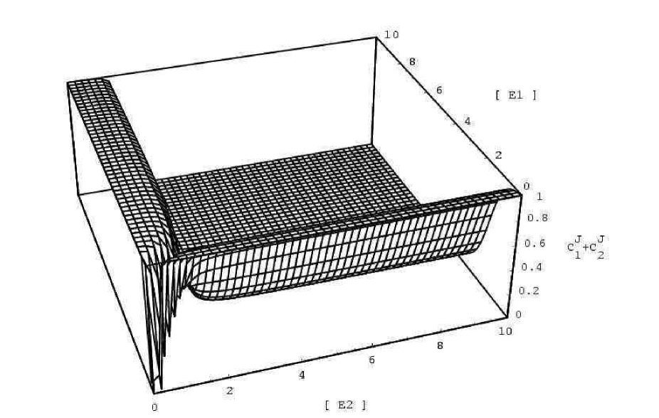
Figure 3: Sum of control coefficients as a function of total enzyme concentrations. Enzyme concentrations $[E_{i}]$ in $\mu M$. For both enzymes $\delta E_{i}=0.2\mu M$.

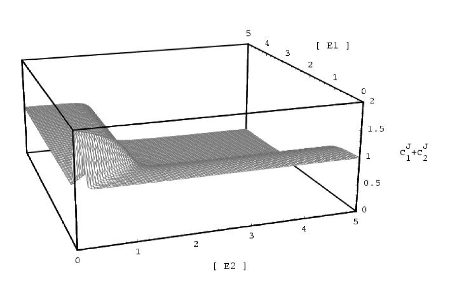
Figure 4: Sum of control coefficients as a function of total enzyme concentrations. Enzyme concentrations $[E_{i}]$ in $\mu M$. For both enzymes $\delta E_{i}=-0.2\mu M$.

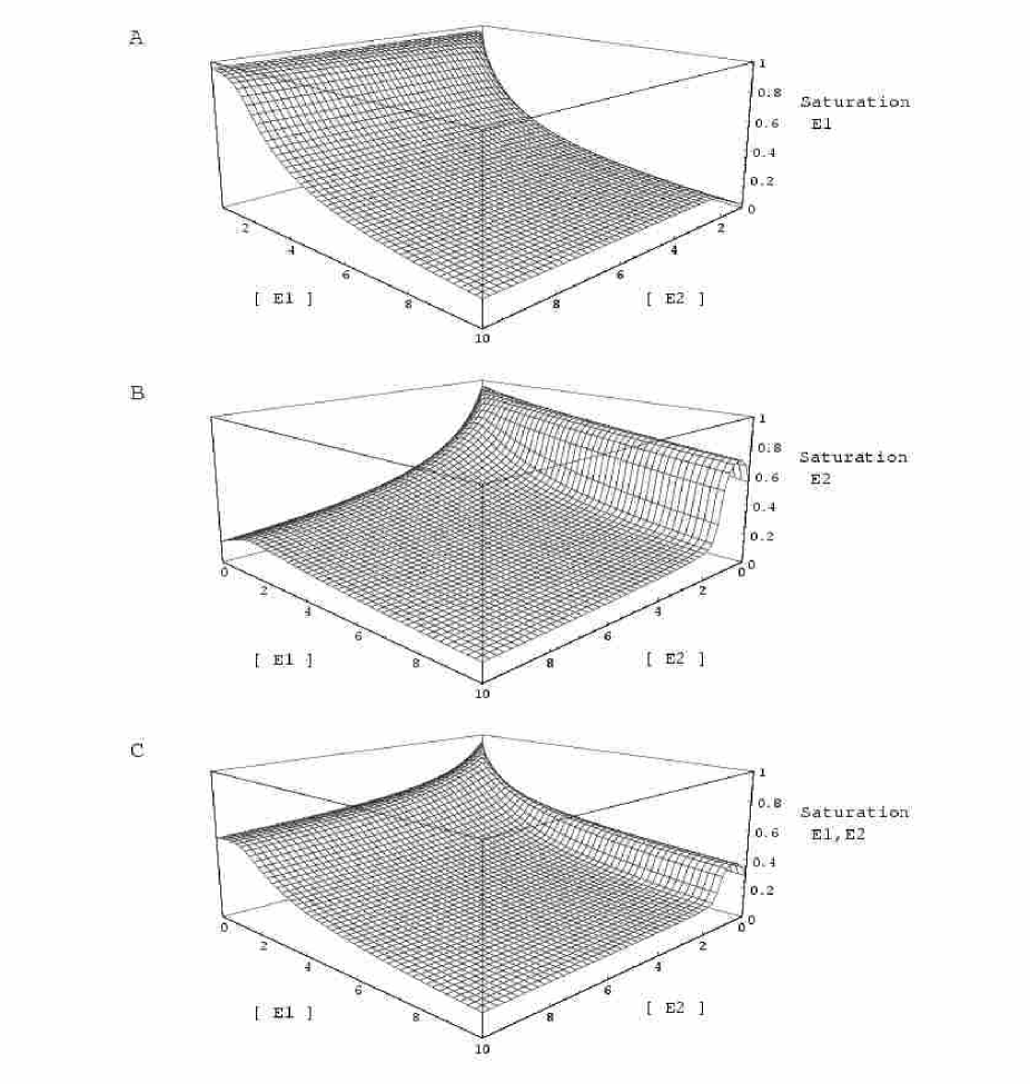
Figure 5: Enzyme saturation as a function of total enzyme concentrations. Single enzyme saturation is measured as $J/E_{i}k_{cat(i)}.$ Double enzyme saturation is measured as $(J/E_{1}k_{3}+J/E_{2}k_{7})/2.$ Enzyme concentrations $[E_{i}]$ in $\mu M$.

Given the flux surface on $p_{\ref{odes}}\in{\bf P_{uD,V_{max},J}}$, the flux summation theorem can be tested directly. Figures 3 and 4 show surfaces for for discrete versions of the sum $\sum_{i=1}^{n}C_{i}^{J}$ for $p_{\ref{odes}}$. It is evident from these examples that in the pathway $p_{\ref{odes}}$ there is no evidence of an invariant relation in which the control coefficients sum to the predetermined value of one. Figures 3 and 4 serve as illustrations of propositions 14, 16 and 17. The summation theorem fails in the regimes where flux is near its diffusion-limited maximal rate or in areas where both enzymes are near saturation. The regions where both enzymes approach saturation are shown in Figure 5.

5.2. Epistatic interactions between enzymes

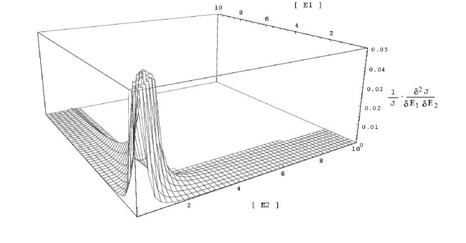
Figure 6: Measure of epistatic interaction effects on flux. Enzyme concentrations $[E_{i}]$ in $\mu M$. For both enzymes $\delta E_{i}=0.02\mu M$.

The question of the extent to which enzymes have interactive effects on flux can also be addressed directly using the pathway $p_{\ref{odes}}$ as an example. In Figure 6 the mixed partial difference ${\delta^{2}{J}}/{\delta{E_{1}}\delta{E_{2}}}$ is used as a measure of epistatic interactions between enzymes (proposition 18). Note that the region where the epistatic interactions increase coincides with a region where the summation theorem fails and both enzymes are approaching saturation.

5.3. Rate limiting enzymes and the switching of control between enzymes

One of the claims from MCA has been that there is no such thing as a rate limiting enzyme in a pathway. The associated claim is that control is mostly shared between enzymes in a pathway [Kacser, 1995]. The results of our numerical simulations of $p_{\ref{odes}}$ do not support this claim. Figure 7 shows the numerical results for two pathways with different $k_{cat}$ configurations. In the range of concentration regimes $\langle E_{1},E_{2}\rangle$ examined, most regimes manifest a sole enzyme as the controlling enzyme for a given pathway. In regimes where flux is near the diffusion limited maximal flux, no enzyme has control. The only region where the enzymes share control is where the summation theorem fails. In fact in the regions that the summation theorem holds, the sum $\sum_{i=1}^{2}C_{i}^{J}=1$ is basically the value $C^{J}_{z}$ for the sole controlling enzyme $z$ at that regime. Furthermore the identity of the controlling enzyme at a given regime is not invariant. The identity of the controlling enzyme can change by changing the $k_{cat}$ values of the enzymes involved (e.g. by mutation ). In Figure 7 the switch in control is clearly apparent by comparing the values of $C_{2}^{J}$ between the two $k_{cat}$ configurations.

6. Discussion and conclusion

The main intent of the present paper has been to present an analysis and critique of some of the main biological conclusions derived from MCA. Our results strongly support initial objections that were made with regards to the MCA perspective on the biochemical nature of dominance ( Cornish-Bowden 1987, Savageau 1992. See also Mayo & Burger 1997 ). At the core of the problem of multienzyme systems is interaction effects between enzymes. In order to address these interactions, the non-linear properties of enzyme catalysis cannot be ignored. These non-linear interactions play a major role in the phenotypic characteristics of metabolic physiology. Our analysis shows that for discrete changes of any magnitude, the flux summation theorem does not hold. This means that there are no a-priori constraints that would require the magnitude of mutational effects to be in a low range. This leaves open the possibility for two phenomena which had been previously rejected in MCA. In the first place, rate limiting steps or controlling enzymes do not have to be rare, and their identity can change by evolution. Secondly, phenotypic robustness with respect to mutations is not an automatic property of metabolic pathways; the degree of robustness can be modified through the evolution of kinetic properties. These are implications that we will examine in a later work.

Appendices

A.  Definitions

In this section some of the conditions proposed in definitions 1,2, 3 and 4 are formulated in a more precise language as definitions 2.2, 2.3, 2.4, 3.2 and 4.2. In these definitions quantifiers are encapsulated in parenthesis and propositions in square brackets. The symbol “$\wedge$” denotes the boolean expression “and”. The symbol “$\mathbb{R}^{1}_{\geq 0}$” denotes the real numbers greater than or equal to zero. Ordered tuples and vectors are encapsulated by the symbols “$\langle~{}\rangle$”. The property $K$ associated with an object $p$ is denoted as $(\mbox{``name of property"})\lfloor p\rfloor$.

Definition 1

$$\begin{array}[]{l}\\ (\forall p\in{\bf P_{1,1}}):\begin{array}[]{l}~{}p\Rightarrow\left[\begin{array}[]{l}{\dot{{\bf s}}(t)=f_{1}[{{\bf s}}(t),{{\bf e}}(t),u(t)]}~{}~{}\wedge\\ {\dot{{\bf e}}(t)=f_{2}[{{\bf s}}(t),{{\bf e}}(t)]}~{}~{}\wedge\\ {\dot{o}(t)=f_{3}[s_{3}(t)]}~{}\wedge{}\\ \left(u(t),o(t)\in\mathbb{R}^{1}_{\geq 0}\right)~{}\wedge~{}\left({\bf e}(0)\in\mathbb{R}^{4}_{\geq 0}\right)~{}\wedge~{}\left({\bf s}(0)\in\mathbb{R}^{3}_{\geq 0}\right)\end{array}\right]\\ \end{array}\end{array}$$ (24)

Definition 2.2

The proposition $(``\mbox{Stoichiometry: two enz. seq.}")\lfloor p\rfloor$ imposes both organizational and kinetic constraints on the pathway $p\in{\bf P_{u,J}}$ by designating the stoichiometric properties of the pathway. Such a proposition is necessary for an abstract representation of physical mass balance.

$$\begin{array}[]{l}(``\mbox{Stoichiometry: two enz. seq.}")\lfloor p\rfloor\equiv\\ ~{}~{}\begin{array}[]{l}(\,\forall(t,u(t),o(t))\in\mathbb{R}^{1}_{\geq 0}\,):(\forall{\bf e}(0)\in\mathbb{R}^{4}_{\geq 0}):(\forall{\bf s}(0)\in\mathbb{R}^{3}_{\geq 0}):\\ ~{}\left(\begin{array}[]{l}\left[\begin{array}[]{l}\begin{array}[]{l}{[~{}\dot{E}_{1}(t)=\dot{E}_{2}(t)=0~{}]}~{}~{}~{}~{}\wedge\\ {[~{}E_{1}=E_{1}(t)=e_{1}(t)+\underline{es}_{1}(t)~{}]}~{}~{}\wedge\\ {[~{}E_{2}=E_{2}(t)=e_{2}(t)+\underline{es}_{2}(t)~{}]}~{}~{}\wedge\\ {[~{}E_{1}\geq 0~{}\wedge~{}E_{2}\geq 0~{}]}\end{array}\end{array}\right]~{}~{}~{}~{}\wedge{}\\ \\ \left(\begin{array}[]{l}\left[\begin{array}[]{l}{\xi(t)=s_{1}(t)+2\underline{es}_{1}(t)+s_{2}(t)+2\underline{es}_{2}(t)}\\ {~{}~{}~{}~{}~{}~{}~{}~{}~{}~{}+s_{3}(t)+e_{1}(t)+e_{2}(t)}\end{array}\right]{~{}\wedge}{}\\ \\ \left(\begin{array}[]{l}(~{}\exists I_{in}(t),I_{rev}(t)\in\mathbb{R}^{1}_{\geq 0}~{}):\\ ~{}{[~{}~{}\dot{\xi}(t)=I_{in}(t)-I_{rev}(t)-\dot{o}(t)~{}~{}]}\end{array}\right)\end{array}\right)\end{array}\right)\end{array}\end{array}$$ (25)

where the pair $\langle E_{1},E_{2}\rangle\in\mathbb{R}^{2}_{\geq 0}$ are the total enzyme concentrations for any pathway $p$ such that $\langle E_{1},E_{2}\rangle$ does not change for each particular vector of starting conditions and that for a given set of initial conditions, the concentrations $E_{1}\mbox{ and }E_{2}$ are to be determined at any time $t$ by summing the free-enzyme and enzyme-substrate complex concentrations for each enzyme respectively. The variable $\xi(t)$ needs some explanation. $\xi(t)$ determines the “stoichiometric content” of the pathway in the sense that the coefficients $c_{i}$ in the equation

$${\xi(t)=c_{1}s_{1}(t)+c_{2}\underline{es}_{1}(t)+c_{3}s_{2}(t)+c_{4}\underline{es}_{2}(t)+c_{5}s_{3}(t)+c_{6}e_{1}(t)+c_{7}e_{2}(t)}$$

are determined by whether in reference to the input molecule, the transformations leading to the macro-molecules associated with each coefficient are fusions, cleavages or one-one transformations. The values of the $c_{i}$ in (25) correspond to the kinetic model (9). The equation for $\dot{\xi}(t)$ also deserves attention. Each metabolic pathway can be characterized such that $\dot{\xi}(t)$ is determined by the additive combination of two values at time $t$:

$$\dot{\xi}(t)=\mbox{\em Netstartflux(t) - Netendflux(t)}$$

which in turn can be subdivided as

$$\begin{array}[]{l}{\mbox{\em Netstartflux(t) = $I_{in}(t)-I_{rev}(t)$ \rm~{}~{}~{}~{}~{}~{}~{}~{}~{}~{}~{}~{}and}}\\ {\mbox{\em Netendflux(t) =$O_{out}(t)-O_{rev}(t)$}}\end{array}$$

where $I_{in}(t)$ is the flux entering the system from the input variable $u(t)$, $I_{rev}(t)$ is the flux exiting the system and going back into $u(t)$, $O_{out}(t)$ is the flux exiting the system into the output variable $o(t)$ and $O_{rev}(t)$ is the flux entering back into the system from $o(t)$. For a kinetic model with an irreversible sink step, $O_{rev}(t)=0$. For a system where the output variable ${o}(t)$ is only driven by a single pathway $p$, $O_{out}(t)=\dot{o}(t)$. Finally for ${\bf P_{u,J}}$ the only stipulations made for the two components of Netstartflux(t) is that they must both be greater or equal to zero such that $I_{in}(t),I_{rev}(t)\in\mathbb{R}^{1}_{\geq 0}$ and $\mbox{\em Netstartflux(t)}=I_{in}(t)-I_{rev}(t)$.

Definition 2.3

For a pathway $p\in{\bf P_{u,J}}$ the logical proposition
$(``\mbox{Const. u $\rightarrow$ Unique }\langle u,E_{1},E_{2},J^{*}\rangle")\lfloor p\rfloor$ states that given an input $u(t)$, if $u(t)$ remains constant then the pathway will reach a unique steady state flux $J^{*}\in\mathbb{R}^{1}_{\geq 0}$ that is dependent on total enzyme concentrations $E_{1}\mbox{ and }E_{2}$ such that:

$$\begin{array}[]{l}(``\mbox{Const. u $\rightarrow$ Unique }\langle u,E_{1},E_{2},J^{*}\rangle")\lfloor p\rfloor\equiv\\ ~{}(\,\forall u(0)\in\mathbb{R}^{1}_{\geq 0}\,):(\forall E_{1}(0),E_{2}(0)\in\mathbb{R}^{1}_{\geq 0}):\\ ~{}~{}(~{}\exists J^{*}\in\mathbb{R}^{1}_{\geq 0}~{}):(\,\forall o(t)\in\mathbb{R}^{1}_{\geq 0}\,):(\forall s_{1}(0),s_{2}(0),s_{3}(0)\in\mathbb{R}^{1}_{\geq 0}):\\ ~{}~{}~{}\left(\begin{array}[]{l}\left(\begin{array}[]{l}(\forall t\in\mathbb{R}^{1}_{\geq 0}):\\ ~{}~{}{[~{}\dot{u}(t)=0~{}]}\end{array}\right)~{}\Rightarrow~{}\left[\begin{array}[]{l}\underset{t\rightarrow\infty}{\lim}\dot{{\bf s}}(t)=\langle 0,0,0\rangle~{}\wedge{}\\ \underset{t\rightarrow\infty}{\lim}\dot{{\bf e}}(t)=\langle 0,0,0,0\rangle~{}\wedge{}\\ \underset{t\rightarrow\infty}{\lim}\ddot{o}(t)=0~{}\wedge{}\\ \underset{t\rightarrow\infty}{\lim}\dot{o}(t)=J^{*}\end{array}\right]\end{array}\right)\end{array}$$ (26)

Note that at steady state $\dot{\xi}(t)=0$.

Definition 2.4

The proposition $(``\mbox{computable: $\langle E_{1},E_{2},u\rangle\mapsto J~{}$}")\lfloor p\rfloor$ states that an approximation $J$ of $J^{*}$ is computable as a function of the initial input and total enzyme concentrations:

$$\begin{array}[]{l}{(``\mbox{computable: $\langle E_{1},E_{2},u\rangle\mapsto J~{}$}")\lfloor p\rfloor\equiv}\\ \left(\begin{array}[]{l}{(~{}\forall\varepsilon\in\mathbb{R}^{1}_{>0}~{}):(\exists g_{\varepsilon}:{\mathbb{R}^{3}_{\geq 0}\mapsto\mathbb{R}^{1}}):}\\ {(\,\forall(u(0),o(t))\in\mathbb{R}^{1}_{\geq 0}\,):(\forall{\bf e}(0)\in\mathbb{R}^{4}_{\geq 0}):(\forall{\bf s}(0)\in\mathbb{R}^{3}_{\geq 0}):}\\ \left(\begin{array}[]{l}~{}~{}{[~{}J=g_{\varepsilon}[u(0),E_{1},E_{2}]~{}\wedge~{}|J-J^{*}|\leq\varepsilon~{}]}\end{array}\right)\\ \end{array}\right)\end{array}$$ (27)

The above definition means that for any error margin $\varepsilon\geq 0$, there exists at-least one effectively computable function $g_{\varepsilon}$ that maps to the approximate value $J$ by using the total enzyme concentrations and initial input as arguments. Note that $g_{\varepsilon}$ as an effectively computable function refers to both numerical and analytic functions that can produce an approximation $J$. The assumption of computability is associated with the assumption that there is a rule based mechanistic relation between $E_{1}$, $E_{2}$ and $u$. There is a strong assumption inherent in the definitions of $g_{\varepsilon}$ in ${\bf P_{u,J}}$: that for any pathway $p\in{\bf P_{u,J}}$ a steady state flux exists and can be determined using only $u(0)$, $E_{1}$ and $E_{2}$ as arguments. That is, except for the constraints imposed by $u(0),E_{1}$ and $E_{2}$ the steady state is independent of the specifics of starting conditions. Note that for classes of pathways that exhibit multiple equilibria the trajectories become important and all the starting conditions have to be included as arguments in a newly defined computable function other than $g_{\varepsilon}$, which would be embedded in a system other than ${\bf P_{u,J}}$.

Definition 3.2

$$\begin{array}[]{l}(``\mbox{Diffusion Limited \em I}")\lfloor p\rfloor\equiv\\ ~{}~{}(\exists D\in\mathbb{R}^{1}_{\geq 0}):\\ ~{}~{}~{}~{}(\,\forall(t,u(t),o(t))\in\mathbb{R}^{1}_{\geq 0}\,):(\forall\bf{e}(0)\in\mathbb{R}^{4}_{\geq 0}):(\forall\bf{s}(0)\in\mathbb{R}^{3}_{\geq 0}):\\ ~{}~{}~{}~{}~{}\left(\begin{array}[]{l}{[~{}I_{in}(t)=D\,u(t)~{}]~{}~{}\wedge}{}{}\\ {[~{}I_{rev}(t)=D\,s_{1}(t)~{}]}\end{array}\right)\end{array}$$ (28)

where $D$ is the diffusion constant.

Definition 4.2

$$\begin{array}[]{l}(``\mbox{Saturable Enzymes}")\lfloor p\rfloor\equiv\\ ~{}~{}(\exists(k_{cat(1)},k_{cat(2)})\in\mathbb{R}^{1}_{\geq 0}):(\forall(E_{1},E_{2})\in\mathbb{R}^{1}_{\geq 0}):\\ ~{}~{}~{}~{}(\,\forall(t,u(t),o(t))\in\mathbb{R}^{1}_{\geq 0}\,):(\forall\bf{e}(0)\in\mathbb{R}^{4}_{\geq 0}):(\forall\bf{s}(0)\in\mathbb{R}^{3}_{\geq 0}):\\ ~{}~{}~{}~{}~{}\left(\begin{array}[]{l}{[~{}J\leq E_{1}k_{cat(1)}~{}]~{}~{}\wedge}{}{}\\ {[~{}J\leq E_{2}k_{cat(2)}~{}]}\end{array}\right)\end{array}$$ (29)

B.  Proofs

B.1  Proof of proposition 11

We start with the summation theorem $\sum_{i=1}^{n}C_{i}^{J}=1$. Using the definition of $C_{i}^{J}$ from (1) we have

$$(\forall E_{1},E_{2}\in\mathbb{R}^{1}_{>0}):~{}~{}~{}\frac{\delta{J}}{\delta{E_{1}}}\,\frac{E_{1}}{J}+\frac{\delta{J}}{\delta{E_{2}}}\,\frac{E_{2}}{J}=1.$$ (30)

The continuous version of (30) is $\underset{\delta E_{1},\,\delta E_{2}\rightarrow 0}{\lim}\left(\frac{\delta{J}}{\delta{E_{1}}}\,{E_{1}}+\frac{\delta{J}}{\delta{E_{2}}}\,{E_{2}}\right)=J$ which is equivalent to

$$\frac{\partial{J}}{\partial{E_{1}}}\,{E_{1}}+\frac{\partial{J}}{\partial{E_{2}}}\,{E_{2}}=J.$$ (31)

Equation (31) is a first order quasi-linear partial differential equation with general solution

$$J=E_{2}\,f\left[\frac{E_{1}}{E_{2}}\right]=E_{1}\,f^{\prime}\left[\frac{E_{2}}{E_{1}}\right],$$ (32)

where $f,f^{\prime}:\mathbb{R}^{1}\mapsto\mathbb{R}^{1}$ (see for example Rade & Westergren 1995, p230). For each fixed ratio of $E_{1}/E_{2}$, the vector $\langle E_{1},E_{2}\rangle$ forms a fixed angle $\theta$ with the coordinate axes $E_{2}$ and $E_{1}$ such that $E_{1}/E_{2}=\tan\theta$. Hence we can formulate the following proposition:

$$\begin{array}[]{c}(\exists g_{st}:{\mathbb{R}^{2}_{\geq 0}\mapsto\mathbb{R}^{1}}):(\forall E_{1},E_{2}\in\mathbb{R}^{1}_{>0}):(\exists f_{st}:{\mathbb{R}^{1}_{\geq 0}\mapsto\mathbb{R}^{1}}):\\ J~{}=~{}g_{st}[E_{1},E_{2}]~{}=~{}E_{2}\,f_{st}[\tan\theta]~{}=~{}h\,\cos\theta\,f_{st}[\tan\theta]\end{array}$$ (33)

where $h$ is the norm of the vector $\langle E_{1},E_{2}\rangle$ such that $h=\|\langle E_{1},E_{2}\rangle\|=\sqrt{E_{1}^{2}+E_{2}^{2}}\,$. Given that for every $\theta$ there exists a $C_{\theta}$ such that $C_{\theta}=\cos\theta\,\cdot f_{st}[\tan\theta]$, we have

$$(\forall\theta\mid 0\leq\theta\leq{\pi}/{2}):(\exists C_{\theta}):[~{}J=h\,C_{\theta}~{}].$$ (34)

$~{}~{}~{}~{}~{}~{}~{}~{}~{}~{}~{}~{}~{}~{}~{}~{}~{}~{}~{}~{}~{}~{}~{}~{}~{}~{}~{}~{}~{}~{}~{}~{}~{}~{}~{}~{}~{}~{}~{}~{}~{}~{}~{}~{}~{}~{}~{}~{}~{}~{}~{}~{}~{}~{}~{}~{}~{}~{}~{}~{}~{}~{}~{}~{}~{}~{}~{}~{}~{}~{}~{}~{}~{}~{}~{}~{}~{}~{}~{}~{}\blacksquare{\bf~{}proposition~{}{\ref{theorem1}}}$

B.2  Proof of Proposition 12

The proof of the proposition $\left[\frac{\delta J}{J}=\alpha~{}~{}\Leftrightarrow~{}~{}J=\|\langle E_{1},E_{2}\rangle\|\,C_{\theta}\right]$ is uncomplicated. We start with proving the forward conditional $\left[\frac{\delta J}{J}=\alpha~{}~{}\Rightarrow~{}~{}J=\|\langle E_{1},E_{2}\rangle\|\,C_{\theta}\right]$. By definition we are given that

$$\alpha=\delta E_{1}/E_{1}=\delta E_{2}/E_{2}.$$ (35)

Consider the vector $\langle E_{1},E_{2}\rangle$ and its norm $h=\|\langle E_{1},E_{2}\rangle\|=\sqrt{E_{1}^{2}+E_{2}^{2}}\,$. Given simultaneous increases in enzyme concentration $\delta E_{1}$ and $\delta E_{2}$ that obey (35) we have $h+\delta h=\sqrt{(1+\alpha)^{2}E_{1}^{2}+(1+\alpha)^{2}E_{2}^{2}}$. Hence $\delta h/h=\alpha$ and thereby

$$\delta J/J=\delta h/h.$$ (36)

In its continuous form equation (36) can be set up as a separable differential equation such that

$$(\forall~{}{E_{1}}/{E_{2}}):\left[\frac{dJ}{J}=\frac{dh}{h}\right].$$ (37)

Integrating both sides of (37) we have the solution

$$(\forall~{}E_{1}/E_{2}):(\exists C_{\theta}):\left[J=h\,C_{\theta}\right].$$ (38)

The backward conditional $\left[\frac{\delta J}{J}=\alpha~{}~{}\Leftarrow~{}~{}J=\|\langle E_{1},E_{2}\rangle\|\,C_{\theta}\right]$ can be proven by differentiating (38) with respect to $h$.

$~{}~{}~{}~{}~{}~{}~{}~{}~{}~{}~{}~{}~{}~{}~{}~{}~{}~{}~{}~{}~{}~{}~{}~{}~{}~{}~{}~{}~{}~{}~{}~{}~{}~{}~{}~{}~{}~{}~{}~{}~{}~{}~{}~{}~{}~{}~{}~{}~{}~{}~{}~{}~{}~{}~{}~{}~{}~{}~{}~{}~{}~{}~{}~{}~{}~{}~{}~{}~{}~{}~{}~{}~{}~{}~{}~{}~{}~{}~{}~{}~{}~{}~{}~{}~{}\blacksquare{\bf~{}Proposition~{}\ref{linequiv}}$

B.3  Proof of proposition 14

Consider a case where we posit the existence of a pathway $p_{1}\in{\bf P_{u,J}}$ which obeys the flux summation theorem . In such a case, using (34) we have;

$$\begin{array}[]{l}(\forall\theta\mid 0\leq\theta\leq{\pi}/{2}):\\ {[~{}[~{}h\rightarrow\infty~{}]~{}\Leftrightarrow~{}[~{}E_{1}\rightarrow\infty~{}\wedge~{}E_{2}\rightarrow\infty~{}]~{}]}.\end{array}$$ (39)

Furthermore for the function $g_{st}$ defined in (33) we have the following implication:

$$\begin{array}[]{l}\left((\exists p_{1}\in{\bf P_{u,J}}):\left[(\forall E_{1},E_{2}\in\mathbb{R}^{1}_{>0}):\sum_{i=1}^{n}C_{i}^{J}=1\right]\right):(\forall E_{1},E_{2}\in\mathbb{R}^{1}_{\geq 0}):\\ \underset{h\rightarrow\infty}{\lim}\,J=\underset{h\rightarrow\infty}{\lim}\,g_{st}[E_{1},E_{2}]=\underset{h\rightarrow\infty}{\lim}\,h\cdot\cos c_{1}\cdot f_{st}[\tan c_{1}]=\underset{h\rightarrow\infty}{\lim}\,h\,C_{\theta}=\infty.\end{array}$$ (40)

On the other hand consider a diffusion-limited pathway $p_{2}\in{\bf P_{uD,J}}$ where $J=g[E_{1},E_{2}]$ as defined by (61). When the system reaches a steady state as defined by (26), we know by (25) that $\dot{\xi}(t)=0$ and $0=I_{in}(t)-I_{rev}(t)-\dot{o}(t)$. Since $\underset{t\rightarrow\infty}{\lim}\dot{o}(t)=J^{*}$, using (28) we have the steady state condition:

$$\begin{array}[]{l}{J^{*}=D\,u(t)-D\,s_{1}(t)\mbox{~{}~{}~{}~{}and}}\\ {J\pm\varepsilon=D\,u(t)-Ds_{1}(t)}.\end{array}$$

Since $\dot{u}(t)=0$;

$$\ \begin{array}[]{l}{(\forall p_{2}\in{\bf P_{uD,J}}):(\exists D):(\forall u(0)=c_{2}):(\forall\varepsilon):}\\ {[~{}c_{3}=D\,c_{2}~{}]~{}\wedge~{}[~{}J\pm\varepsilon=c_{3}-Ds_{1}(t)~{}]}.\end{array}$$ (41)

Recall that $D\geq 0$ by (28) and $s_{1}(t)\geq 0$ by (24). For any finite $0<\varepsilon<\infty$ we can define a constant $c_{4}$ such that $c_{4}=c_{3}+\varepsilon$. Consequently

$$J\leq c_{4}$$ (42)

where we know that $0<c_{4}<\infty$. Hence

$$\begin{array}[]{l}(\forall p_{2}\in{\bf P_{uD,J}}):(\forall(E_{1},E_{2})\in\mathbb{R}^{1}_{>0}:\\ \underset{h\rightarrow\infty}{\lim}\,J=\underset{h\rightarrow\infty}{\lim}\,g[E_{1},E_{2}]\leq(c_{4}<\infty).\end{array}$$ (43)

If we now posit a pathway $p_{3}$ that both obeys the flux summation theorem and is diffusion-limited, propositions (40) and (43) lead to the proposition:

$$\begin{array}[]{l}\exists(p_{3}\in{\bf P_{uD,J}}):\left(\begin{array}[]{l}{[~{}p_{3}\in{\bf P_{u,J}}~{}]~{}\wedge~{}\left[(\forall E_{1},E_{2}\in\mathbb{R}^{1}_{\geq 0}):\sum_{i=1}^{n}C_{i}^{J}=1\right]}~{}\wedge{}\\ {~{}~{}~{}~{}~{}~{}~{}~{}~{}~{}~{}~{}~{}~{}~{}~{}~{}~{}~{}~{}~{}[~{}\infty\leq(c_{4}<\infty)~{}]}\end{array}\right)\end{array}$$ (44)

which is a contradiction. Therefore

$$(\forall p\in{\bf P_{uD,J}}):\left[~{}~{}\neg\left[(\forall E_{1},E_{2}\in\mathbb{R}^{1}_{\geq 0}):~{}\sum_{i=1}^{n}C_{i}^{J}=1~{}\right]~{}~{}\right].$$

$~{}~{}~{}~{}~{}~{}~{}~{}~{}~{}~{}~{}~{}~{}~{}~{}~{}~{}~{}~{}~{}~{}~{}~{}~{}~{}~{}~{}~{}~{}~{}~{}~{}~{}~{}~{}~{}~{}~{}~{}~{}~{}~{}~{}~{}~{}~{}~{}~{}~{}~{}~{}~{}~{}~{}~{}~{}~{}~{}~{}~{}~{}~{}~{}~{}~{}~{}~{}~{}~{}~{}~{}~{}~{}~{}~{}~{}~{}~{}\blacksquare{\bf~{}proposition~{}\ref{theorem2}}$

B.4  Proof of proposition 16

For a pathway $p\in{\bf P_{u,V_{max},J}}$, consider a case in which enzyme 2 is saturable such that

$$(\forall E_{1}\in\mathbb{R}^{1}_{>0}):~{}~{}~{}\left[~{}J\leq E_{2}k_{cat(2)}~{}~{}~{}\wedge~{}~{}~{}J^{\prime}\leq E_{2}k_{cat(2)}~{}\right],$$ (45)

where for any $\delta E_{1}$, $J^{\prime}=J+\delta J$. It follows that if $E_{2}$ is held constant, for any $\delta E_{1}$

$$\frac{\delta J}{\delta E_{1}}\leq\frac{E_{2}k_{cat(2)}-J}{\delta E_{1}}.$$ (46)

Multiplying both sides by $E_{1}/J$ we have

$$\frac{E_{1}}{J}\,\frac{\delta J}{\delta E_{1}}\leq\frac{E_{1}E_{2}k_{cat(2)}-JE_{1}}{J\delta E_{1}}.$$ (47)

Hence by (1) we obtain

$$C_{1}^{J}\leq~{}\frac{E_{1}E_{2}k_{cat(2)}}{J\delta E_{1}}-\frac{E_{1}}{\delta E_{1}}.$$ (48)

In a similar fashion if enzyme 1 is saturable and $E_{1}$ held constant, for any $\delta E_{2}$ we have

$$C_{2}^{J}\leq~{}\frac{E_{1}E_{2}k_{cat(1)}}{J\delta E_{2}}-\frac{E_{2}}{\delta E_{2}}.$$ (49)

For each enzyme $i$, consider a measure of saturation $Sat_{i}$ such that

$$Sat_{i}={J}/{E_{i}k_{cat(i)}}.$$ (50)

It follows that for any enzyme $i$,

$$\underset{Sat_{i}\rightarrow 1}{\lim}{\left(\frac{E_{i}k_{cat(i)}}{J}\right)=1}.$$ (51)

Denoting $R.H.S.(\ref{ineqcij1})$ as the right hand side of (48), as enzyme 2 approaches saturation, (51) and (48) imply that

$$\underset{Sat_{2}\rightarrow 1}{\lim}\left(R.H.S.(\ref{ineqcij1})\right)=\frac{E_{1}}{\delta E_{1}}-\frac{E_{1}}{\delta E_{1}}=0.$$ (52)

Similarly, if enzyme 1 is approaching saturation, (51) and (49) imply that

$$\underset{Sat_{2}\rightarrow 1}{\lim}\left(R.H.S.(\ref{ineqcij2})\right)=\frac{E_{2}}{\delta E_{2}}-\frac{E_{2}}{\delta E_{2}}=0.$$ (53)

Consequently when both enzyme 1 and enzyme 2 approach saturation, (52) and (53) imply that

$$(\forall p\in{\bf P_{u,V_{max},J}}):\left[~{}(\forall\delta E_{1},\,\delta E_{2}\in\mathbb{R}^{1}_{>0}):~{}\underset{Sat_{1},Sat_{2}\rightarrow 1}{\lim}\left({\sum_{i=1}^{2}}C_{i}^{J}\right)=0~{}~{}\right].$$ (54)

$~{}~{}~{}~{}~{}~{}~{}~{}~{}~{}~{}~{}~{}~{}~{}~{}~{}~{}~{}~{}~{}~{}~{}~{}~{}~{}~{}~{}~{}~{}~{}~{}~{}~{}~{}~{}~{}~{}~{}~{}~{}~{}~{}~{}~{}~{}~{}~{}~{}~{}~{}~{}~{}~{}~{}~{}~{}~{}~{}~{}~{}~{}~{}~{}~{}~{}~{}~{}~{}~{}~{}~{}~{}~{}~{}~{}~{}~{}~{}~{}~{}\blacksquare{\bf~{}proposition~{}\ref{theorem4}}$

B.4  Proof of proposition 17

For a pathway $p\in{\bf P_{u,V_{max},J}}$, consider a case in which enzyme 2 is saturable such that

$$(\forall E_{1}\in\mathbb{R}^{1}_{>0}):~{}~{}~{}\left[~{}J\leq E_{2}k_{cat(2)}~{}~{}~{}\wedge~{}~{}~{}J^{\prime}\leq E_{2}k_{cat(2)}~{}\right],$$ (55)

where for any $\delta E_{2}$, $J^{\prime}=J+\delta J$.

Given that $Sat_{i}={J}/{E_{i}k_{cat(i)}},$ if $E_{1}$ is held constant, for any $\delta E_{2}<0$ then

$$\underset{Sat_{2}\rightarrow 1}{\lim}{\left(\frac{E_{2}k_{cat(2)}}{J}\right)=1}\mbox{ ~{}~{}~{} and~{}~{}~{} }\underset{Sat_{2}\rightarrow 1}{\lim}{\left(J\right)=E_{2}k_{cat(2)}}.$$ (56)

Given (55) and (56), for domains in which decreasing $E_{2}$ increases saturation we have:
For all intervals $a<E_{2}<b$ :
If $\frac{\partial Sat_{2}}{E_{2}}\geq 0$   and   $a\geq 0$   and   $\delta E_{2}<0$   then:

$$\underset{Sat_{2}\rightarrow 1}{\lim}{\left(\delta J\right)=\delta E_{2}k_{cat(2)}}.$$ (57)

Hence

$$\underset{Sat_{2}\rightarrow 1}{\lim}{\left(C_{2}^{J}\right)}=\underset{Sat_{2}\rightarrow 1}{\lim}{\left(\frac{\delta J/J}{\delta E/E}\right)}=\frac{\delta E_{2}k_{cat(2)}/k_{cat(2)}}{\delta E_{2}/E_{2}}=1.$$ (58)

Similarly if enzyme 1 is saturable we can show that

$$\underset{Sat_{1}\rightarrow 1}{\lim}{\left(C_{1}^{J}\right)}=1.$$ (59)

Hence for all intervals $a_{i}<E_{i}<b_{i}$ :

$$\begin{array}[]{l}(\forall p\in{\bf P_{u,V_{max},J}}):\\ \left(\begin{array}[]{l}\left[~{}\forall i:\left(~{}\frac{\partial Sat_{i}}{E_{i}}\geq 0~{}~{}~{}\wedge~{}~{}~{}a_{i}\geq 0~{}~{}~{}\wedge~{}~{}~{}\delta E_{i}<0~{}\right)~{}\right]\Rightarrow\\ ~{}~{}~{}~{}~{}~{}~{}~{}~{}~{}~{}~{}\underset{Sat_{1},Sat_{2}\rightarrow 1}{\lim}{\left(C_{1}^{J}+C_{2}^{J}\right)=2}\end{array}\right)\end{array}$$ (60)

$~{}~{}~{}~{}~{}~{}~{}~{}~{}~{}~{}~{}~{}~{}~{}~{}~{}~{}~{}~{}~{}~{}~{}~{}~{}~{}~{}~{}~{}~{}~{}~{}~{}~{}~{}~{}~{}~{}~{}~{}~{}~{}~{}~{}~{}~{}~{}~{}~{}~{}~{}~{}~{}~{}~{}~{}~{}~{}~{}~{}~{}~{}~{}~{}~{}~{}~{}~{}~{}~{}~{}~{}~{}~{}~{}~{}~{}~{}~{}~{}~{}\blacksquare{\bf~{}proposition~{}\ref{theorem4_2}}$

B.5  Proof of proposition 18

The most straight forward proof of (18) is by direct deduction. To do this we define a set of notations for representing discrete changes in steady state flux due to changes in enzyme concentration.

Definition B.4a:

For a given input $u(t)$ that is constant, let $J$ be the abbreviated notation for the result of a mapping in a function $g:\mathbb{R}^{2}\mapsto\mathbb{R}^{1}$, with the variables $E_{1}$ and $E_{2}$ as arguments:

$$\begin{array}[]{l}(\forall p\in{\bf P_{u,J}}):\\ {(\forall u(0)\in\mathbb{R}^{1}):(\forall(\varepsilon>0)\in\mathbb{R}^{1}_{\geq 0}):(\exists g:{\mathbb{R}^{2}_{\geq 0}\mapsto\mathbb{R}^{1}}):}\\ {[~{}~{}J=g[E_{1},E_{2}]~{}~{}~{}\Leftrightarrow~{}~{}~{}J=g_{\varepsilon}[u(0),E_{1},E_{2}]~{}~{}]}\end{array}$$ (61)

The discrete operator $(~{})\stackrel{{\scriptstyle E_{1}E_{2}}}{{\longmapsto}}$ applied to $J$ is defined as:

$$J\stackrel{{\scriptstyle{E_{1}}{E_{2}}}}{{\longmapsto}}\,\equiv~{}g[E_{1}+\delta E_{1}~{},~{}E_{2}+\delta E_{2}]$$

where the symbol “$\equiv$” denotes identity by definition and for a given function $g$, the increments in $E_{1}$ and $E_{2}$ are held constant such that $\delta E_{1}=c_{1}$,  $\delta E_{2}=c_{2}$ and $c_{1},c_{2}\in\mathbb{R}^{1}_{\geq 0}$. Similarly,

$$J\stackrel{{\scriptstyle{E_{1}}{\,}}}{{\longmapsto}}\,\equiv\,g[E_{1}+\delta E_{1}~{},~{}E_{2}]\mbox{~{}~{}~{}~{}and~{}~{}~{}~{}}J\stackrel{{\scriptstyle{\,}{E_{2}}}}{{\longmapsto}}\,\equiv\,g[E_{1}~{},~{}E_{2}+\delta E_{2}].$$

Note that the operator $(~{})\stackrel{{\scriptstyle{(~{})}{\,}}}{{\longmapsto}}$ can be applied iteratively and is also commutative in its iteration order such that

$$(J\stackrel{{\scriptstyle{E_{1}}{\,}}}{{\longmapsto}})\stackrel{{\scriptstyle{\,}{E_{2}}}}{{\longmapsto}}~{}~{}=~{}~{}J\stackrel{{\scriptstyle{E_{1}}{E_{2}}}}{{\longmapsto}}~{}~{}=~{}~{}(J\stackrel{{\scriptstyle{\,}{E_{2}}}}{{\longmapsto}})\stackrel{{\scriptstyle{E_{1}}{\,}}}{{\longmapsto}}$$

Definition B.5b:

Let the operator $(~{})\overset{(~{})}{\underset{\Delta}{(\longmapsto)}}$ applied to $J\stackrel{{\scriptstyle{E_{1}}{E_{2}}}}{{\longmapsto}}$ be defined as

$$J\overset{{E_{1}}{E_{2}}}{\underset{\Delta}{\longmapsto}}\,\equiv\,J\stackrel{{\scriptstyle{E_{1}}{E_{2}}}}{{\longmapsto}}-J$$

where from Definition A1 we get $(J\stackrel{{\scriptstyle{E_{1}}{E_{2}}}}{{\longmapsto}}-J)=(g[E_{1}+\delta E_{1},E_{2}+\delta E_{2}]-g[E_{1},E_{2}])$. Similarly,

$$J\overset{{E_{1}}{\,}}{\underset{\Delta}{\longmapsto}}\,\equiv\,J\stackrel{{\scriptstyle{E_{1}}{\,}}}{{\longmapsto}}-J\mbox{~{}~{}~{}~{}and~{}~{}~{}~{}}J\overset{{\,}{E_{2}}}{\underset{\Delta}{\longmapsto}}\,\equiv\,J\stackrel{{\scriptstyle{E_{2}}{\,}}}{{\longmapsto}}-J.$$

Proof Argument:

To prove the relation

$$\begin{array}[]{l}(\forall E_{1},E_{2}\in\mathbb{R}^{1}_{\geq 0}):\\ \left[~{}~{}\forall\left(\,\alpha=\frac{\delta E_{1}}{E_{1}}=\frac{\delta E_{2}}{E_{2}}\,\right):~{}~{}\frac{\delta J}{J}=\sum_{i=1}^{n}\left(\frac{\delta J}{J}\right)_{i}~{}~{}\right]~{}~{}\Rightarrow~{}~{}\frac{\partial^{2}J}{\partial{E_{1}}\,\partial{E_{2}}}=0,\end{array}$$ (62)

we start with the left hand side of the relation, which is equation (4) from the Kacser & Burns derivation. Using definitions B.5a and B.5b for a two enzyme pathway, equation (4) is equivalent to

$$\frac{J\overset{{E_{1}}{E_{2}}}{\underset{\Delta}{\longmapsto}}\,}{J}=\frac{J\overset{{E_{1}}{\,}}{\underset{\Delta}{\longmapsto}}}{J}+\frac{J\overset{{\,}{E_{2}}}{\underset{\Delta}{\longmapsto}}}{J}.$$ (63)

By cancelling the denominator in (63) we proceed with a series of deductions in which the horizontal symbol “$\Updownarrow$” denotes the biconditional relation “ if and only if ” between successive lines. The explanation for each biconditional is given to its right:

$$(\forall E_{1},E_{2}\in\mathbb{R}^{1}_{\geq 0}):~{}\forall\left(\,\alpha=\frac{\delta E_{1}}{E_{1}}=\frac{\delta E_{2}}{E_{2}}\,\right):$$

$$J\overset{{E_{1}}{E_{2}}}{\underset{\Delta}{\longmapsto}}\, =J\overset{{E_{1}}{\,}}{\underset{\Delta}{\longmapsto}}+J\overset{{\,}{E_{2}}}{\underset{\Delta}{\longmapsto}}$$

$$\Updownarrow\mbox{~{}using~{} Definitions~{} B.5a~{} \&~{} B.5b}$$

$$g[E_{1}+\delta E_{1}~{},~{}E_{2}+\delta E_{2}]-g[E_{1},E_{2}] =(g[E_{1}+\delta E_{1}~{},~{}E_{2}]-g[E_{1},E_{2}])$$

$$~{}~{}~{}~{}~{}+(g[E_{1}~{},~{}E_{2}+\delta E_{2}]-g[E_{1},E_{2}])$$

$$\Updownarrow\mbox{rearrange}$$

$$(g[E_{1}+\delta E_{1}~{},~{}E_{2}+\delta E_{2}]-g[E_{1}+\delta E_{1}~{},~{}E_{2}]) -(g[E_{1}~{},~{}E_{2}+\delta E_{2}]-g[E_{1},E_{2}])=0$$

$$\Updownarrow\mbox{~{}using~{} Definitions~{} B.5a~{} \&~{} B.5b}$$

$$(g[E_{1}~{},~{}E_{2}+\delta E_{2}]-g[E_{1},E_{2}])\overset{{E_{1}}{\,}}{\underset{\Delta}{\longmapsto}}~{} =0$$

$$\Updownarrow\mbox{~{}using~{} Definitions~{} B.5a~{} \&~{} B.5b}$$

$$(\forall E_{1},E_{2}\in\mathbb{R}^{1}_{\geq 0}):~{}\forall\left(\,\alpha=\frac{\delta E_{1}}{E_{1}}=\frac{\delta E_{2}}{E_{2}}\,\right):$$

$$((J)\overset{{\,}{E_{2}}}{\underset{\Delta}{\longmapsto}})\overset{{E_{1}}{\,}}{\underset{\Delta}{\longmapsto}} =0.$$

Hence

$$\begin{array}[]{l}(\forall E_{1},E_{2}\in\mathbb{R}^{1}_{\geq 0}):~{}\forall\left(\,\alpha=\frac{\delta E_{1}}{E_{1}}=\frac{\delta E_{2}}{E_{2}}\,\right):\\ ~{}~{}\left[\frac{\delta J}{J}=\sum_{i=1}^{n}\left(\frac{\delta J}{J}\right)_{i}~{}~{}\Leftrightarrow~{}~{}((J)\overset{{\,}{E_{2}}}{\underset{\Delta}{\longmapsto}})\overset{{E_{1}}{\,}}{\underset{\Delta}{\longmapsto}}=0~{}~{}\right].\end{array}$$ (64)

The proposition $((J)\overset{{\,}{E_{2}}}{\underset{\Delta}{\longmapsto}})\overset{{E_{1}}{\,}}{\underset{\Delta}{\longmapsto}}=0$  is operationally equivalent to the sentence in proposition 14 that proposes the independence of control effects. Next it is simple to show equivalence to a continuous version such that

$$\begin{array}[]{l}(\forall E_{1},E_{2}\in\mathbb{R}^{1}_{\geq 0}):\\ \left[~{}\left[~{}\forall\left(\,\alpha=\frac{\delta E_{1}}{E_{1}}=\frac{\delta E_{2}}{E_{2}}\,\right):~{}((J)\overset{{\,}{E_{2}}}{\underset{\Delta}{\longmapsto}})\overset{{E_{1}}{\,}}{\underset{\Delta}{\longmapsto}}=0~{}\right]~{}~{}\Rightarrow~{}~{}\frac{\partial^{2}J}{\partial{E_{1}}\,\partial{E_{2}}}=0~{}~{}\right].\end{array}$$ (65)

From the third line of our sequence of biconditional relations we know that the left hand side of (65) has to comply with the equivalence

$$\begin{array}[]{l}(\forall E_{1},E_{2}\in\mathbb{R}^{1}_{\geq 0}):~{}\forall\left(\,\alpha=\frac{\delta E_{1}}{E_{1}}=\frac{\delta E_{2}}{E_{2}}\,\right):\\ \left[~{}~{}((J)\overset{{\,}{E_{2}}}{\underset{\Delta}{\longmapsto}})\overset{{E_{1}}{\,}}{\underset{\Delta}{\longmapsto}}=0~{}~{}\Leftrightarrow~{}~{}J\stackrel{{\scriptstyle{E_{1}}{E_{2}}}}{{\longmapsto}}-J\stackrel{{\scriptstyle{E_{1}}{\,}}}{{\longmapsto}}-J\stackrel{{\scriptstyle{\,}{E_{2}}}}{{\longmapsto}}+J=0~{}~{}\right].\end{array}$$ (66)

We also know by the general definition of partial differentiation that

$$\frac{\partial{J}}{\partial{E_{1}}}=\underset{\delta E_{1}\rightarrow 0}{\lim}\left(\frac{J\stackrel{{\scriptstyle{E_{1}}{\,}}}{{\longmapsto}}-J}{\delta E_{1}}\right)~{}~{}~{}~{}\mbox{ and }$$

$$\frac{\partial^{2}{J}}{\partial{E_{1}}\partial{E_{2}}}=\underset{\delta E_{1},\,\delta E_{2}\rightarrow 0}{\lim}\left(~{}\frac{J\stackrel{{\scriptstyle{E_{1}}{E_{2}}}}{{\longmapsto}}-J\stackrel{{\scriptstyle{E_{1}}{\,}}}{{\longmapsto}}-J\stackrel{{\scriptstyle{\,}{E_{2}}}}{{\longmapsto}}+J}{\delta E_{1}\,\delta E_{2}}~{}\right).$$ (67)

Substituting (66) into (67) we get (65). Using (65) and (64) we get (62).
$~{}~{}~{}~{}~{}~{}~{}~{}~{}~{}~{}~{}~{}~{}~{}~{}~{}~{}~{}~{}~{}~{}~{}~{}~{}~{}~{}~{}~{}~{}~{}~{}~{}~{}~{}~{}~{}~{}~{}~{}~{}~{}~{}~{}~{}~{}~{}~{}~{}~{}~{}~{}~{}~{}~{}~{}~{}~{}~{}~{}~{}~{}~{}~{}~{}~{}~{}~{}~{}~{}~{}~{}~{}~{}~{}~{}~{}~{}~{}~{}~{}~{}~{}~{}~{}\blacksquare{\bf~{}proposition~{}\ref{theorem3}}$

B.6  Proof of proposition 19

From (11) and (12) we know that the summation theorem implies that

$$\forall{\left(\,\alpha=\frac{\delta E_{1}}{E_{1}}=\frac{\delta E_{2}}{E_{2}}\,\right)}:\frac{\delta J_{1,2}}{J}=\alpha.$$ (68)

Let

$$\delta E_{1}=\alpha E_{1}\mbox{~{}~{}~{}and~{}~{}~{}}\delta E_{2}=\alpha E_{2}.$$ (69)

By definition we know that

$$\begin{array}[]{l}(\forall E_{1},E_{2}\in\mathbb{R}^{1}_{\geq 0}):(\forall\delta E_{1},\,\delta E_{2}\in\mathbb{R}^{1}_{>0}):\\ \sum_{i=1}^{2}C_{i}^{J}=1~{}~{}\Leftrightarrow~{}~{}J=\frac{\delta J_{1}}{\delta E_{1}}E_{1}+\frac{\delta J_{2}}{\delta E_{2}}E_{2}.\end{array}$$ (70)

Using (68) and (70) we have

$$\delta J_{1,2}=\alpha J=\frac{\delta J_{1}}{\delta E_{1}}\alpha E_{1}+\frac{\delta J_{2}}{\delta E_{2}}\alpha E_{2}.$$ (71)

Using (71) and (69) we have

$$\delta J_{1,2}=\delta J_{1}+\delta J_{2}.$$ (72)

By (65) in the proof for proposition 18 we know that

$$\begin{array}[]{l}(\forall E_{1},E_{2}\in\mathbb{R}^{1}_{\geq 0}):\\ \left[\left[~{}\forall\left(\,\alpha=\frac{\delta E_{1}}{E_{1}}=\frac{\delta E_{2}}{E_{2}}\,\right):~{}\delta J_{1,2}=\delta J_{1}+\delta J_{2}~{}\right]~{}~{}\Rightarrow~{}~{}\frac{\partial^{2}J}{\partial{E_{1}}\,\partial{E_{2}}}=0\right].\end{array}$$ (73)

$~{}~{}~{}~{}~{}~{}~{}~{}~{}~{}~{}~{}~{}~{}~{}~{}~{}~{}~{}~{}~{}~{}~{}~{}~{}~{}~{}~{}~{}~{}~{}~{}~{}~{}~{}~{}~{}~{}~{}~{}~{}~{}~{}~{}~{}~{}~{}~{}~{}~{}~{}~{}~{}~{}~{}~{}~{}~{}~{}~{}~{}~{}~{}~{}~{}~{}~{}~{}~{}~{}~{}~{}~{}~{}~{}~{}~{}~{}~{}~{}~{}~{}~{}~{}~{}\blacksquare{\bf~{}proposition~{}\ref{theorem5}}$

B.6  Proof of proposition 21

Let $J=J[~{}E_{1},E_{2}~{}]$. Given proposition 11 we know that

$$J=hC_{\theta}\mbox{~{}~{}and~{}~{}}J[0,0]=0.$$ (74)

By (74):

$$\forall E_{1}\in\mathbb{R}^{1}_{\geq 0}:~{}~{}~{}J[E_{1},0]=E_{1}C_{E2=0}.$$ (75)

Let

$$\delta J_{0\rightarrow E1}[~{}E_{1},E_{2}~{}]\equiv J[E_{1},E_{2}]-J[0,E_{2}].$$

Using (74) and (75) we have

$$\begin{array}[]{l}\forall E_{1}\in\mathbb{R}^{1}_{\geq 0}:\\ \delta J_{0\rightarrow E1}[~{}E_{1},0~{}]=J[E_{1},0]-J[0,0]=E_{1}C_{E2=0}.\end{array}$$ (76)

Separately proposition 19 implies that

$$\begin{array}[]{l}\forall E_{1}\in\mathbb{R}^{1}_{\geq 0}:\exists c_{\Delta}:\forall E_{2}\in\mathbb{R}^{1}_{\geq 0}:\\ ~{}~{}~{}~{}~{}~{}~{}~{}~{}~{}~{}~{}\delta J_{0\rightarrow E1}[~{}E_{1},E_{2}~{}]=c_{\Delta}.\end{array}$$ (77)

Using (76) and (77) we have

$$\begin{array}[]{l}(\forall E_{1},E_{2}\in\mathbb{R}^{1}_{\geq 0}):\\ ~{}~{}~{}~{}~{}~{}~{}~{}~{}~{}\delta J_{0\rightarrow E1}[~{}E_{1},E_{2}~{}]=E_{1}C_{E2=0}.\end{array}$$ (78)

Separately using a procedure similar to deriving (75) we have

$$\forall E_{2}\in\mathbb{R}^{1}_{\geq 0}:~{}~{}~{}J[~{}0,E_{2}]=E_{2}C_{E1=0}.$$ (79)

Given

$$J[~{}E_{1},E_{2}]=J[~{}0,E_{2}~{}]+\delta J_{0\rightarrow E1}[~{}E_{1},E_{2}~{}]$$

and equations (78) and (79) we are left with

$$J[~{}E_{1},E_{2}]=E_{2}C_{E1=0}+E_{1}C_{E2=0}.$$ (80)

$~{}~{}~{}~{}~{}~{}~{}~{}~{}~{}~{}~{}~{}~{}~{}~{}~{}~{}~{}~{}~{}~{}~{}~{}~{}~{}~{}~{}~{}~{}~{}~{}~{}~{}~{}~{}~{}~{}~{}~{}~{}~{}~{}~{}~{}~{}~{}~{}~{}~{}~{}~{}~{}~{}~{}~{}~{}~{}~{}~{}~{}~{}~{}~{}~{}~{}~{}~{}~{}~{}~{}~{}~{}~{}~{}~{}~{}~{}~{}~{}~{}~{}~{}~{}~{}\blacksquare{\bf~{}proposition~{}\ref{theorem6}}$

C.  Derivations for Numerical Analysis

Derivations for flux surfaces

At steady state the algebraic solution for the state variables of the equations in (22) can be obtained using algebraic solving routines. The solution for the seven internal state variables are in the form of five equations in which there are no explicit solutions for $e_{1}$ and $e_{2}$ such that:

$$\begin{array}[]{l}{s_{1}=(e_{2}Q(k_{2}+k_{3})k_{5}k_{7}+e_{1}k_{2}k_{4}(Q(k_{6}+k_{7})+e_{2}k_{6}k_{8}))\,\Theta}\\ \\ {\underline{es}_{1}=e_{1}k_{1}(e_{2}Qk_{5}k_{7}+e_{1}k_{4}(Q(k_{6}+k_{7})+e_{2}k_{6}k_{8}))\,\Theta}\\ \\ {s_{2}=e_{1}k_{1}k_{3}(Q(k_{6}+k_{7})+e_{2}k_{6}k_{8})\,\Theta}\\ \\ {\underline{es}_{2}={e_{1}e_{2}k_{1}k_{3}k_{5}(Q+e_{2}k_{8})}\,\Theta}\\ \\ {s_{3}=e_{1}e_{2}k_{1}k_{3}k_{5}k_{7}\,\Theta}\end{array}$$ (81)

where

$$\Theta=\frac{uD}{e_{2}Q(k_{2}+k_{3})k_{5}k_{7}D+e_{1}(Qk_{2}k_{4}(k_{6}+k_{7})D+e_{2}(Qk_{1}k_{3}k_{5}k_{7}+k_{2}k_{4}k_{6}k_{8}D))}.$$ (82)

In addition recall the stoichiometric constraint that

$$\begin{array}[]{c}{E_{1}=e_{1}+\underline{es}_{1}}\\ {E_{2}=e_{2}+\underline{es}_{2}.}\end{array}$$ (83)

Taking the equations (81), (82) and (83) we have a system of seven equations. These can be solved by a convergent Newton-Raphson based numerical algorithm for any case where the set of real-valued parameters

$$\{D,E_{1},E_{2},Q,k_{1},k_{2},k_{3},k_{4},k_{5},k_{6},k_{7},k_{8}\}$$

is given. The solution for $\{s_{1},s_{2},s_{3},e_{1},\underline{es}_{1},e_{2},\underline{es}_{2}\}$ that is arrived at by numerical approximation can then be used to solve for the steady state flux $J$. The surfaces in Figure 2 and Figure 7 are numerical solutions of (81), (82) and (83).

The wild-type kinetic parameters used in the numerical procedures were $k_{1}=k_{5}=4\times 10^{7}M^{-1}sec^{-1}$ , $k_{2}=k_{6}=4\times 10^{2}sec^{-1}$, $k_{3}=k_{7}=7\times 10^{2}sec^{-1}$ and $k_{4}=k_{8}=1\times 10^{6}M^{-1}sec^{-1}.$ The diffusion constants used are $D=Q=3\times 10^{1}sec^{-1}$. For each enzyme $K_{eq}=70$ and for the wild type $k_{cat}=42,000min^{-1}.$ Figures 8 and 9 show the steady state solution of all state variables in the pathway $p_{\ref{odes}}$.

For simulations of mutations affecting $k_{cat}$ consider enzyme 1 as an example. Kinetic mutations have to occur under the thermodynamic constraint that the equilibrium constant $K_{eq}=k_{1}k_{3}/k_{2}k_{4}$ for the reaction cannot change. Note that $V_{max}=k_{cat}\,[E_{i}]=k_{3}\,[E_{1}]$. For instance a reduction of $k_{cat}$ to 25% of wild type can be modelled by multiplying each of the wild-type rate constants $k_{3}$ and $k_{4}$ by 1/4.

Failure of a modified summation conjecture

A possible counter to the failure of the summation theorem is to try to include all steps in a pathway, including the non-enzymatic diffusion steps. Hence a conjecture that

$$\sum_{i=1}^{n}C_{i}^{J}=C^{J}_{D}+C^{J}_{E1}+C^{J}_{E1}+C^{J}_{Q}$$ (84)

Here we show the numerical evidence that such a conjecture does not hold in $p_{\ref{odes}}$. In any case if such a conjecture had been true, it would not have been of much practical value since it would mean that for any pathway deep in metabolism one would have had to take into account every step starting from the initial diffusion barrier. A modification of the proof for proposition (16) can be used to show the failure of the modified summation conjecture in regions of saturation. In Figure 10 we show the numerical failure of the modified summation conjecture for a case where $\delta E_{i}=0.02\mu M$ and $\delta D/D=\delta Q/Q=0.01$.

• 

• 

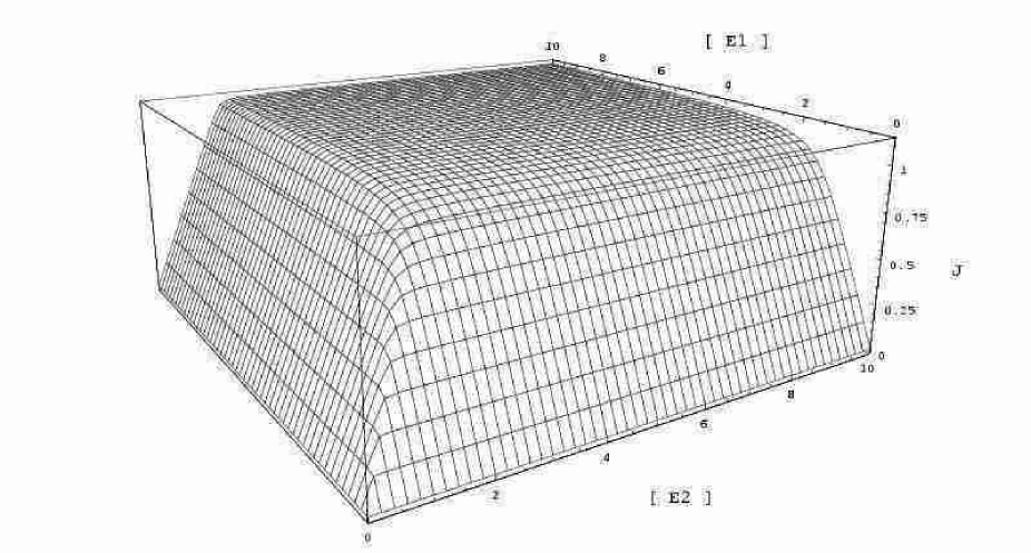
Figure 2: Metabolic flux as a function of total enzyme concentrations. The constant environmental input is $u=0.75$ mM. The catalytic turnover rates are symmetric such that $k_{cat(1)}=k_{cat(2)}=42,000min^{-1}$. Enzyme concentrations $[E_{i}]$ in $\mu M$. Flux in $mM~{}sec^{-1}$.

• 

• 

• 

• 

• 

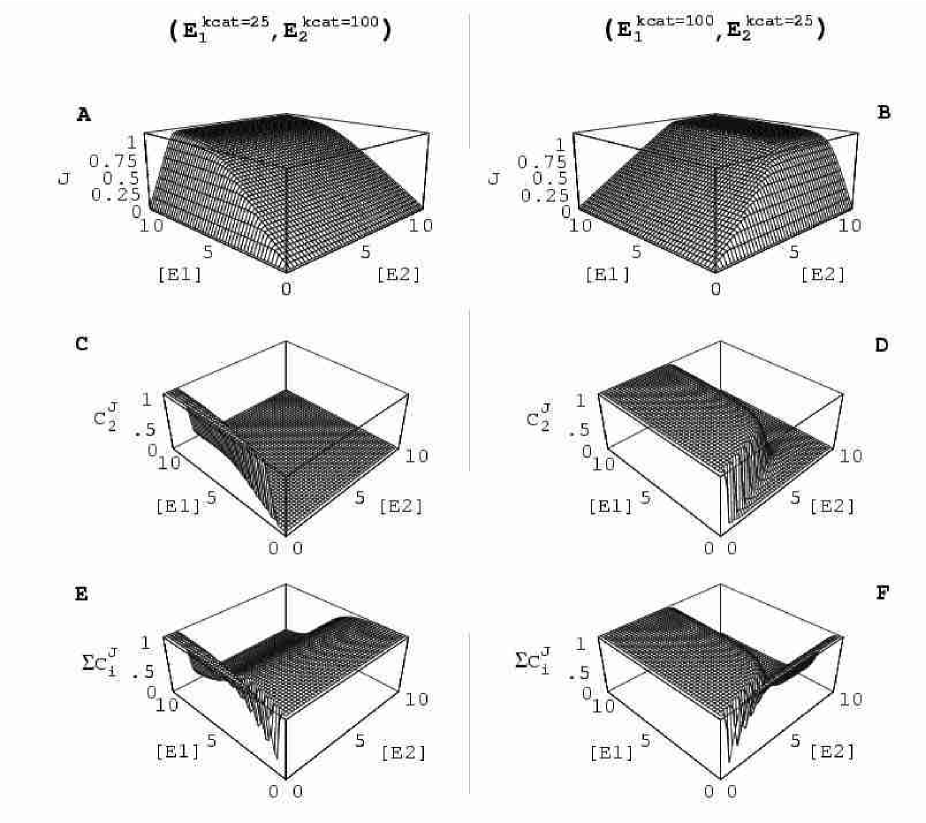
Figure 7: Changes in control of a pathway due to alteration of catalytic turnover rate $\bf k_{cat}$ ($k_{cat(i)}=100=42,000min^{-1}$). Enzyme concentrations $[E_{i}]$ in $\mu M$. For both enzymes $\delta E_{i}=0.02\mu M$.

• 

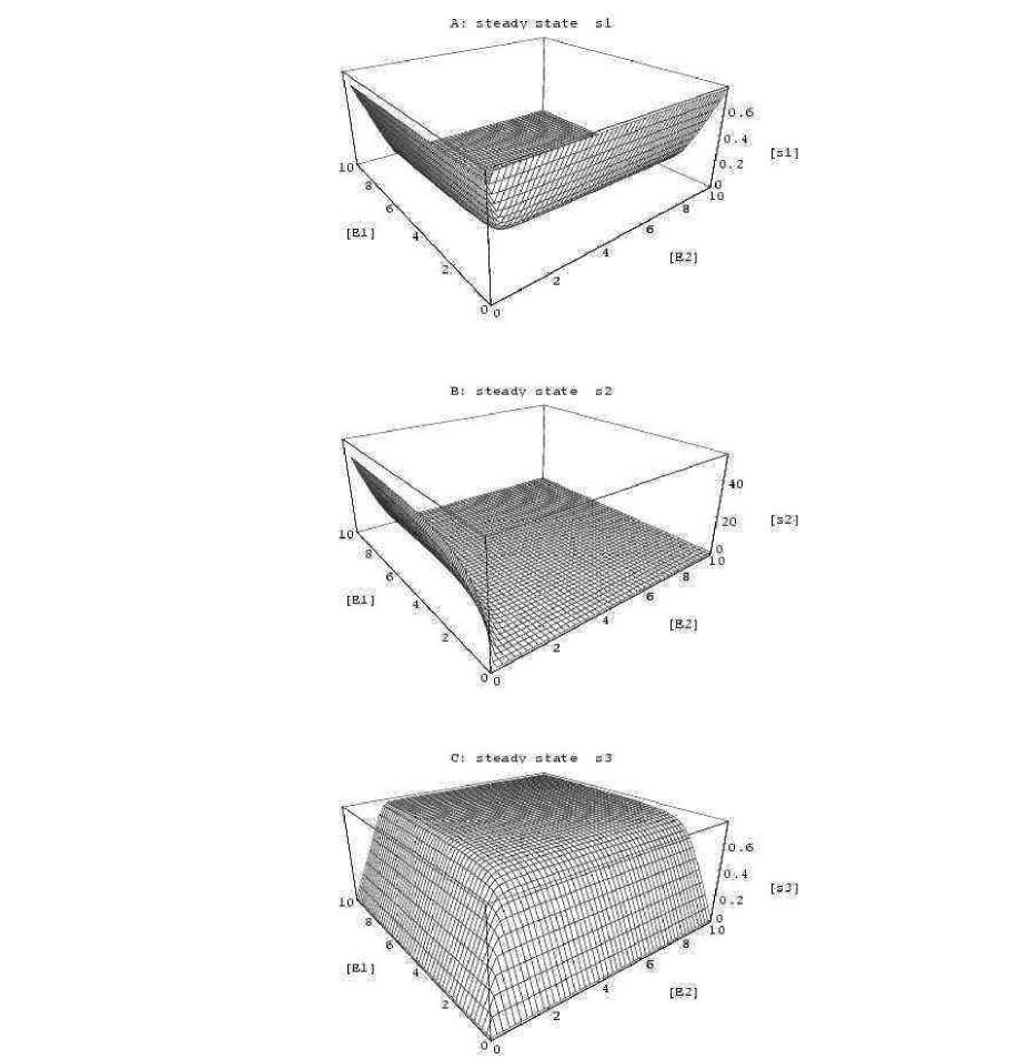
Figure 8: Steady state substrate concentrations as a function of total enzyme concentrations in pathway $\bf p_{\ref{odes}}$. Horizontal axes: $\mu M$ units. Vertical axes: $mM$ units. ( see Appendix C ).

• 

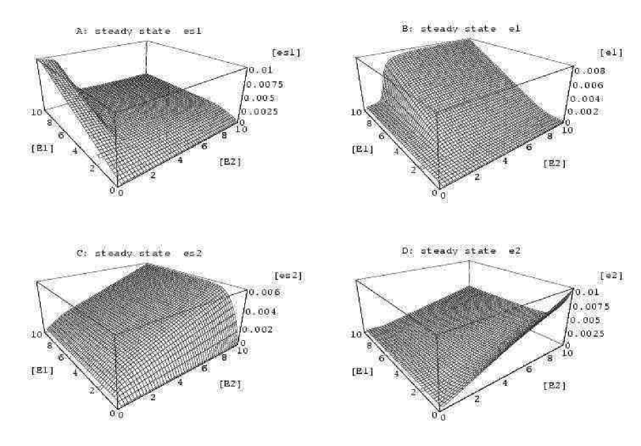
Figure 9: Steady state enzyme-substrate and free enzyme concentrations as a function of total enzyme concentrations in pathway $\bf p_{\ref{odes}}$. Horizontal axes: $\mu M$ units. Vertical axes: $mM$ units ( see Appendix C ).

• 

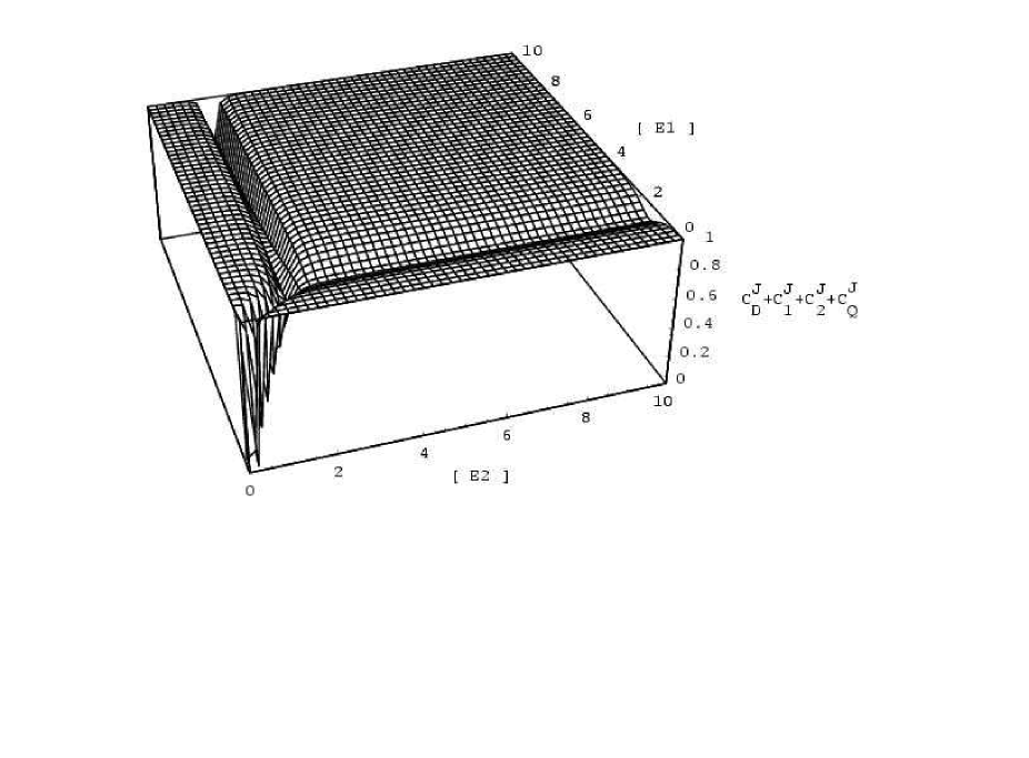
Figure 10: Failure of a modified summation conjecture.Enzyme concentrations $[E_{i}]$ in $\mu M$ (  see Appendix C ).

Bibliography

• Cornish-Bowden, 1987 Cornish-Bowden, A. (1987). Dominance is not inevitable. J. theor. Biol. 125, 333–338.
• Fontana & Buss, 1996 Fontana, W. & Buss, L. W. (1996). The barrier of objects: from dynamical systems to bounded organizations. In Boundaries and Barriers, (Casti, J. & Karlquist, A., eds), pp. 56–116. Addison-Wesley, Reading, MA.
• Giersch, 1988 Giersch, C. (1988). Control analysis of metabolic networks. Eur. J. Biochem. 174, 509–513.
• Grossniklaus et al., 1996 Grossniklaus, U., Madhusudhan, M. & Nanjundiah, V. (1996). Nonlinear enzyme kinetics can lead to high metabolic flux control coefficients: Implications for the evolution of dominance. J. theor. Biol. 182, 299–302.
• Heinrich & Rapoport, 1974 Heinrich, R. & Rapoport, T. A. (1974). A linear steady-state treatment of enzymatic chains. General properties, control and effector strength. Eur. J. Biochm. 42, 89–95.
• Kacser, 1987 Kacser, H. (1987). Dominance not inevitable but very likely. J. theor. Biol. 126, 505–506.
• Kacser, 1991 Kacser, H. (1991). A superior theory? J. theor. Biol. 149, 141–144.
• Kacser, 1995 Kacser, H. (1995). The control of flux: 21 years on. Recent developments in Metabolic Control Analysis. Bioch. Soc. Trans. 23, 387–391.
• Kacser & Burns, 1973 Kacser, H. & Burns, J. A. (1973). The control of flux. Symp. Soc. Exp. Biol. 27, 65–104.
• Kacser & Burns, 1979 Kacser, H. & Burns, J. A. (1979). Molecular democracy: who shares the controls? Bichem. Soc. Trans. 7, 1149–1160.
• Kacser & Burns, 1981 Kacser, H. & Burns, J. A. (1981). The molecular basis of dominance. Genetics, 97, 639–666.
• Kacser et al., 1995 Kacser, H., Burns, J. A. & Fell, D. (1995). The control of flux: 21 years on. The control of flux. Bioch. Soc. Trans. 23, 341–366.
• Keightley, 1996 Keightley, P. D. (1996). A metabolic basis for dominance and recessivity. Genetics, 143, 621–625.
• Kholodenko et al., 1998 Kholodenko, B., Rohwer, J., Cascante, M. & Westerhoff, H. (1998). Subtleties in control by metabolic channelling and enzyme organization. Mol. Cell. Biochem. 184, 311–320.
• Mayo & Burger, 1997 Mayo, O. & Burger, R. (1997). Evolution of dominance: a theory whose time has passed? Biol. Rev. 72, 97–110.
• Porteous, 1996 Porteous, J. W. (1996). Dominance-one hundred and fifteen years after mendel’s paper. J. theor. Biol. 182, 223–232.
• Savageau, 1976 Savageau, M. A. (1976). Biochemical Systems Analysis: A study of function and design in molecular biology. Addison-Wesley, Reading, MA.
• Savageau, 1992 Savageau, M. A. (1992). Dominance according to metabolic control analysis: major achievement or house of cards? J. theor. Biol. 154, 131–136.
• Savageau & Sorribas, 1989 Savageau, M. A. & Sorribas, A. (1989). Constraints among molecular and systemic properties: implications for physiological genetics. J. theor. Biol. 141, 93–115.
• Tralau et al., 2000 Tralau, C., Greller, G., Pajatsch, M., Boos, W. & Bohl, E. (2000). Mathematical treatment of transport data of bacterial transport systems to estimate limitation in diffusion through the outer membrane. J. theor. Biol. 207, 1–14.