The stochastic resonance mechanism in the Aerosol Index dynamics

Abstract

We consider Aerosol Index (AI) time-series extracted from TOMS archive for an area covering Italy $(7-18^{o}E;36-47^{o}N)$. The missing of convergence in estimating the embedding dimension of the system and the inability of the Independent Component Analysis (ICA) in separating the fluctuations from deterministic component of the signals are evidences of an intrinsic link between the periodic behavior of AI and its fluctuations. We prove that these time series are well described by a stochastic dynamical model. Moreover, the principal peak in the power spectrum of these signals can be explained whereby a stochastic resonance, linking variable external factors, such as Sun-Earth radiation budget and local insolation, and fluctuations on smaller spatial and temporal scale due to internal weather and antrophic components.

I Introduction

Over the last two decades, much attention has been devoted to study stochastic resonance (SR) as a model for many kinds of physical phenomena. The term ”stochastic resonance” describes a phenomenon whereby a weak signal can be amplified and optimized by the presence of noise. Stochastic resonance was introduced by Benzi et al. benzi ; benzi1983 and Nicolis nicolis in the field of the physics of atmosphere to explain the periodic recurrent ice ages. They used the two levels Budyko-Sellers potential Budyko for describing the incoming and outcoming radiation and added to it a weak periodic forcing, representing the small modulation of the Earth’s orbital eccentricity and a noise corresponding to variations on small time-scale respect to eccentricity. They found that the presence of the noise amplifies the periodic component, facilitating the jump of the system between the two levels synchronously with the periodical forcing. So they obtained ice ages as a peak, in the power spectrum of a temperature record, centered around the $100000$ year period and characterized by the correct amplitude. Since then, stochastic resonance has been observed in a large variety of physical systems, including bistable ring lasers, semiconductor devices, chemical reactions and neurophysiological systems gammaitoni . In the atmospheric field, only recently it appears another application of the SR. In fact, in 1994 El-Niño-Southern-Oscillation has been modeled with stochastic resonance with a periodic forcing of five years Tziperman ; Stone i.e. stochastic resonance is conjectured to have some relevance also at local climate scale. From these works, however, it seems to be a strong link between the fluctuations in the atmospheric medium (humidity, temperature, wind speed and direction, industrial emission and urban pollution) and the dynamics, that describes the atmospheric behavior on larger spatial and temporal scales. In this paper, we want to reconsider the relevance of SR on global climate scale but on smaller time scale, considering that periodic behaviours of Earth motion could induce stochastic resonance. In this study, we consider time-series representing distribution of tropospheric aerosols that surely are affected by Earth’s revolution and rotation motions. Actually much attention is devoted to a better understanding of the aerosol role in the radiation budget Andreae . The aerosol effect on climate is quantified in terms of radiative forcing, namely the net variation of radiation flux at the top of the atmosphere due only to radiative aerosol effects. A cooling effect of some aerosol (ash and sulfate aerosols) is well-documented Charlson1987 , while other types absorb solar radiation (dust, carbonic and silicaceous aerosols). At present, there are many activities addressed to study the optical properties of anthropogenic aerosols, for determining their influence on the radiative forcing Tegen1996 ; Charlson . The finding of SR into time series from troposheric aerosol should give some new insight on this topic.

II Datasets

We extracted time-series to analyze from the archive of TOMS (Total Ozone Mapping Spectrometer) Aerosol Index (AI hereafter). In particular we use the data retrieved from the measurements effected by Nimbus 7, an eliosynchronous satellite orbiting around the Earth from November 1978 to May 1993. The AI was determined using the backscattered radiances $(I_{340},I_{380})$ measured by TOMS at 340 and 380nm in the following way:

$$AI=-100\left[log\left(\frac{I_{340}}{I_{380}}\right)_{meas}-log\left(\frac{I_{340}}{I_{380}}\right)_{theor}\right]$$

where the subscripts meas and theor indicate respectively measured and theoretically computed quantities Torres1998 . This parameter gives an information on the aerosol optical depth and strongly depends on aerosol layer height and on the optical properties of the aerosols Hsu1999 . The AI is defined in such a way that it is positive for UV absorbing aerosols and negative for no absorbing ones, even if it assumes small negative values when absorbing aerosols are near the Earth’s surface, up to 1.5 km Hsu1999 . It is important to underline that the clouds are characterized by a null AI, but their influence on the measurements is not negligible. In fact the presence of clouds can act as a screen for the detection operations, at least in the case of clouds covering large areas Torres1998 . The data have a spatial resolution of $1^{o}$ latitude x $1.25^{o}$ longitude (corresponding to 50km x 50km) and temporal resolution of one sample a day. At this time, we consider only a restricted area relative to Italy with the following geographical coordinates $(7-18^{o}E;36-47^{o}N)$. To reduce the clouds contribution on our data, we used the reflectivity data from TOMS as parameter to distinguish the case of obscuring clouds from not one. If the reflectivity exceeds a threshold of $25\%$, we consider the AI as corrupted by clouds and we corrected this sample replacing the experimental value with the previous one plus a quantity chosen randomly among $0$, $0.1$ and $-0.1$, where $0.1$ is the instrumental error. The physical hypothesis underlying this correction is the small variability of the aerosol content in two days on a area of 50km x 50km. Moreover we have to take into account that the Nimbus 7 stability period started from the 1984, so we consider time-series extended from January 1984 up to May 1993 Herman .

III Analysis

The first step in examining AI data is to use standard linear and nonlinear analysis techniques to prove that we are in presence of a dynamics intrinsically stochastic. In fig. 1 we can see one scalar time-series and its power spectrum. The power spectrum shows two evident peaks: the principal peak corresponds to an annual period, while the second one is related to a period of about 6 days.

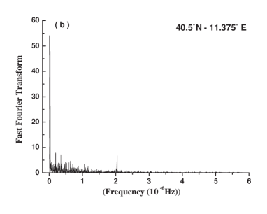
Figure 1: Example of Aerosol Index time-series (a) and its Power Spectrum (b) after the correction for reflectivity. Both the parts of the figure are related to an area of $1^{o}$ latitude x $1.25^{o}$ longitude centered at $40.5^{o}$ N - $11.375^{o}$ E.

For upgrading our knowledge about the dynamics generating these signals, as a first step, we apply the Independent Component Analysis (ICA) (Hyvarinen1999 and reference therein). It is a well established method, based on Information Theory, to extract, from a recorded signal, independent dynamical systems also non linear, but linearly superposed Acernese2000 . The ICA separates also noise.

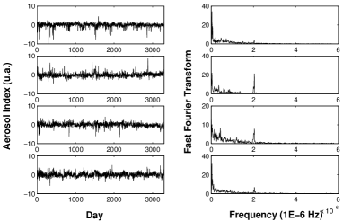
Figure 2: Result of the ICA application on 99 time-series recorded over Italy. We obtain 4 signals, but each of them still contains memory of the annual and weekly peaks as well as of the noise.

As we can observe looking at Fig.2, the application of ICA to our signals has not been able to separate noise contribution from deterministic one. So we may conclude that the periodic part of the signal is intrinsically tied to the fluctuations, i.e. our signals are generated by a genuine stochastic dynamics. Another confirmation of the stochastic nature of the dynamics can be derived from estimating embedding dimension. This estimate is made applying the False Nearest Neighbors method Kennel1992 to a single record: we obtain that up to dimension equal to 10 the algorithm does not converge as in the case of a stochastic process. In conclusion analyzing time series, it seems to be plausible to conjecture the presence of a mechanism of SR acting between the stochastic noise and the annual periodicity. It is important stressing that, if we conjecture SR as a global mechanism, it is also true that the parameters that rules the SR (local radiation budget and insolation) are characteristic of the site location. So it is clear that these parameters, as well as the noise level, depend on the width of the investigated area. In this first step, we focalize our attention on Italy $(7-18^{o}E;36-47^{o}N)$: we choose this particular area for investigating the contributes of both antrophic and natural aerosol sources and their mutual influence. Thus we have extracted 99 recorded series considering each one of them as a realization of the same stochastic process in a different spatial point. Since a comparison between two stochastic process can be made only on average, we have to extract the average series of experimental data that will be compare with that derived from the model. In this first analysis we devote our attention only to the dominant annual peak, so we execute a pass-band linear filter in the range of $10^{-9}-10^{-6}$ Hz. Successively, we eliminate from the signal a trend that can be ascribed to a residual trace of the satellite instability, obtaining the time-series represented in Fig.3. Now, finally, we have the experimental average time-series to be compared with the one derived from a simulated model.

IV Modelling

Figure 3: Experimental average signal relative to Italy $(7-18^{o}E;36-47^{o}N)$, filtered in the $10^{-9}-10^{-6}$ Hz range and subtracted of a residual trend [dotted line] and simulated one obtained averaging on 100 signals [solid line]. The parameters used in this simulation are $\textit{a}=0.3636$, $\textit{$A_{0}$}=437*10^{-4}$ and $\nu=0.06$

.

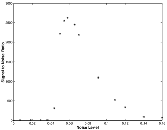
Figure 4: Estimate of the Signal to Noise Ratio obtained from the signal averaged over 100 realizations for each value of the noise level.

We have to mark two goals, the first is to numerically prove that our physical system can be effectively described with a resonance model, the second one is to make the best fit of the involved parameters and to give a physical interpretation of them. In the framework of the model used by Benzi et al. benzi ; benzi1983 , we described our physical system by means of the following equation:

$$dx=\left[\left(x-\frac{x^{3}}{a}\right)+Acos(\omega t)\right]dt+\nu$$

So we have considered a double well potential representing the radiative balance of incoming and outcoming radiation at the top of the atmosphere, that should be directly correlated with the different height of the aerosol layers in winter and summertime. This potential is completely characterized by the gap between them (gap that we indicate with a). The periodical component has a frequency of $3.2*10^{-}8$ Hz, corresponding to the annual peak, and amplitude $A$. This term is included to take into account the change of daily insolation with the solar declination angle. Because the short period disturbances can be described as a random walk hasselmann , the noise has been included as a Wiener process multiplied for a diffusion coefficient $\nu$. The estimate of parameters will give us the noise level, the amplitude of periodic forcing and then the estimate of difference between the two levels. Bearing in mind that, in regime of SR, the oscillation amplitude is equal to a, we fix this parameter in agree with the experimental average at the value of $0.3636$. So we have reduced the problem to determine the value of two parameters to better approximate our experimental signal.

Tuning the parameters we realize the time scale conditions gammaitoni finding the values that give us a maximum correlation integral between the mean value of the simulated stochastic process (obtained from 100 realizations for each value of the parameters) and the averaged experimental signal. In this way we find a maximum correlation integral of 0.71 corresponding to a dimensionless level noise of about 0.06 and an amplitude of periodic forcing equals to $437*10^{-4}$. The last quantity corresponds to the 10 percent of insolation variation over Italy, respect to the clear day solar insolation (estimated as $1000W/m^{2}$). With this simulation, we have the estimation of the parameters describing our system and we can also reconstruct the Signal to Noise Ratio (SNR) behavior as function of the noise strength. The SNR curve represented in Fig.4 is characteristic of the stochastic resonance gammaitoni : this confirms us that the AI dynamics can be described with a SR mechanism. Moreover the best approximating signal corresponds to a noise level of $\nu$=0.06, so in this curve of resonance we are around the maximum.

V Conclusions

The stochastic nature of the atmospheric medium is a well-established reality, but the enhancing function of this component is a no-trivial one. In this paper, we have proved that the Aerosol Index dynamics over Italy can be described through a stochastic resonance model and in addition we have found that we are effectively in stochastic resonance regime. This is an important aim, because it is the first time that SR is observed in atmospheric physics on human time scale. Surely this could be a fundamental tool for a better understanding of atmospheric dynamics, in particular for what concerns the links between the mechanism of global circulation and the local processes of aerosolic production and distribution. Moreover the presence of an atmospheric SR mechanism on a small time scale for the Aerosol Index has certainly some direct and indirect effects on other relevant atmospheric parameters such as the water vapor and precipitable water atmospheric contents, because of the aerosol’s role as condensation nuclei.

References

- (1) R.Benzi, A. Sutera, A. Vulpiani, J. Phy. A : Math. Gen. 1̱4,L453(1981).
- (2) R.Benzi, G. Parisi,A. Sutera, A. Vulpiani, SIAM J. Appl. Math. 4̱3, n.3, 565 (1983).
- (3) C. Nicolis, Tellus, 3̱4 , 1 (1982).
- (4) M.I. Budyko , Tellus ,2̱1, 611 (1969).
- (5) L. Gammaitoni, P. Hänggi, P. Jung, F. Marchesoni , Rev. Mod. Phys. ,7̱0, 1, 223 (1998).
- (6) E. Tziperman, L. Stone, M.A. Cane, H. Jarosh , Science, 2̱64, 72 (1994).
- (7) L. Stone, P.I. Saparin, A. Huppert, C. Price , Geophys. Res. Lett. 2̱5, 2, 175 (1998).
- (8) O. Andreae, J. Crutzen , Science , 2̱76, 1052 (1997).
- (9) R.J. Charlson, J. E. Lovelock, M. O. Andreae, S. G. Warren, Nature, 3̱26, 655 (1987).
- (10) I. Tegen, A.A. Lacis, I. Fung, Nature, 3̱80 , 419, (1996).
- (11) R.J. Charlson, S.E. Schwartz, J.M. Hales, R.D. Cess, J. Coakley, J.E. Hansen, D.J. Hofmann, Science, 2̱55, 423 (1992).
- (12) O. Torres, P.K.Bhartia , J.R.Herman, Z. Ahmad, J. Gleason, J. Geophys. Res. 1̱03,D14, 17099 (1998).
- (13) N.C. Hsu, J.R. Herman, O. Torres, B.N. Holben, D. Tanre, T.F. Eck, A. Smirnov, B. Chatenet, F. Lavenu, J. Geophys. Res. 1̱04,D6,6269 (1999).
- (14) J.R. Herman, P.K. Bhartia, O. Torres, C. Hsu, C. Seftor, E. Celarier , J. Geophys. Res. ,1̱02, D14, 16911 (1997).
- (15) A. Hyvärinen, E. Oja, Neural Computing Surveys, 2̱, 94 (1999).
- (16) F. Acernese, A. Ciaramella, S. De Martino, M. Falanga, R. Tagliaferri, Proceedings of the Second International Workshop on Independent Component Analysis and Blind Separation, Helsinki (2000).
- (17) M.B. Kennel, R. Brown, H.D.I. Abarbanel, Phys. Rev. A, 4̱5, 3403 (1992).
- (18) K. Hasselmann , Tellus ,2̱8, 473 (1976).