On reflection from a half-space with negative real permittivity and permeability: Time-domain and frequency-domain results
Jianwei Wang1 and Akhlesh Lakhtakia1
1CATMAS — Computational & Theoretical Materials Sciences Group
Department of Engineering Science and Mechanics
Pennsylvania State University
University Park, PA 16802–6812
ABSTRACT: The reflection of a normally incident wideband pulse by a half–space whose permittivity and permeability obey the one–resonance Lorentz model is calculated. The results are compared with those from frequency–domain reflection analysis. In the spectral regime wherein the real parts of the permittivity and the permeability are negative, as well as in small adjacent neighborhoods of that regime, the time–domain analysis validates the conclusion that it is sufficient to ensure that the imaginary part of the refractive index is positive — regardless of the sign of the real part of the refractive index.
Key words: negative real permeability; negative real permittivity; time–domain analysis
1 Introduction
Take a half–space occupied by an isotropic, homogeneous, dielectric medium of relative permittivity , where is the free–space wavelength. When a plane wave with electric field phasor of unit amplitude is incident normally on this half–space, the amplitude of the electric field phasor of the reflected plane wave is given by
| (1) |
where is the refractive index. The foregoing standard result is found in countless many textbooks; see, e.g., Born & Wolf [1] and Jackson [2]. It can be applied to insulators, poor conductors as well as good conductors.
Let the medium occupying the half–space also have magnetic properties represented by the relative permeability . Then, the previous result has to be modified as follows:
| (2) |
This result (2) for the reflection coefficient gains particular prominence in the context of composite materials that supposedly exhibit and in some spectral regime [3] — the time–dependence being implicit for all electromagnetic fields, with as the angular frequency. Shelby et al. [3] argued that the real part of must then be chosen to be negative. Consequently, it was concluded [5] that “[p]lane waves appear to propagate from plus and minus infinity towards the source …… [but] …… clearly energy propagates outwards from the source.” The conclusion has been employed to deduce the amplification of evanescent plane waves, leading to a proposal for aberration–free lenses [6].
Certainly, energy does not flow in the backward direction. Rather, the forward direction is defined as the direction of the energy transport, while the phase velocity may then be pointed in the backward direction — a known phenomenon [7]. Assuming the one–resonance Drude model for both and , confining themselves to the spectral regime wherein and , and impedance–matching the dielectric–magnetic half–space to free space, Ziolkowski and Heyman [4] pointed out that the reflection coefficient must have finite magnitude. Employing the one–resonance Lorentz model for both and , McCall et al. [8] recently deduced that
-
(i)
both and need not be negative for to be negative and to be positive, and
-
(ii)
the magnitude of the reflection coefficient does not then exceed unity.
Let us emphasize that the spectral regime for overspills into the neighborhoods of the regime wherein both and are negative.
Whereas frequency–domain analysis for the response of a half–space calls for the determination of the signs of and , the refractive index does not enter time–domain analysis. Therefore, time–domain analysis offers an independent way of assessing the results of frequency–domain analysis. In this communication, we present our conclusions from the response of a dielectric–magnetic half–space with negative real refractive index in a certain spectral regime to a normally incident wideband pulse. The Fourier transform of the reflected pulse confirms the frequency–domain calculations of in that spectral regime, and underscores the requirement of for real materials (which cannot be non–dissipative due to causality) to be sufficient.
2 Theory in Brief
Consider the region of spatiotemporal space. The half–space is occupied by a homogeneous dielectric–magnetic medium whose constitutive relations are given by
| (3) |
where the asterisk denotes the convolution operation [9] with respect to time, while the susceptibility functions
| (4) | |||||
obey the one–resonance Lorentz model. These susceptibility functions correspond to
| (5) | |||||
| (6) |
in the frequency domain [10]. In these expressions, and are the permittivity and the permeability of free space; is the speed of light in free space; is the unit step function; denote the so–called oscillator strengths; while and determine the resonance wavelengths and the linewidths. The region is vacuous.
At time , an amplitude–modulated wave is supposedly launched normally from the plane ; therefore, all fields are independent of and . The initial and boundary conditions on and are as follows:
| (7) |
Whereas is the carrier wavelength, the function
| (8) |
was chosen to represent the pulse. The cartesian unit vectors are denoted by .
The differential equations to be solved are as follows:
| (9) | |||
| (10) |
Their solution was carried out using a finite difference calculus described elsewhere in detail [11]. It suffices to state here that and were discretized into segments of size and , respectively; derivatives were replaced by central differences, and the leapfrog method was used [12].
Finally, the Fourier transform
| (11) |
was calculated to determine the spectral contents of the incident and the reflected pulses. The parameters , and were chosen to capture as much of both pulses as possible, following the procedure described elsewhere [11]. The computed ratio of the Fourier transform of the reflected pulse to that of the incident pulse is denoted here by , the subscript TD indicating its emergence from time–domain analysis.
3 Numerical Results and Discussion
For the sake of illustration, the following values were selected for the constitutive parameters of the dielectric–magnetic half–space: , , nm, nm, . Thus, and for all . However, is negative for nm, but it is positive for all other ; while is negative for nm, and positive for all other .
The definition of the refractive index in (2) suggests two possibilities: Either
-
A.
is negative for nm and positive elsewhere, consistent with the requirement of ; or
-
B.
is negative for nm and positive elsewhere, consistent with the requirement of .
Thus, our attention had to be focussed on the anomalous spectral regime nm. In this regime, the reflection coefficient for Possibility A is the reciprocal of that for Possibility B. The two possibilities can therefore be unambiguously distinguished from one another.
The carrier wavelength was chosen as nm. The pulse duration is fs and its 3dB band is nm. Therefore the anomalous spectral regime was substantively covered by our time–domain calculations. The segment sizes nm and fs used by us were adequate for the chosen constitutive parameters, but obviously would be totally inadequate in the resonance bands of and .
Possibility A is clearly nonsensical. It implies transport of energy in the half–space towards the interface . Not surprisingly therefore, (2), (5) and (6) yielded for all nm.
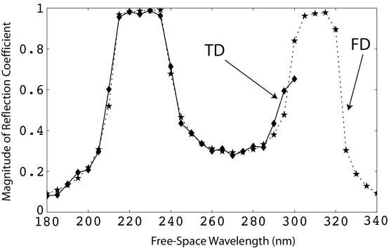
Figure 1 presents the computed values of obtained from (2), (5) and (6) for Possibility B (i.e., when is guaranteed for all ). The computed values of are also shown therein. The two sets of magnitudes compare very well for nm. Examination of the refracted pulse also showed that it transported energy away from the interface , which corroborates the observations of Ziolkowski and Heyman [4].
Thus, time–domain analysis validates the conclusion that must be selected in frequency–domain research in such a way that — irrespective of the sign of .
References
- [1] M. Born and E. Wolf, Principles of Optics, Pergamon, Oxford, UK, 1987, p. 41.
- [2] J.D. Jackson, Classical Electrodynamics, Wiley, New York, 1999; p. 306.
- [3] R.A. Shelby, D.R. Smith and S. Schultz, Experimental verification of a negative index of refraction, Science 292 (2001), 77–79.
- [4] R.W. Ziolkowski and E. Heyman, Wave propagation in media having negative permittivity and permeability. Phys Rev E 64 (2001), 056625.
- [5] D.R. Smith and N. Kroll, Negative refractive index in left–handed materials, Phys Rev Lett 85 (2000), 2933–2936. [These materials do not possess either structural or intrinsic chirality.]
- [6] J.B. Pendry, Negative refraction makes a perfect lens. Phys Rev Lett 85 (2001), 3966–3969. [See also correspondence on this paper: G.W. ’t Hooft, Phys Rev Lett 87 (2001) 249701; J. Pendry, Phys Rev Lett 87 (2001) 249702; J.M. Williams, Phys Rev Lett 87 (2001) 249703; J. Pendry, Phys Rev Lett 87 (2001) 249704. In addition, see appraisals by Ziolkowski & Heyman [4] and Lakhtakia (arXiv:physics/0112004 on http://xxx.lanl.gov).]
- [7] See the many instances cited by: I.V. Lindell, S.A. Tretyakov, K.I. Nikoskinen and S. Ilvonen, BW media — Media with negative parameters, capable of supporting backward waves, Microw. Opt Technol Lett 31 (2001), 129–133.
- [8] M.W. McCall, A. Lakhtakia and W.S. Weiglhofer, The negative index of refraction demystified. University of Glasgow, Department of Mathematics Preprint No. 2001/30.
- [9] J.W. Goodman, Introduction to Fourier optics, McGraw–Hill, New York, 1968, p. 19.
- [10] C.F. Bohren and D.R. Huffman, Absorption and scattering of light by small particles, Wiley, New York, 1983, Sec. 9.1.
- [11] J.B. Geddes III and A. Lakhtakia, Time–domain simulation of the circular Bragg phenomenon exhibited by axially excited chiral sculptured thin films, Eur Phys J Appl Phys 14 (2001), 97–105; erratum: 16 (2001), 247.
- [12] N. Gershenfield, The nature of mathematical modeling, Cambridge Univ. Press, Cambridge, UK, 1999, Sec. 7.1.