Nonlinear analysis of bivariate data with cross recurrence plots

Abstract

We use the extension of the method of recurrence plots to cross recurrence plots (CRP) which enables a nonlinear analysis of bivariate data. To quantify CRPs, we develop further three measures of complexity mainly basing on diagonal structures in CRPs. The CRP analysis of prototypical model systems with nonlinear interactions demonstrates that this technique enables to find these nonlinear interrelations from bivariate time series, whereas linear correlation tests do not. Applying the CRP analysis to climatological data, we find a complex relationship between rainfall and El Niño data.

,

1 Introduction

A major task in bi- or multivariate data analysis is to compare or to find interrelations in different time series. Often, these data are gained from natural systems, which show generally nonstationary and complex behaviour. Furthermore, these systems are often observed by very few measurements providing short data series. Linear approaches of time series analysis are often not sufficient to analyse this kind of data. In the last two decades a great variety of nonlinear techniques has been developed to analyse data of complex systems (cf. [1, 2]). Most popular are methods to estimate fractal dimensions, Lyapunov exponents or mutual information [2, 3, 4, 5]. However, most of these methods need long data series. The uncritical application of these methods especially to natural data often leads to pitfalls.

To overcome the difficulties with nonstationary and rather short data series, the method of recurrence plots (RP) has been introduced [6, 7, 8]. An additional quantitative analysis of recurrence plots has been developed to detect transitions (e. g. bifurcation points) in complex systems [9, 10, 11, 12]. An extension of the method of recurrence plots to cross recurrence plots enables to investigate the time dependent behaviour of two processes which are both recorded in a single time series [13, 14]. The basic idea of this approach is to compare the phase space trajectories of two processes in the same phase space. The aim of this work is to develop further new measures of complexity, which are based on cross recurrence plots and to evaluate the similarity of the considered systems. This nonlinear approach enables to identify epochs where there are linear and even nonlinear interrelations between both systems.

Firstly, we give an overview about recurrence plots and cross recurrence plots and, than, we develop further new measures of complexity. Lastly, we apply the method to two model systems and to natural data.

2 Recurrence Plot

The recurrence plot (RP) is a tool in order to visualize the dynamics of phase space trajectories and was firstly introduced by Eckmann et al. [7]. Following Takens’ embedding theorem [15], the dynamics can be appropriately presented by a reconstruction of the phase space trajectory $\vec{x}(t)$ from a time series $u_{k}$ (with a sampling time $\Delta t$) by using an embedding dimension $m$ and a time delay $\tau$

$$\vec{x}(t)=\vec{x}_{i}=\left(u_{i},u_{i+\tau},\dots,u_{i+(m-1)\,\tau}\right),\quad t=i\,\Delta t.$$ (1)

The choice of $m$ and $\tau$ are based on standard methods for detecting these parameters like method of false nearest neighbours (for $m$) and mutual information (for $\tau$), which ensures the entire covering of all free parameters and avoiding of autocorrelation effects [2].

The recurrence plot is defined as

$$\mathbf{R}_{i,\,j}=\Theta\left(\varepsilon_{i}-\|\vec{x}_{i}-\vec{x}_{j}\|\right),$$ (2)

where $\varepsilon_{i}$ is a predefined cut-off distance, $\|\cdot\|$ is the norm (e. g. the Euclidean norm) and $\Theta(x)$ is the Heaviside function. The values one and zero in this matrix can be simply visualized by the colours black and white. Depending on the kind of the application, $\varepsilon_{i}$ can be a fixed value or it can be changed for each $i$ in such a way that in the ball with the radius $\varepsilon_{i}$ a predefined amount of neighbours occurs. The latter will provide a constant density of recurrence points in each column of the RP. Such a RP exhibits characteristic large-scale and small-scale patterns which are caused by typical dynamical behavior [7, 12, 10], e. g. diagonals (similar local evolution of different parts of the trajectory) or horizontal and vertical black lines (state does not change for some time). A single recurrence point, however, contains no information about the state itself.

As a quantitative extension of the method of recurrence plots, the recurrence quantification analysis (RQA) was introduced by Zbilut and Webber [10, 11]. This technique defines several measures mostly based on diagonal oriented lines in the recurrence plot: recurrence rate, determinism, maximal length of diagonal structures, entropy and trend. The recurrence rate is the ratio of all recurrent states (recurrence points) to all possible states and is therefore the probability of the recurrence of a certain state. Stochastic behaviour causes very short diagonals, whereas deterministic behaviour causes longer diagonals. Therefore, the ratio of recurrence points forming diagonal structures to all recurrence points is called the determinism (although this measure does not really reflect the determinism of the system). Diagonal structures show the range in which a piece of the trajectory is rather close to another one at different time. The diagonal length is the time span they will be close to each other and their mean can be interpreted as the mean prediction time. The inverse of the maximal line length can be interpreted to be directly related with the maximal positive Lyapunov exponent [7, 9, 16]; in this interpretation it is assumed that the considered system is chaotic and has no stochastic influences. Since real (natural) systems are always affected by noise, we suggest that this measure has to be interpreted in a more statistical way, for instance as a prediction time. However, if we consider a chaotic system, the maximal positive Lyapunov exponent is much more reflected in the distribution of the line lengths. The entropy is defined as the Shannon entropy in the histogram of diagonal line lengths. Stationary systems will deliver rather homogeneous recurrence plots, whereas nonstationary systems cause changes in the distribution of recurrence points in the plot visible by brightened areas. For example, a simple drift in the data causes a paling of the recurrence plot away from the main diagonal to the edges. The parameter trend measures this effect by diagonal wise computation of the diagonal recurrence density and its linear relation to the time distance of these diagonals to the main diagonal.

3 Cross Recurrence Plot

Analogous to Zbilut et al. [13], we will use the recently expanded method of recurrence plots to the method of cross recurrence plots, which compares the dynamics represented in two time series. Herein, both time series are simultaneously embedded in the same phase space. The test for closeness of each point of the first trajectory $\vec{x}_{i}$ ($i=1\dots N$) with each point of the second trajectory $\vec{y}_{j}$ ($j=1\dots M$) results in a $N\times M$ array $\mathbf{CR}_{i,\,j}=\Theta(\varepsilon-\|\vec{x}_{i}-\vec{y}_{j}\|)$ called the cross recurrence plot (CRP). Visual inspection of CRPs already reveals valuable information about the relationship between both systems. Long diagonal structures show similar phase space behaviour of both time series. It is obvious, that if the difference of both systems vanishes, the main diagonal line will occur black. An additional time dilatation or compression of one of these similar trajectories causes a distortion of this diagonal line [14]. In the following, we suppose that both systems do not have differences in the time scale and have the same length $N$, hence, the CRP is a $N\times N$ array and an increasing similarity between both systems causes a raising of the recurrence point density along the main diagonal until a black straight main diagonal line occurs (cf. Fig. 3). Finally, the CRP compares the considered systems and allows us to benchmark their similarity.

4 Complexity measures based on cross recurrence plots

Next, we will define some modified RQA measures for quantifying the similarity between the phase space trajectories. Since we use the occurrence of the more or less discontinuous main diagonal as a measure for similarity, the modified RQA measures will be determined for each diagonal line parallel to the main diagonal, hence, as functions of the distance from the main diagonal. Therefore, it is also possible to assess the similarity in the dynamics depending on a certain delay.

We analyze the distributions of the diagonal line lengths $P_{t}(l)$ for each diagonal parallel to the main diagonal. The index $t\in[-T\ldots T]$ marks the number of the diagonal line, where $t=0$ marks the main diagonal, $t>0$ the diagonals above and $t<0$ the diagonals below the main diagonal, which represent positive and negative time delays, respectively.

The recurrence rate $RR$ is now defined as

$$RR(t)=\frac{1}{N-t}\sum_{l=1}^{N-t}l\,P_{t}(l)$$ (3)

and reveals the probability of occurrence of similar states in both systems with a given delay $t$. A high density of recurrence points in a diagonal results in a high value of $RR$. This is the case for systems whose trajectories often visit the same phase space regions.

Analogous to the RQA the determinism

$$DET(t)=\frac{\sum_{l=l_{min}}^{N-t}l\,P_{t}(l)}{\sum_{l=1}^{N-t}l\,P_{t}(l)}$$ (4)

is the proportion of recurrence points forming long diagonal structures of all recurrence points. Stochastic as well as heavily fluctuating data cause none or only short diagonals, whereas deterministic systems cause longer diagonals. If both deterministic systems have the same or similar phase space behaviour, i. e. parts of the phase space trajectories meet the same phase space regions during certain times, the amount of longer diagonals increases and the amount of smaller diagonals decreases.

The average diagonal line length

$$L(t)=\frac{\sum_{l=l_{min}}^{N-t}l\,P_{t}(l)}{\sum_{l=l_{min}}^{N-t}P_{t}(l)}$$ (5)

reports the duration of such a similarity in the dynamics. A high coincidence of both systems increases the length of these diagonals.

High values of $RR$ represent high probabilities of the occurrence of the same state in both systems, high values of $DET$ and $L$ represent a long time span of the occurrence of a similar dynamics in both systems. Whereas $DET$ and $L$ are sensitive to fastly and highly fluctuating data, $RR$ measures the probabilities of the occurrence of the same states in spite of these high fluctuations (noisy data). It is important to emphasize that these parameters are statistical measures and that their validity increases with the size of the CRP.

Compared to the other methods, this CRP technique has important advantages. Since all parameters are computed for various time delays, lags can be identified and causal links proposed. An additional analysis with opposite signed second time series allows us to distinguish positive and negative relations. To recognize the measures for both cases, we add the index $+$ to the measures for the positive linkage and the index $-$ for the negative linkage, e. g. $RR_{+}$ and $RR_{-}$. A further substantial advantage of our method is the capability to find also nonlinear similarities in short and nonstationary time series with high noise levels as they typically occur, e. g., in biology or earth sciences. However, the shortness and nonstationarity of data limits this method as well. One way to reduce problems that occur with nonstationary data is the alternative choice of the neighbourhood as a fixed amount of neighbours in the ball with a varying radius $\varepsilon$. A further major aspect is the reliability of the found results. Until a mature statistical test is developed, a first approach could be a surrogate test.

In the next section we apply these measures of complexity to prototypical model systems and to real data.

5 Examples illustrating the CRP

5.1 Noisy periodic data

First, we consider a classical example to check whether our technique is there compatible with linear statistical tools: two sine functions $f(x)$ and $g(x)$ with the same period ($2\,\pi$), whereby the second function $g(x)$ is shifted by $\pi/2$ and strongly corrupted by additive Gaussian white noise $\xi\in[-1,1]$; the signal to noise ratio is 0.5 (Fig. 1). Both time series have a length of 500 data points with a sampling rate of $2\pi/100$.

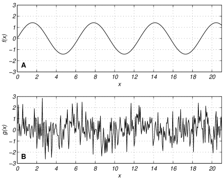
Figure 1: Two delayed sine functions, one of them corrupted by additive white noise (B).

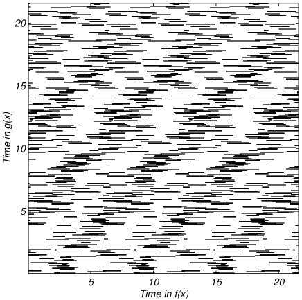
Figure 2: Cross recurrence plot for two delayed sine functions (Fig. 1) with an embedding of $m=3$, $\tau=\pi/2$ and $\varepsilon=1.5$. The diagonal lines in the CRP result from similar phase space behaviour of both functions.

We apply our analysis with $m=3$, $\tau=\pi/2$ and $\varepsilon=1.5$ (fixed radius, Euclidean distance). The CRP shows diagonal structures separated by gaps (Figs. 2). These gaps are the result of the high fluctuation of the noisy sine function. Due to the periodicity of these functions, the diagonals have a constant distance to each other equal to the value of the period $\lambda=2\,\pi$. The interrupted diagonal structures consist of a number of short diagonals. However, these are long enough to achieve significant maxima in the measures $RR$, $DET$ and $L$.

As expected, in this example the classical cross-correlation function shows a significant correlation after a lag of $\pi/2$ (Fig. 3A). The $RR$, $DET$ and $L$ functions also show maxima for positive and negative relation between $f(x)$ and $g(x)$. These maxima occur with the same lags $\pi/2$ like the linear correlation test (Fig. 3B-D). Despite the high noise level, these measures find the correlation. Hence, the result of this CRP analysis agrees with the linear correlation analysis.

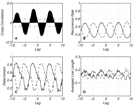
Figure 3: Cross-correlation (A), $RR$ (B), $DET$ (C) and $L$ (D) for two delayed sine functions. $L$ has the unit of time. The solid black lines show positive relation, the dashed lines show negative relation. The dash-dotted line in (A) marks the 5% confidence interval. All functions (A)–(D) detect the correlation after a lag of $\pi/2$.

Due to the noisy data, the trajectories strongly fluctuate in the phase space. Therefore, only short diagonal lines in the CRP occur and the means of the measures $DET$ and $L$ have (relative) small values.

5.2 System with nonlinear correlations

The next example is concerned to a nonlinear interrelation between systems. We will study this interrelation by using a standard linear method (cross correlation), a standard method from nonlinear data analysis (mutual information, cf. [2]) and the new proposed measures. We consider linear correlated noise (autoregressive process), which is nonlinearly coupled with the $x$-component of the Lorenz system $x(t)$ (solved with an ODE solver for the standard parameters $\sigma=10$, $r=28$, $b=8/3$ and a time resolution of $\Delta t=0.01$, [17, 18]). We use a first order autoregressive process $y_{n}$ and force it with the squared $x$-component

$$y_{n}=0.86\,y_{n-1}+0.500\,\xi_{n}+\kappa\,x_{n}^{2},$$ (6)

where $\xi$ is Gaussian white noise and $x_{n}$ ($x(t)\rightarrow x_{n}$, $t=n\Delta t$) is normalized to standard deviation $\sigma=1$ (Fig. 4). The data length is 8,000 points. The coupling $\kappa$ is realized without any lag. In order to study the behaviour of the proposed measures as a function of the coupling strength, we compute the CRPs for $\kappa\in[0,3]$ and for 500 independent realizations. The major periods of the system $x$ are 2.9 and 1.1, whereas the major periods of the selected realization of the system $y$ shown in Fig. 4 are 0.77, 0.96 and 0.59 (ordered from highest to lower).

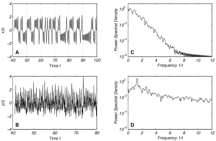
Figure 4: (B) Time series of a nonlinear related system consisting of a driven first order autoregressive process, forced by the squared (A) $x$-component of the Lorenz system ($\kappa=0.2$). The major periods (frequencies) are 2.9 (0.34) and 1.1 (0.94) for $x$ (C) and 0.77 (1.30) and 0.96 (1.05) for $y$ (D).

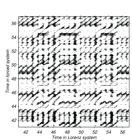
Figure 5: Cross recurrence plot for the forced autoregressive process $y$ (Fig. 4B) and the forcing function ($x$-component of the Lorenz system, Fig. 4A) for a coupling strength $\kappa=0.2$ and an embedding $m=5$, $\tau=10$, $\varepsilon=2$.

The cross correlation analysis of $x$ and $y$ do not reveal a significant linear correlation between them (Fig.6 A, B). The linear correlation does not increase for a growing coupling strength $\kappa$. However, the mutual information shows a strong dependence between $x$ and $y$ at delays of $0.05$, $-0.29$ and $0.44$ (Fig.6 C, D). This measure increases for a growing coupling. Analogous results can also be found with other nonlinear techniques which are designed for the study of interrelations as described in [19, 20].

The CRP of the driven AR-process (Eq. 6) with the $x$-component of the Lorenz system ($m=5$, $\tau=10$, $\varepsilon=2$) contains a lot of longer diagonal lines, which represent time ranges in which both systems have a similar phase space dynamics (Fig. 5). The results of the quantitative analysis of the CRP is strongly different from those of the linear analysis. It is important to note that the linear correlation analysis is here not able to detect any significant coupling or correlation between both systems (Fig. 6A and B).

Our measures of complexity exhibit the following: $RR$ and $L$ exhibit maxima at a lag of about $0.05$ for $RR_{+}$/ $L_{+}$ and $RR_{-}$/ $L_{-}$ and additionally at $0.45$ and $-0.32$ for $RR_{-}$/ $L_{-}$ (Figs. 7A, E). The delay of about $0.05$ stems from the auto correlation of $y$ and approximately corresponds to its correlation time $\Delta t/\ln{0.86}=0.066$. The other both delays are in the sum $0.77$ which suggests, that they are due to an interference of the main periods of the systems. $DET_{+}$ and $DET_{-}$ has also maxima at these delays, but these maxima are not significant in the sense that the values exceed the $2\sigma$-level of the $DET$ distribution gained from 500 realizations (Figs. 7C). This is due to the rapid fluctuating of $y$ and, thus, the less amount of longer diagonal structures ($l>3$). The reconstructed phase-space trajectories of $x$ and $y$ do not run parallel for some time.

The three measures have a slightly different dependence on the coupling strength $\kappa$: whereas $RR$ increases rather fast with growing $\kappa$, $DET$ increases slower and $L$ increases much slower with growing $\kappa$ (Figs. 7B, D, F). In comparison with the mutual information, the proposed measures have a similar regime, but especially $DET$ and $L$, spread stronger. However, this spread depends on the length of the considered data and decreases for longer data sets.

Finally we can infer, that the measures $RR$ and $L$ are suitable in order to find the nonlinear relation between the considered data series, where the linear analysis is not able to detect this relation. In this example, $DET$ does not reveal the nonlinear relation, because the rapidly fluctuation in $y$ kicks away the reconstructed phase-space trajectory from the parallel running to the trajectory of $x$. Since the result is rather independent of the sign of the second data before the embedding, the found relation is of the kind of an even function.

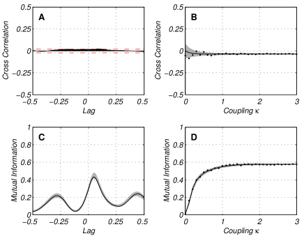
Figure 6: Cross-correlation (A, B) and mutual information (C, D) for the forced autoregressive process and the forcing function; A and C represents the measures for one realization as functions of the delay and for a coupling $\kappa=0.2$, B and D represents the measures for one realization (dots) and averaged (line) as functions of the coupling strength $\kappa$ (for a delay of zero). The dash-dotted lines in A mark the significance level of 5 % for the linear correlation between $x$ and $y$, the gray bands in B, C and D mark the $2\sigma$ margin of the distributions of the measures gained from the 500 realizations. The cross-correlation function does not find a significant correlation, but the mutual information shows significant interrelations between $x$ and $y$ at delays of $0.05$, $0.4$ and $-0.3$. The correlation coefficient does not clearly change for a growing coupling strength (B), however, the mutual information monotonically increases with a growing coupling strength $\kappa$ up to $\kappa=1$ and does not change for $\kappa>1$ (D).

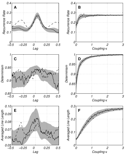
Figure 7: $RR$ (A, B), $DET$ (C, D) and $L$ (E, F) for the forced autoregressive process and the forcing function ($L$ has the unit of time). The solid lines show positive relation, the dashed lines show negative relation. The gray bands mark the $2\sigma$ margin of the distributions of the measures gained from the 500 realizations; only the $2\sigma$ margins for $RR_{+}$, $DET_{+}$ and $L_{+}$ are shown. $RR_{+}$/ $L_{+}$ and $RR_{-}$/ $L_{-}$ have clear maxima for a lag about $0.05$, $RR_{-}$ and $L_{-}$ have additionally maxima at $0.4$ and $-0.3$, which is the similar behaviour as the mutual information. The dependence from the coupling strength $\kappa$ is slightly different. Whereas $RR$ increases rather fast with growing $\kappa$ (B), $DET$ increases slower (D) and $L$ increases much slower (F) with growing $\kappa$. Since the maxima occur for $RR_{+}$, $DET_{+}$ and $L_{+}-$ as well as for $RR_{-}$, $DET_{-}$ and $L_{-}$, the found relation is of the kind of an even function.

5.3 Climatological data

The last example shows the potential of the CRPs in order to find interrelations in natural data. We investigate, whether there is a relation between the precipitation in an Argentinian city and the El Niño/ Southern Oscillation (ENSO). Power spectra analysis of local rainfall data found periodicities of 2.3 and 3.6 years within the ENSO frequency band [21].

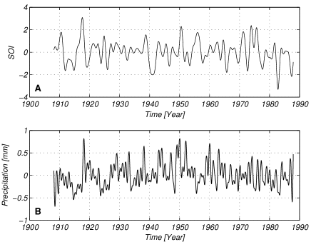
Figure 8: (A) Southern Oscillation Index (SOI) and (B) rainfall data of San Salvador de Jujuy.

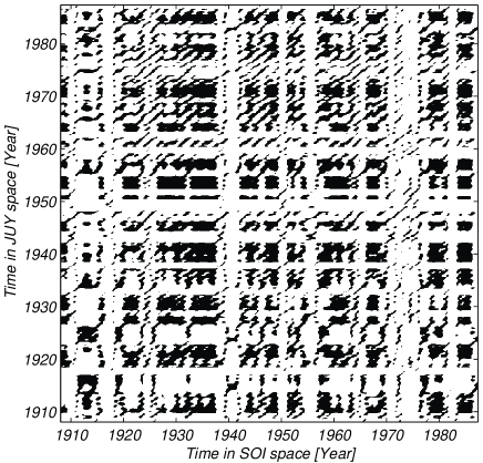
Figure 9: Cross recurrence plot of SOI vs. precipitation data from the city of San Salvador de Jujuy for an embedding of $m=3$, $\tau=4$ and $\varepsilon=1.3$). The $x$-axis shows the time along the phase space trajectory of the SOI and the $y$-axis that of JUY.

For our analysis we use monthly precipitation data from the city San Salvador de Jujuy in NW Argentina for the time span 1908–1987 (data from [22]). The behaviour of the ENSO phenomenon is well represented by the Southern Oscillation Index (SOI), which is a normalized air pressure difference between Tahiti and Darwin (Fig. 8; data from the Climate Server of NOAA, 1999, http://ferret.wrc.noaa.gov). Negative extrema in SOI data mark El Niño events and positive extrema La Niña events. We use the monthly SOI data for the same time span as the rainfall data. Both data sets have lengths of 960 points.

The cross correlation function and the mutual information show rather small correlation $\varrho=0.14$ between both data series with time delays of around 3 and 7 months, respectively (Fig. 10A, B).

After normalization of the data, the CRP with $m=3$, $\tau=4$ and $\varepsilon=1.3$ is calculated and shows several structures (Fig. 9).

The CRP analysis of local rainfall and SOI is done with a predefined shortest diagonal length $l_{min}=6$. The analysis reveals maxima for the complexity measures $RR_{+}$, $DET_{+}$ and $L_{+}$ for correlated behaviour around a delay of zero months, whereas the measures for anti-correlated behaviour $RR_{-}$, $DET_{-}$ and $L_{-}$ increase after about five months (Fig. 10). This result enables to conclude a positive relation between ENSO and the local rainfall. This gives some indication that the occurrence of an El Niño (extreme negative SOI) at the end of a year causes a decreased rainfall in the rainy season from November to January and the occurrence of a La Niña (extreme positive SOI) causes an increased rainfall during this time of the year. This conclusion extends the results obtained by power spectra analysis, where the similar periodicities in both SOI and local rainfall data were found [21]. These analysis show that a source for inter-annual precipitation variability in NW Argentina is the ENSO [21].

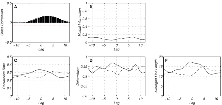
Figure 10: Cross correlation (A), mutual information (B) and CRP parameters (C, D, E) of SOI vs. precipitation data from the city of San Salvador de Jujuy (JUY). In C, D, E, the solid lines show positive relation, the dashed lines show negative relation. The dashed-dotted lines in (A) mark the 5% confidence interval. The maxima of the measures reveal an interrelation between the rainfall and the ENSO.

The linear correlation analysis finds the correlation, however, it is scarce above the significance and its mean at a lag of three months. The mutual information does not reveal a clear sign for interrelation between the data. It has small maxima at delays of $7$ and $-10$ months. In contrast, all the complexity measures $RR$, $DET$ and $L$ show a significant result and decomposite the correlation in a positive one with no delay and in a negative one with a delay of about five months, what suggests a more complex interrelation between the ENSO phenomenon and local rainfall in NW Argentina.

6 Conclusions

We have modified the method of cross recurrence plots (CRPs) in order to study the similarity of two different phase space trajectories. Local similar time evolution of the states becomes then visible by long diagonal lines. The distributions of recurrence points and diagonal lines along the main diagonal provides an evaluation of the similarity of the phase space trajectories of both systems. We have introduced three measures of complexity based on these distributions. They enable to quantify a possible similarity and interrelation between both dynamical systems. We have demonstrated the potentials of this approach for typical model systems and natural data. In the case of linear systems, the results with this nonlinear technique agree with the linear correlation test. However, in the case of nonlinear coupled systems, the linear correlation test does not find any correlation, whereas nonlinear techniques, as the mutual information, and the proposed complexity measures clearly reveal this relation. Additionally, the latters determine the kind of coupling as to be an even function. The application to climatological data enables to find a more complex relationship between the El Niño and local rainfall in NW Argentina than the linear correlation test, the mutual information or the power spectra analysis yielded.

Our quantification analysis of CRPs is able to find nonlinear relations between dynamical systems. It provides more information than a linear correlation analysis and the nonlinear technique of mutual information analysis. The future work is dedicated to the development of a significance test for RPs and the complexity measures which are based on RPs.

7 Acknowledgments

This work is part of the Special Research Programme Geomagnetic variations: Spatio-temporal structures, processes and impacts on the system Earth and the Collaborative Research Center Deformation Processes in the Andes supported by the German Research Foundation. We gratefully acknowledge M. H. Trauth and U. Schwarz for useful conversations and discussions and U. Bahr for support of this work. Further we would like to thank the NOAA-CIRES Climate Diagnostics Center for providing COADS data.

References

- [1] H. D. I. Abarbanel, R. Brown, J. J. Sidorowich, L. S. Tsimring, Rev. Mod. Phys. 65 (1993) 1331.
- [2] H. Kantz, T. Schreiber, Nonlinear Time Series Analysis, University Press, Cambridge, 1997.
- [3] J. Kurths, H. Herzel, An attractor in a solar time series, Physica D 25 (1987) 165–172.
- [4] B. B. Mandelbrot, The fractal geometry of nature, Freeman, San Francisco, 1982.
- [5] A. Wolf, J. B. Swift, H. L. Swinney, J. A. Vastano, Determining Lyapunov Exponents from a Time Series, Physica D 16 (1985) 285–317.
- [6] M. C. Casdagli, Recurrence plots revisited, Physica D 108 (1997) 12–44.
- [7] J.-P. Eckmann, S. O. Kamphorst, D. Ruelle, Recurrence Plots of Dynamical Systems, Europhysics Letters 5 (1987) 973–977.
- [8] M. Koebbe, G. Mayer-Kress, Use of Recurrence Plots in the Analysis of Time-Series Data, in: M. Casdagli, S. Eubank (Eds.), Proceedings of SFI Studies in the Science of Complexity. Nonlinear modeling and forecasting, Vol. XXI, Addison-Wesley, Redwood City, 1992, pp. 361–378.
- [9] L. L. Trulla, A. Giuliani, J. P. Zbilut, C. L. W. Jr., Recurrence quantification analysis of the logistic equation with transients, Physics Letters A 223 (1996) 255–260.
- [10] C. L. Webber Jr., J. P. Zbilut, Dynamical assessment of physiological systems and states using recurrence plot strategies, Journal of Applied Physiology 76 (1994) 965–973.
- [11] J. P. Zbilut, C. L. Webber Jr., Embeddings and delays as derived from quantification of recurrence plots, Physics Letters A 171 (1992) 199–203.
- [12] N. Marwan, N. Wessel, J. Kurths, Recurrence Plot Based Measures of Complexity and its Application to Heart Rate Variability Data, Physical Review E 66 (2) (2002) 026702.
- [13] J. P. Zbilut, A. Giuliani, C. L. Webber Jr., Detecting deterministic signals in exceptionally noisy environments using cross-recurrence quantification, Physics Letters A 246 (1998) 122–128.
- [14] N. Marwan, M. Thiel, N. R. Nowaczyk, Cross Recurrence Plot Based Synchronization of Time Series, Nonlinear Processes in Geophysics 9 (3/4) (2002) 325–331.
- [15] F. Takens, Detecting Strange Attractors in Turbulence, Vol. 898 of Lecture Notes in Mathematics, Springer, Berlin, 1981, pp. 366–381.
- [16] J. M. Choi, B. H. Bae, S. Y. Kim, Divergence in perpendicular recurrence plot; quantification of dynamical divergence from short chaotic time series, Physics Letters A 263 (4-6) (1999) 299–306.
- [17] E. N. Lorenz, Deterministic Nonperiodic Flow, Journal of the Atmospheric Sciences 20 (1963) 120–141.
- [18] J. H. Argyris, G. Faust, M. Haase, An Exploration of Chaos, North Holland, Amsterdam, 1994.
-
[19]
T. Schreiber, Measuring information transfer, Physical Review Letters 85 (2)
(2000) 461–464.
URL http://prola.aps.org/searchabstract/PRL/v85/i2/p461_1 -
[20]
A. Schmitz, Measuring statistical dependence and coupling of subsystems,
Physical Review E 62 (5) (2000) 7508–7511.
URL http://prola.aps.org/searchabstract/PRE/v62/i5/p7508_1 - [21] M. H. Trauth, R. A. Alonso, K. Haselton, R. Hermanns, M. R. Strecker, Climate change and mass movements in the northwest Argentine Andes, Earth and Planetary Science Letters 179 (2000) 243–256.
- [22] A. R. Bianchi, C. E. Yañez, Las precipitaciones en el noroeste Argentino, Instituto Nacional de Tecnologia Agropecuaria, Estacion Experimental Agropecuaria Salta, 1992.