Speed of light measurement using ping

Abstract

We report on a very simple and inexpensive method for determining the speed of an electrical wave in a transmission line. The method consists of analyzing the roundtrip time for ethernet packets between two computers. It involves minimal construction, straightforward mathematics and displays the usefulness of stochastic resonance in signal recovery. Using basic electrical properties of category-five cable students may use their measurements to determine the speed of light in the vacuum to within a few percent.

I. INTRODUCTION: With the now ubiquitous network and computer hardware in American secondary schools, high school and college students have become quite familiar with the internet. But the fact that signals on the internet cables typically move at hundreds of millions of meters per second (about 2/3 of the speed of light) is completely lost in the page download-and-rendering time that students experience. This laboratory experience grew out of a desire to leverage the now ubiquitous computer and network resources in schools for a simple, cheap, quality laboratory in which students measure one of the most consequential natural constants, the fantastic speed of light.

The measurement of the speed of light${}^{\cite[cite]{[\@@bibref{Number}{speeddefn}{}{}]}}$ has a history that students generally find interesting${}^{\cite[cite]{[\@@bibref{Number}{asimov}{}{}]}}$. There are the early speculations about light of the philosophers followed by the failed attempts of the giants of physics, Galileo and Newton. The first measurement of the speed of light was by Danish Astronomer Olaus Roemer in 1675 who used the moons of Jupiter as a clock. He determined the speed to be some 3/4 of its (now defined) speed, and a more accurate (about 5%) measurement had to wait half a century until British Astronomer James Bradley in 1728 determined it using the aberration of light from distant stars caused by the change in the orbital velocity of the Earth over the course of the seasons. The first non-astronomical measurement of light’s speed is due to French physicist Jean-Bernard-Léon Foucault in 1849 using the (now classic) quickly rotating mirror setup used later notably by American physicist Albert Michelson. Foucault’s measurement was within a percent of the modern (defined) value. This time period was one of intense scientific scrutiny of electricity and magnetism. In 1856 German physicists W. Weber and F. Kohlrausch used Leyden jars and a ballistic galvanometer to determine a ratio of electric and magnetic coupling strengths that has the dimensions of speed, and, intriguingly, found that speed to be near Foucault’s value for light. All of this development preceded J. C. Maxwell’s ${}^{\cite[cite]{[\@@bibref{Number}{maxwell}{}{}]}}$ theoretical synthesis of light as an electromagnetic wave in 1865. In our physics laboratory the determination of the speed of light is a classic experiment involving quickly rotating mirrors or, more popular nowadays, a pulsed source${}^{\cite[cite]{[\@@bibref{Number}{maryjames}{}{}]}}$ or a determination of the wavelength and frequency of microwaves.

All of the many methods of determining the speed of light in common use in our introductory physics laboratory and discussed in the literature (See for example Refs. [4] [5] [6]) have their experimental and pedagogic difficulties. In the experiment we chose and that we describe below our goals included

(1) Simple Equipment: The setup would require minimal effort and a minimal use of dedicated, specialized laboratory equipment.

(2) Simple Analysis: The structure and meaning of the laboratory and the analysis of the data should be straightforward.

(3) Flexible: The design should incorporate elements that may be interchanged and manipulated to allow students to be creative.

(4) Time: It should be possible to complete the data collection for a measurement in a single two hour period.

(5) Cost: The apparatus should be of minimal cost.

(6) Quality: The experiment must provide a determination of the speed of propagation (in air or in cable) with errors that are consistently not more than several percent.

We chose a time-of-flight approach because it is straightforward both in meaning and in analysis. For example, no reference is made to waves or the wave nature of light and thus this laboratory can logically be done early in the second semester sequence. The approach is simply to reflect small data packets between two computers that are connected with ethernet card/cables and record the round trip time. This has the great advantage of being easy to set up and inexpensive, a few tens of dollars for the the cost of a few “category-5” (hereafter referred to as “cat-5”) and RG-58/U coaxial cables of different lengths. Such echo time signatures (in engineer’s parlance ’Time Domain Reflectometry’ or TDR) are used in sophisticated and expensive commercial network analysis equipment and this laboratory represents a very simplified version of these tools. It opens classroom discussion to a world of interesting questions regarding the physical fabric of the internet.

The disadvantages of this method are (1) the additional abstraction of the theoretical connection between cable radio waves (invisible light) and free space waves and (2) the fact that the results are not immediately apparent from run to run but involve some (again straightforward) data analysis to see the effect of changing the cable length.

In addition to the advantages presented by our goals described above, other advantages of this method are (1) it will further familiarize students with ping as a useful IP protocol and (2) it makes use of existing equipment (the computers and cable resources) that is easy to bring together for this laboratory yet of use elsewhere after the laboratory. This may be of particular advantage for high school physics class budgets.

Finally, the experiment can be understood at several different levels of depth. At the most superficial level, this laboratory excersizes students’ knowledge of the relation $d=vt$ and scientific notation. But on a deeper level, this laboratory introduces students to the idea of noise-assisted sub-threshold signal detection, which, in the modern physics jargon is called stochastic resonance.

Here’s the problem; the cable range of ethernet without a repeater is about 250 feet (that is, at most a few microseconds roundtrip in cat-5 cable) and actually all the tests described here are done in much shorter cat-5 cable (more practical for typical reuse) and coaxial cable lengths so that it can be done cheaply. A typical classroom can hold several experiments of this type, the cables being shared between pairs of computers (and thus lab groups). Since ping only returns roundtrip times as measured in microseconds the actual signal (which is the additional delay in a cable path of longer length) is below the (reported) resolution of ping.

The solution is to use noise. Although noise usually hampers one’s ability to measure a signal, in this experiment, noise in the form of randomly distributed small delays (microseconds) associated with machine response actually makes the measurement of the signal (nanosecond-long cable transit delays) possible. Without the noise, the experiment we describe here would be impossible! This concept of noise-assisted sub-threshold signal detection (hereafter; stochastic resonance) is of great value because it plays a role in a great variety of systems. For a readable introduction and overview of stochastic resonance see Ref. [7] and Ref. [10] for a bibliography. For example, stochastic resonance has been used to analyze climate patterns${}^{\cite[cite]{[\@@bibref{Number}{climate}{}{}]}}$ and plays a role in fundamental neuro-physiology${}^{\cite[cite]{[\@@bibref{Number}{neuro}{}{}]}}$. Part of the hidden pedagogic agenda of this laboratory is to introduce the concept of stochastic resonance in a hands-on way. How well this laboratory can actually get students to ponder that depends on the approach of the instructor. Our experience with this laboratory indicates that time differences on the order of 50 nanoseconds (or about 5 % of the threshold) are reliably resolvable.

II: Hardware, Software and Experimental Design

Hardware: The hardware requirements of this experiment are basically two computers with ethernet NIC (Network Interface Cards) cards and various cable lengths. There is no need for any network switches or hubs. We have used laptops, some with built in ethernet NIC and others with PCMCIA NIC and both work fine. Although we have not tried this experiment on desktop machines we are confident that the data quality is largely independent of the hardware.

However, besides portability, laptops are useful because we did learn that the return times depended somewhat on the line voltage. We ran the experiment only when the laptops were fully warmed up, charged and yet still plugged into the wall to ameliorate dependence on line/power variability.

For cabling, we used standard cat-5 cables and RG-58/U coax of various length. Both of these types of cables are reasonably inexpensive and can be used elsewhere in the laboratory and classroom. Finally, the lengths of cable used in this experiment are actually rather short. The longest cable we used was 60m, though reasonably good results in cat-5 can be done with half that (see Figure 6). We have tried to repeat this experiment in cat-3 cable and were unable to get a reproducible signal presumably due to the noisy EMI environment (cat-3 is not as tightly twisted and subject to much more cross-talk and environmental electrical noise). For more technical information about cables and ethernet relevant to this experiment consult Appendix A.

A crossover cable allows one to create a direct connection between two machines, obviating the need (and expense) of a hub/switch for this experiment. Of course, such cables are also quite handy when moving files between two machines that are not on the same network.

Alternatively, one can also use a hub or a switch and just straight-through cables of different lengths. We have tested that the experiment can be profitably done through a hub; our hub seemed to introduce an additional 25 microseconds of delay in the roundtrip time, but any timing noise associated with it’s activity apparently was negligible at the timing threshold.

Terminated cat-5 cables are typically sold in the ’straight-through’ configuration, that is, they are not cross-cabled, having instead identically terminated ends. Thus, for the purposes of this experiment we made a single short (about 2.6 meter) cross-cabled cat-5 gender changer (male on one end, female on the other) cable that we used in series with commercial straight-through cat-5 cable of various lengths.

For the second part of the experiment we measured the speed of propagation in a RG-58/U (standard 50 $\Omega$ coaxial cable) by again using different cable lengths. As described above, the reason for doing this was that the conversion from the measured speed to the speed of light in vacuum was easy to do by measuring geometrical and simple electrical characteristics of the cable. In terms of hardware, we simply added BNC females at a break in a single pair (orange or green) of a short (.95m) straight-through ethernet cable. This cable’s RJ45 ends were then plugged into the crossover gender changer and the BNC females were mated with BNC males on the RG-58/U cables of various lengths. Additionally, we did find it necessary to impedance match the cat5 onto the coax; the coax has an impedance of $50\Omega$ and cat-5 cable of $100\Omega$. Figure 1 shows a schematic of the impedance matching circuit and a diagram of the shielded box used. Note that this arrangement allowed for only a rather short (about .05m) disturbance in the cat-5 cable.

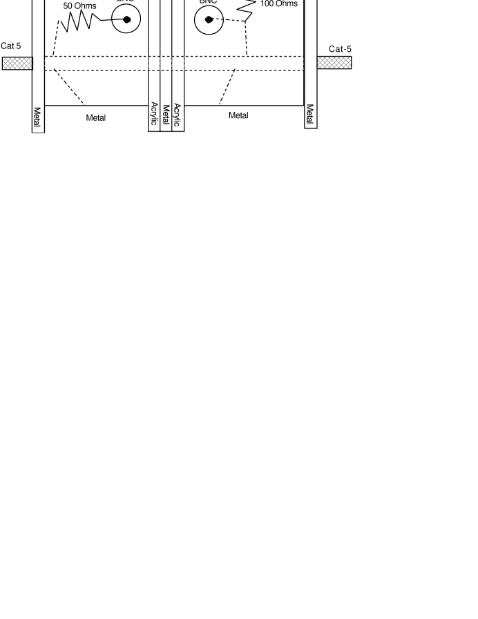
FIG. 1.: Cross Cable Impedance Matched onto RG-58/U Coax, and diagram of the shielded box

As such, the hardware requirements should be quite easy to meet for even the most restricted budgets. Again, when the experiment is finished or otherwise not in use the cables find use in connectivity in the rest of the lab/school.

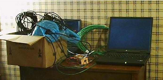
FIG. 2.: Picture of the Laboratory Setup during coax runs.

Software: We took data while running Linux on both computers. Although it should be possible to do this experiment with the new release of ping for Windows, because the authors were unfamiliar with Windows, Linux was chosen.

The Linux operating systems (OS) used (both Red Hat and Slackware) are free and widely distributed. These releases come with a system utility called ping which basically broadcasts a small (usually less than 100 bytes) IP packet through a specific internet adapter to another machine (specified by its IP address) on the network. That machine basically acts as a mirror. The packet header identifies the packet as a ping command and a process running on the ’mirror’ identifies it and rebroadcasts it (back) to the sender. The sender than checks the reflected packet for errors and reports the total roundtrip time. Ping has evolved much over the years; in the current Linux releases it reports the roundtrip time to the nearest microsecond whereas older versions only return the roundtrip time to the nearest millisecond. In this experiment we used the current version of ping.

Here is an example of the output of a basic ping command, in this case a computer ping-ing itself (the very first line (bold) was actually the command entered, the rest is output).

$>$ ping 168.192.0.10

PING 168.192.0.10 (168.192.0.10) from 168.192.0.10 : 56(84) bytes of data.

64 bytes from 168.192.0.10: icmp_seq=0 ttl=255 time=576 usec

64 bytes from 168.192.0.10: icmp_seq=1 ttl=255 time=82 usec

64 bytes from 168.192.0.10: icmp_seq=2 ttl=255 time=78 usec

64 bytes from 168.192.0.10: icmp_seq=3 ttl=255 time=78 usec

64 bytes from 168.192.0.10: icmp_seq=4 ttl=255 time=76 usec

— 168.192.0.10 ping statistics —

5 packets transmitted, 5 packets received, 0% packet loss

round-trip min/avg/max/mdev = 0.076/0.178/0.576/0.199 ms

Each of these five packets have been sent about one second apart. The transcript always includes a summary (at the end) indicating how many packets completed the reflection/reception successfully and, importantly, gives some gross statistics for the pings including the average round trip time to the nearest microsecond.

We found four switches, the -f the -i the -q and the -c, of ping quite useful for this experiment. The -f or ’flood’ switch instructs the ping daemon to keep sending out a new packet as soon as an earlier packet is received back. Because this can put some strain on a real network this command can only be executed by a user with root or ’superuser’ privilege, although for our two-computer network this is not a concern. The command ping -f $<$IPaddress$>$ is very useful in that it can quickly tell you whether there is enough fidelity on a particular cable to warrant running the experiment. If ping -f returns with many dropped (non-returned, or lost) packets OR if multiple applications of it reveal that there is not a steady (up to $\pm$ 1 microsecond) average return time, then the cable may not be suitable for this experiment or there are other sources of drift which will complicate the data collection/analysis of the experiment.

The command ping -i .01 $<$IPaddress$>$ issues a new packet every .01 seconds. This is used in the data collection since it it allows a student to accumulate on the order of one hundred thousand of pings in about 15 minutes. Large datasets are a necessity for subthreshold signal detection, and going to ten or 15 minute data collection times allows sufficient averaging of the noise so that signals (i.e. delays) on the order of 1/20^th of the threshold (i.e. about 50 nS) can be reproducibly resolved, yet in short enough time that the data acquisition can be completed in a lab period.

Ping reports time in microseconds, but it is not clear a priori how well its time measurement is calibrated. In order to calibrate the roundtrip times reported by ping we found the ping -q and ping -c commands quite useful. The switch -q simply forces ping to run quietly until the end when it writes its summary data to the ’standard I/O’ (the users screen). This means that while the system is running ping it has only the overhead associated with acknowledging the packet reception and issuing the next packet transmission. The rest of the time the system is waiting for the packet to return. Finally, the -c #N tells pings to run for exactly #N send-and-receive cycles.

It is easy to calibrate the ping times by combining the ping switches described above with the Linux time. The time command returns the system time, user time and overall time it takes for a command to complete. For example, for the particular experimental configuration that we used (whose full specification is below in the “Case Study” section) we issued the command (as root on the fast machine as described in the Experimental Design section below) “time ping -rfqc 300000 $<$IPaddress$>$” where $<$IPaddress$>$ was the IP number of the other machine. This runs the ’flood’-style ping for exactly 300000 times between the machines, returns summary data both from ping and from time. There is a noticeable (at the few percent level) difference between the reported ping times and the actual run time of the command, and in the case study below we use the difference to calibrate ping ’s microseconds.

Finally, in order to insure prompt packet handling, it is necessary to configure our machines so that they are on a common IP subnet. For example, if the machines are setup with a subnet mask of (the traditional) 255.255.255.0, then both machines must have the same first three numbers in their IP address, for example, 168.192.0.13 and 168.192.0.14.

Experimental Design: The basic idea of the experiment is to record round-trip ping times on two machines connected by a cable and to analyze how the average round-trip time changes when the cable’s length is changed.

In the actual experiment the computers and cables were not moved. Their batteries were fully charged and they were continuously plugged into wall power source for the entire duration of the data collection. After allowing them to warm up for about an hour while pinging ping -f and ping -i .01 to make sure the card and line were working properly, the mirror machine was reset so that there were no extraneous processes running on it (no users logged in or any batch activity other than what the basic system requires). Similarly, the transceiver machine was dropped into a text shell as root. This leads to a stable enough environment for the machines and their network that the data analysis is relatively straightforward (see below).

The data collection then commenced with a “ping -i .01 $<$IPaddress$>$  $>$ tempfile1.txt” where “$>$” (the so called ’pipe’ symbol) in unix/Linux means that the output is redirected to the disk file “tempfile1.txt”. This was allowed to run for 11 minutes or so and then stopped, another cable length inserted and the command rerun, now with the data piped to a (differently) named file (i.e. “tempfile2.txt”), and so on, until a series of runs were completed with various cable lengths. Ten runs with three or four different cable lengths can quite easily be completed in a two-hour laboratory period. In principle, staggering the order of cable lengths tested allows one some control of any systematic drift in the equipment over time. In practice that allowed us to verify that drift over the course of two hours was smaller than the resolution ( 50 nS) and so could be ignored, further simplifying the data analysis.

Each raw data file (’tempfile.txt’ in the description above) is a few megabytes. It is processed so that it ultimately consists of just two columns, the attempt number and the measured round-trip time for that ping attempt. Simple cuts are made (see details in the case study below) and the average and standard deviation of the remaining roundtrip times is computed and recorded. This analysis is straightforward enough to be done in a spreadsheet. Finally, the roundtrip distance (or cable length for the case of the coaxial cable) is plotted against average roundtrip time and (least-squares) fit with a line, the slope of which is the measured speed of signal propagation.

A more subtle point has to do with the properties that the timing noise must possess in order for it to faithfully assist the subthreshold signal detection. The relevant ping return times typically form a cluster about a few microseconds wide on a typical return time of hundreds of microseconds (see Figure 4). Thus, as long as the distribution of timing noise is relatively flat near the hundred microsecond band, the noise will faithfully assist in subthreshold signal detection. That this is indeed the case is evidenced by the reproducibility and data quality of the runs, allowing the reproducible average round-trip time resolution of about 50 nS (or 1/20th of ping’s reported resolution).

III. Case Study Example and Data Analysis Summary

Figure 2 shows a typical graph of round-trip times for the setup described above (in this case we use a 3.53m cat-5 crossover cable between a Gateway Solo 9500 (950 MHz with 100BT ethernet built in) running Red Hat Linux 7.1 and a Gateway Solo 2300 (with a 10BT 3COM589 PCMCIA slot ethernet card) running Slackware Linux 2.0.35). As such, note that the cable actually is running at 10BT speeds. We did however find similar data and data quality on other combinations of machines and speculate that the particular hardware doesn’t matter, as long as the machines are not identical (which might complicate the stochastic resonance).

FIG. 3.: Graph of 12,000 round-trip times as a function of attempt number, and detail

Note that most of these times cluster around 360 microseconds with a substantial set of outlyers, with some packets taking several milliseconds to return. The detail of the region around 360 microseconds indicates a spread in the main part of the data and characteristic timescales associated with longer recorded times. Additionally, there are periodic structures seen in these data; both the longer recorded times and the periodic structures we regard as extraneous; being the result of periodic and aperiodic disturbances associated with scheduled low-level tasks that are running in the OS. A histogram of the round-trip times of Figure 2 is shown below (Figure 3).

FIG. 4.: Same 12,000 roundtrip times in a log(frequency) histogram

These datafiles are then stripped of outlyers. We make a cut, for the example given above, keeping only those ping round-trip times of 365 microseconds or less and analyse all of the data sets in these runs with this same cut. (We found that the choice of the cut did not substantially affect our measured propagation speeds, the sensitivity to reasonable but different choices of cuts being at about the 0.5 percent level. Also, although we did not have a lower cut on the data, each million or so pings we occasional found a return time logged as 0 microseconds. These very rare spurious lines were also removed from the datasets. We used Interactive Data Language (IDL^tm) for the data analysis, fitting and plotting. The data analysis steps are elementary and may also be easily automated for an introductory class setting, or could be done on a spreadsheet or easily in Maple^tm or Matlab^tm. For the data set above we find that the data so filtered has a reported average round-trip time of 360.12 microseconds and a standard deviation that is about .64 microseconds, an error figure much bigger than the resolution we are claiming. It is due primarily to the width of the bins that the data is in, and is not a good measure of how well one can find the center of (an assumed nearly) gaussian distribution from these coarse data.

To calibrate the time reported by ping we issue a time ping -rfqc 300000 $<$IPaddress$>$ from the prompt and find an average roundtrip reported packet time of 369 $\mu$S and so the reported time spent waiting for the packets to return is 300000 $x$ 369 x 10${}^{-}6$ = 110.7 seconds. The time command returns a total time of 111.3 seconds, of which 4.02 seconds are spent in system calls for both the maintenance of the OS (which wasn’t doing any extraneous jobs) and the low-level ping system calls. This means basically 107.3 seconds were spent waiting for the ping s to return. Thus, the actual reported ping times were longer than the actual times by about 3%. We include this systematic error in our determination of the speed of propagation in the data analysis that follows.

Having done the same cut and tally with datsets for all five cable lengths (adding a length of .75, 3.07, 15.03, 37.5 and 57.15 meters to the gender change cross cable) we plot twice the category-5 cable length versus the average round-trip times in Figure 5

FIG. 5.: Round Trip distance (meters) versus round trip time (microseconds) in Cat-5 cable.

The least squares fit to these data yields a slope of 2.04$\pm$.14 x 10${}^{8}~{}{{m}\over{s}}$, indicating that the speed of propagation in a cat-5 cable is some 2/3 the speed of light in the vacuum.

Finally, in order to use this technique to estimate the speed of light in the vacuum we need some way of converting our cable measurements. This can easily be done with elementary electromagnetics theory for simple cable geometries. As a first approximation, the twisted pair in category 5 cable can be modeled as an (untwisted) pair of parallel wires each of radius $r$ completely surrounded by a dielectric material (the insulation, dielectric constant $\epsilon$) and with their centers held a distance $d$ apart. The capacitance per unit length of this system can be found by a straightforward application of the method of images, and the inductance can be found by integrating the magnetic flux between two current-carrying wires. The capacitance and inductance per unit length for such a transmission line is thus a standard computation yielding,

$$c={{\pi\epsilon\epsilon_{0}}\over{\log\bigl{(}{{d}\over{2r}}+\sqrt{{{d^{2}}\over{4r^{2}}}-1}\bigr{)}}}\qquad\qquad l={{\mu_{0}}\over{\pi}}\log\bigl{(}{{d-r}\over{r}}\bigr{)}+{{\mu_{0}}\over{4\pi}}\rho(\omega)$$ (1)

with $\rho(0)=1$ and $\rho(\infty)=0$ is a function associated with the skin effect in the conductor. At the frequencies of interest here $\rho\sim 1$. The telegrapher’s equation indicate that the speed of propagation ($v=1/\sqrt{cl}$) for electromagnetic waves along the transmission line and line impedance ($z=\sqrt{{{l}\over{c}}}$) for this cable are,

$$v=c_{0}\sqrt{{{\log\bigl{(}{{d}\over{2r}}+\sqrt{{{d^{2}}\over{4r^{2}}}-1}\bigr{)}}\over{\epsilon~{}\log\bigl{(}{{d-r}\over{r}}e^{1/4}\bigr{)}}}}\qquad\qquad z={{z_{0}}\over{\pi}}\sqrt{{{1}\over{\epsilon}}\log\bigl{(}{{d}\over{2r}}+\sqrt{{{d^{2}}\over{4r^{2}}}-1}\bigr{)}~{}\log\bigl{(}{{d-r}\over{r}}e^{.25}\bigr{)}}$$ (2)

Where $c_{0}$ and $z_{0}=377~{}\Omega$ are the speed of light in the vacuum and the impedance (in Ohms) of free space respectively. These expressions can be compared to other, more approximate expressions in the literature such as $c=0.276~{}{\rm x}~{}10^{-10}\epsilon/\log(d/r)$, $l=0.400~{}{\rm x}~{}10^{-6}\log(d/r)$ and $z=120.\log(d/r)/\sqrt{\epsilon}$ from Ref.[13].

For cat-5 cable, $r$ = .00026m and $d$ = .00086m. The DC capacitance per unit length of a pair in cat-5 cable is measured (by a DVM) to be about 45pF/meter, so this indicates that the dielectric constant at low frequency is $\epsilon=1.76$ where we have used Eq. (1). Thus the line impedance is computed by Eq. (2) to be $z=98\Omega$, in rough agreement with the specifications for cat-5. Assuming this is the same dielectric constant at radio (ethernet) frequencies, we use Eq. (2) and our data thus imply a speed of light in vacuum of $c_{0}=2.70\pm.18~{}{\rm x}~{}10^{8}{{m}\over{s}}$.

The main error in this determination of the speed of light in a vacuum using cat-5 cable data seems to be systematic effects associated with deficiencies in our model. We now estimate these effects. The twisting reduces the line impedance (chiefly by increasing the capacitance per unit length through the ’extra’ metal that the full twists effectively act as metal loops around the other conductor) and increases the actual length of the line as compared with the above model of straight parallel wires. A twist length of .7 cm in these cables (see Appendix A) indicates that to straighten out the wires in a pair we must twist the wires around each other 140 times each meter. Secondly, the conductors are not submerged in dielectric, but the dielectric is actually quite thin and so use of Eq. (1) is suspect. The net effect of these model deficiencies is to reduce the speed of signal transmission as compared with two parallel conductors. Even between two pairs (with different twist length) in the same cat-5 cable there can be as much as a 10 % effect due to the twist length of the pair, with more twists per unit length associated with a smaller overall speed.

We can very approximately account for the systematic effect due to extra length caused by twisting of the lines. This is easy for students to correct for, either by actually comparing the lengths of a pair before and after straightening out or geometrically from the measured data above; the actual length $L$ of conductor inside a twisted pair of length $L_{0}$ is simply $L=L_{0}\sqrt{1+\bigl{(}{{\pi d}\over{l_{tw}}}\bigr{)}^{2}}$ where $d$ is as before and $l_{tw}$ is the twist length of the pair. For a typical cat-5 cable the computed actual length $L$ of the pair is some (for .7cm twist length) 7.2 percent longer than the cable length. Amending our untwisted estimate above by this ’geometrical’ correction, our measurement indicates that $c_{0}=2.90\pm.19~{}{\rm x}~{}10^{8}{{m}\over{s}}$, a 7 percent sigma, and well within one sigma from the defined value for the speed of light in the vacuum.

Although this is a reasonable outcome, in an attempt to simplify this laboratory by avoiding some of these dicey geometrical and electrical intricacies of cat-5 cables, we repeated the above laboratory in a geometrically simpler cable, RG-58/U, otherwise known as standard 50 $\Omega$ coaxial cable. We already described in the hardware section efforts we made to impedance match and shield the cable junctions. The radius of the inner conductor of RG-58/U is measured to be $r$= .00083m and the inner radius of the sheath is $R$=.00296m. For a interconductor dielectric $\epsilon$ we can again resort to elementary electromagnetics theory to ascertain that the capacitance and inductance per unit length of a coaxial cable is

$$c={{2\pi\epsilon\epsilon_{0}}\over{\log(R/r)}}\qquad\qquad l={{\mu_{0}}\over{2\pi}}\log(R/r)+{{\mu_{0}}\over{4\pi}}\rho(\omega)$$ (3)

(compare with Ref.[12]) Which again may be compared again with the perhaps more approximate results $c=0.555~{}{\rm x}~{}10^{-10}\epsilon/\log(R/r)$ and $l=0.200~{}{\rm x}~{}10^{-6}\log(R/r)$ from Ref.[13]. These analytical expressions lead to a speed of propagation and a line impedance of

$$v=c_{0}/\sqrt{\epsilon}+\ldots\qquad\quad z={{z_{0}}\over{2\pi\sqrt{\epsilon}}}\log(R/r)$$ (4)

where $c_{0}$ here is the speed of light in a vacuum. The $\ldots$ is associated with the second term in Eq. (3) for $l$. The measured DC capacitance per unit length of our cable to is 97 pF/m (see also Ref.[14], pg. 256). Eq. (3) thus indicates that the DC dielectric constant is 2.22, and, as a check, these data imply that the line impedance is $52\Omega$.

Four coax lengths, .333m, 11.61m, 25.0m, and 74.5m were used. The cuts were performed, averages taken and Figure 5 is a graph of the coax cable length (since only one of the twisted pairs lines is of variable length) versus average packet round-trip time.

FIG. 6.: Coaxial cable length (meters) versus trip time (microseconds).

Thus the measure speed of propagation of an electromagnetic wave in RG-58 coax is 1.27 +/- .09 x $10^{8}~{}{{m}\over{s}}$, over seven meters per nanosecond. This is substantially different than the $.57c_{0}$ expected by the above formulas.

It may be that reflections and attenuation in the line play an important role in understanding this discrepancy. Although we shielded and attempted to impedance match the cables, there may still have been enough reflections at the connectors to cause phase shifts that may have delayed the signal acquisition by the ethernet cards. Also, the matching circuit that we used causes about 75% of the signal power to be lost at the junction box. The reduced signal also suffers further diminution in transit. If an attenuated signal takes longer for the ethernet cards to detect this will be a systematic effect that would reduce the measured propagation velocity. Such an effect may not have been seen in the cat-5 sections because the ones we used were so short that at 10BT speeds there should have been less than 10dB of loss in even the longest cable.

IV. Conclusion and Critique

Using ping to measure the speed of propagation of electrical signals in a cable and thus to determine the speed of light works reasonably well (at the 7% level) in cat-5 cable.

For simplicity of execution and analysis, low cost, dual use and accuracy this laboratory is hard to top! Since this lab does not make use of any of the wave properties of light it will be simpler for students to do earlier in their second semester of physics. It does make use of basic internet-style resources that students may find useful later, and may stimulate students to think more about the usefulness of stochastic resonance phenomena.

Of course, the disadvantage of this method is that the student has to marshal some theory both conceptually (that electrical signals in a wire are like light) and analytically to relate their measurements to the measurement of the speed of light in the vacuum.

Our development of this laboratory indicates points for further study. We have not yet been able to definitively determine why the method works so poorly in coax, though we have some indications that the junction box we used may be part of the problem. An interesting observation in that regard is that we actually tested ganging coax cable lengths with the use of a barrel connector and found that the presence of the barrel significantly distorted the measured return times. Apparently barrels are not so well matched onto 50 Ohm coax. In any case, if one wants to build the lab based on the geometrically simpler RG-58/U cable, it is possible to buy network cards that are made for this cable and come with BNC female connectors installed.

Also, this all raises the obvious question as to why we didn’t redo the experiment with a wireless network card and hub. These can be bought at a modest cost and we did try to do this laboratory with wireless ethernet. However, due to peculiarities with small packet handling in the wireless protocol we used (IEEE 802.11b) the return times were far too long and noisy for stochastic resonance to work. We have not yet looked into doing this with IR links (which may be too short) or fiber links, but that is also a logical next step.

Acknowledgments We are thankful to Mark Welton and Ray Hoff for discussions on ethernet and cabling and to Jeff Carroll and the XEL team at Y.S.U.’s Center for Photon Induced Processes for the RG-58/U cable lengths used in the experiment.

This work was supported in part by a grant from the DOE EPSCoR grant DE-FG01-00ER45832, Research Corporation Cottrell Science Award #CC5285, a Cluster Ohio Grant from the Ohio Supercomputer Center, NASA grant NAG9-1166 and a Research Professorship 2001-2002 award from YSU. This work was (partially) supported by the National Science Foundation through a grant for the Institute for Theoretical Atomic and Molecular Physics at Harvard University and the Smithsonian Astrophysical Observatory.

Bibliography

Appendix A: More about Network Cables

Invariably a laboratory like this opens the classroom up to all sorts of discussions about what is ’really going on’ and about particulars of the physics of wave propagation in the physical fabric of the internet. In this appendix we have collected information about cables and computer networks that an instructor may find useful to consult for answers to some of the questions that students may ask as a result of doing this laboratory.

In the first part of the experiment cat-5 cable was used. It consists of 8 lines in 4 unshielded twisted pairs (UTP) and is terminated by a male RJ45 connector, which looks like a wide phone jack. The only pairs of direct relevance for our experiment are the green (green and white-green lines) and orange (orange and white-orange lines) pair. One of the pair (pins 1 and 2) is for transmission and one is for reception (pins 3 and 6). For the purposes of this experiment, all the cables could have been of cross-cable type, that is, the green pair and the orange pair are interchanged between the two RJ45 connectors (thus connecting a transmission on one side of a cable to the receiver on the other end; See for example Figure 1 in the text). With such a cable arrangement it is possible to connect and run IP from one ethernet NIC’d computer to another, but only two computers may be so connected.

In order to join more than two computers to one another it is imperative to use either a hub or a switch. Besides cost (hubs can be bought for less than $20, a cheap switch can be had for $50) the main technical difference between hub and switches is intelligence; The hub just acts like a dumb repeater and rebroadcasts the packet received across all lines (thus occupying all lines for each packet on the network) whereas a switch can route a given packet to a particular plug/cable associated with the destination machine. The switch does so by reading and decoding parts of the packet headers (sort of a preamble to the actual data content of the packet) which identify the IP numbers of the machines accessible on each wire and contains also the IP number of the destination machine and many can do so in at least a partially “non-blocking” fashion where mutually exclusive pairs of machines can simultaneously communicate. Because of the reduced network load of switching, hubs are not typically used except in local, small clusters of machines.

Typically, IP packets are smaller than about 20 Kbytes (this is in a protocol called IP version 4); the ping packets used in this experiment are quite small, being less than about 100 bytes. When you send a message bigger than 20 Kbytes with IP it is first chopped up into packets of about 20 Kbytes each, and each packet is labeled as if it were a multi package mail order, that is , ’packet one of 85’ for the first one, ’packet 2 of 85’ for the second one and so on. The packets are sent independently, and thus may take different routes to the destination machine. Thus they may arrive in some jumbled temporal order but are reassembled into a whole at the destination computer after the last packet arrives.

The cat-5 cables are themselves actually highly engineered products. The pairs of UTP in the cable are each twisted at different incommensurate twist lengths, typically varying between .6 and .9 cm. Additionally, the pairs themselves are twisted about each other. The rapid, incommensurate twisting in each pair and the twisting as pairs all reduce the amount of cross talk (signal from one pair bleeding over into another pair in the cable) and RFI (radio frequency interference from sources outside the cable) experienced by waves in the cable pairs. A typical cat-5 cable can transmit a 100 MHz signal a distance of 100 meters with a loss of signal of roughly 20 dB, increasing with frequency to about 40dB at 300 Mhz. These frequencies are not atypical of 100baseT connections, though 10baseT connections work at substantially lower frequencies. Actually, it is not the attenuation (signal loss) that prevents one from running IP over cables longer than 100m, but the protocol’s internal packet collision handling specification that does. There are many good descriptions of this on the web, including the wild packets site (see Ref. [[11]]).

Physically, the smaller the twist length on a pair the larger the capacitance per unit length. This reduces the speed of propagation. Since the pairs all have incommensurate (but fixed) twist lengths, the signals sent at the same time reach the other end at different times. This undesirable effect, called skew, can be as large as 10% of the total cable transit time. One technique to make low-skew cables involves making wire pairs with different insulation dielectric constants so that the pair with the shortest twist length has the smallest insulation dielectric constant.

Older category-3 cable is also comprised of UTP but differs from cat-5 primarily by the twist length. Typical twist lengths in cat-3 are from 8 to 10 centimeters. As a result, cat-3 cable can only support transmission frequencies below about 16MHz, and in our tests, because these cables have much more cross-talk and are susceptible to RFI, we were unable to get reproducible average roundtrip times from cat-3 cable with the procedure described in this paper. The published data for cat-3 does indicate that, as expected from the above comments, the speed of signal propagation is significantly higher ($~{}>.7c$) than cat-5 ($~{}.66c$) though some cat-5(e) cables do also have propagation speeds nearly as high as cat-3. For students, discussing the difference between cat-5 and cat-3 cable will dramatically highlight the important physical difference between speed of propagation and bandwidth.

As a further illustration of this, optical fibers (multimode) typically also have slower propagation speeds yet (about .6c) but have over a million times the bandwidth of cat-5. In many installations the cat-5 lines from your client go to a cabinet where they are connected by a switch onto a single fiber ’trunk’ line that brings in IP service to the entire installation.

The impedance per unit length of both cat-3 and cat-5 pairs is about 100 Ohms. RG-58/U coax has an impedance of 50 Ohms. The impedance is the ratio of the voltage to current of a traveling wave on the transmission line. At a junction of two cables with unequal impedances a pulse incident on the junction will be partially reflected; the amount of reflection will be precisely that necessary to ensure that the resultant traveling waves in each cable have the requisite voltage/current ratio. This is the same as seeing your reflection in a window. Such reflections are undesirable for this experiment and so were greatly reduced (though perhaps not eliminated) through the impedance matching resistors of Figure 1.

The speed of propagation also depends in principle on whether the cable is straight or wound. All our cables (except the very shortest ones) were wound on a radius of about .25 meter. The effect is noticeable in some cable types, notably in RG-59, the 75 Ohm coax. A very readable discussion of this effect for various cable types can be found at the JTE site http://www.nteinc.com/jovial/. These data indicate that the effect on the propagation speed as a result of coiling the cables is completely negligible for cat-5 and RG-58/U cable.

Bibliography

- [1] In 1983 the international standards and measures body, the CGPM defined the speed of light through its definition of the meter, as the length of the path travelled by light in vacuum during a time interval of 1/299 792 458 of a second. This basically ties the definition of the speed of light to the frequency of an atomic optical transition. For more information see http://physics.nist.gov/cuu/Units/current.html
- [2] Students and faculty will enjoy reading the synopses of this history in Asimov’s Chronology of Science and Discovery, Harper Row Publishers, New York (1989) ISBN 0-06-015612-0.
- [3] J. C. Maxwell, A Treatise on Electricity and Magnetism, (article 771). Oxford, England, Clarenedon Press (1892).
- [4] M. B. James, R. B. Ormond, and A. J. Stasch. “Speed of light measurement for the myriad,” Am. J. Phys. 67 (8), 681-684
- [5] J. E. Carlson, The Physics Teacher, March 1996, vol. 34, 176 (1996).
- [6] J. E. Reynolds, The Physics Teacher, 15,#1, pg. 56 (1977).
- [7] L. Gammaitoni, P. Hänggi, P. Jung and F. Marchesoni, “Stochastic Resonance,” Reviews of Modern Physics, Vol. 70, No. 1, (1998).
- [8] R. Benzi, A. Sutera and A. Vulpiani, J. Phys. A, 14, L453 (1981), R. Benzi, G. Parisi, A. Sutera and A. Vulpiani, Tellus, 34, 10 (1982), R. Benzi, A. Sutera, G. Parisi and A. Vulpiani, J. Appl. Math., 43, 565 (1983).
- [9] J. K. Douglass, L. Wilkins, E. Pantazelou, and F. Moss, Nature, 365, 337 (1993).
- [10] For access to the above review and some additional technical literature on stochastic resonance, see http://www.umbrars.com/sr/
- [11] There are excellent resources about the speed of propagation of an electromagnetic wave in various types of computer networking cables. See for example, www.wildpackets.com/compendium/EN/EN-Propa.html, www.seas.upenn.edu/ tcom500/ethernet/ethernet_tech.html, www.seas.upenn.edu/ kassam/tcom370/hw99_8.pdf, compnetworking.about.com/cs/ethernet1/, comp.dcom.lans.ethernet_FAQ, http://www.nteinc.com/jovial/shortstop/voplist.html,
- [12] J. D. Jackson, Classical Electrodynamics, John Wiley and Sons, Inc. New York (1962), Chapter 6
- [13] MIT Radar School Staff, Principles of Radar, McGraw-Hill Book Company, New York, (1946).
- [14] William R. Leo, Techniques for Nuclear and Particle Physics Experiments, Springer-Verlag, New York, (1987), ISBN 0387173862.