Precision Optical Measurements and Fundamental Physical Constants

Summary.

A brief overview is given on precision determinations of values of the fundamental physical constants and the search for their variation with time by means of precision spectroscopy in the optical domain.

1 Introduction

The electron and proton are involved in various phenomena of different fields of physics. As a result, fundamental physical constants related to their properties (such as electron/proton charge ($e$), the electron and proton masses ($m_{e}$ and $m_{p}$), the Rydberg constant ($Ry$), the fine structure constant ($\alpha$) etc), can be traced in various basic equations of physics of atoms, molecules, solid state, nuclei and particles etc. Until recently most accurate measurements came from radio frequency experiments only, which supplied us with precise values of most of the fundamental constants and accurate tests of the quantum theory of simple atoms (bound state QED). The optical measurements delivered to us a value for the Rydberg constant, but were not accurate enough to provide any competitive test of the QED.

During the last decade the status of the optical measurements changed dramatically because of

• advances in atomic spectroscopy, for example, Doppler-free two-photon spectroscopy of atomic hydrogen, with significantly increased resolution;

• advances in the technology for measuring optical frequencies. New frequency chains routinely deliver the high accuracy of the microwave cesium radiation (related to the definition of the second) to the optical domain.

Two-photon methods were developed for hydrogen spectroscopy at Stanford, Oxford, LKB (Laboratoire Kastler Brossel), Yale and MPQ during two last decades (see a review in sgk60bj ). Improved accuracy of the Rydberg constant by few orders of magnitude is supplying us with a precision test of the theory of the Lamb shift in hydrogen and deuterium atoms (see sgk602pho and references therein). The accuracy of these tests is even higher than from traditional microwave measurements. We discuss that in detail in Sect. 2.

The progress with the spectroscopy of the $1s-2s$ transition sgk601s2s and with the development of a new type of frequency chain sgk60chain was so large, that the transition offered also an opportunity to search for a variation of the fundamental constants with time. The appearance of the new frequency chain developed at MPQ sgk60chain and successfully applied at several laboratories (MPQ, JILA sgk60JILA , NIST, PTB) has greatly changed the situation with the optical measurements (see a review in sgk60uf ). This is important for metrology and the design of new frequency standards, for the search of variations of the fundamental constants and for numerous other applications. We consider the application to the search for such variations in Sect. 3.

2 Rydberg Constant and the Lamb Shift in the Hydrogen Atom

The discovery of the Lamb shift in the hydrogen atom was a starting point of the most advanced quantum theory — Quantum electrodynamics (QED). This theory predicts a number of quantities with a great accuracy. There are only a few examples where an accurate theory also allows precise measurements. Those are sgk60icap ; sgk60h2 the anomalous magnetic moment of the electron and muon and some transition frequencies in simple atoms (see e.g. Fig. 2). Most success was obtained with the study of the hydrogen atom. However, the progress of traditional microwave measurements has been quite slow and reached the 10 ppm level of accuracy only for the hydrogen Lamb shift (Fig. 2).

Figure 1: Example of different transitions in hydrogen atom. Transitions within the fine structure and Lamb splitting are in the microwave range, while the $1s-2s$ two-photon transition lies in ultraviolet domain. The Lamb splitting is the difference of Lamb shift of $2s_{1/2}$ and $2p_{1/2}$ levels.

Figure 2: Present status of the Lamb splitting in hydrogen ($2s_{1/2}-2p_{1/2}$). The figure contains values derived from various experiments. LS stands for the Lamb splitting measurements (see Fig. 1), FS is for the fine structure, and OBF stands for optical beat frequency (simultaneous measurement of two optical transitions). The theoretical estimation is taken from sgk60Rp

It turned out that the two-photon Doppler-free spectroscopy of gross structure transitions (such as $1s-2s$, $1s-3s$, $2s-4s$ etc) allowed access to narrower levels and could deliver very accurate values sensitive to QED effects. But to interpret those values in terms of the Lamb shift, two problems had to be solved:

• the Rydberg constant determines a dominant part of any optical transition and has to be known itself;

• a number of levels are involved and it is necessary to be able to find relationships between the Lamb shifts ($E_{L}$) of different levels. Otherwise the experimental data would be of no use because the number of unknown quantities exceeds the number of measured transitions.

The former problem has been solved by comparison of two transitions determining both: the Rydberg and the QED contributions. Presently the two best results to combine are the $1s-2s$ frequency in hydrogen and deuterium sgk601s2s ; sgk60Iso and the $2s-8s/d$ transition in the same atoms sgk60LKB . The latter problem has been solved with a help of a specific difference sgk60del

$$\Delta(n)=E_{L}(1s)-n^{3}E_{L}(ns)\;,$$ (1)

which can be calculated more accurately than the Lamb shift of the individual levels.

A successful deduction of the Lamb shift (Fig. 2) in the hydrogen atom provides us with a precision test of bound state QED and offers an opportunity to learn more about the proton size. Bound state QED is quite different from QED for free particles. The bound state problem is complicated itself even in the case of the classical mechanics. The hydrogen atom is the simplest atomic system; however, a theoretical result for the energy levels is expressed as a complicated function (often a perturbative expansion) of a number of small parameters sgk60icap (see review sgk60egs for a collection of theoretical contributions):

• $\alpha$, which counts the QED loops;

• the Coulomb strength $Z\alpha$;

• electron-to-proton mass ratio;

• ratio of the proton radius to the Bohr radius.

Indeed, in hydrogen $Z=1$, the origin of the correction is very important and the behaviour of expansions in $\alpha$ and $Z\alpha$ differs from each other. In particular, the latter involves large logarithms ($\ln(1/Z\alpha)\sim 5$) sgk60icap ; sgk60jetp and big coefficients. It is not possible to do any exact calculations and one must at least use expansions in some parameters. In such a case the hardest theoretical problem is not to make the calculation, but rather to estimate the uncalculated terms related to higher-order corrections of the expansion.

The other problem is due to the proton size sgk60Rp which lead to a dominant uncertainty of the theory. The finite size of the proton leads to a simple expression, but to obtain its numerical value one needs to determine the value for the proton charge radius. Unfortunately no such measurements are available at the moment. It happens now that the most accurate value can be obtained from a comparison of the experimental value of the Lamb shift derived from the optical measurements of the hydrogen and QED theory sgk60Rp .

The other quantity deduced from the optical measurements on hydrogen and deuterium is the Rydberg constant. The recent progress is clearly seen from the recommended CODATA values of 1986 and 1998 sgk60cod :

$${\rm Ry}_{86}=10\,973\,731.534(13)\;{\rm m}^{-1}~{}{\rm and}~{}{\rm Ry}_{98}=10\,973\,731.568\;549(83)\;{\rm m}^{-1}\,.$$

The former value was derived from one-photon transitions (Balmer series) and was slightly improved later (by a factor of 4.5), but all further progress that led to the 1998’s value (30 times improvement) was a result of the study of two-photon transitions in hydrogen and deuterium. Fig. 3 shows a comparison of several recently published values for the Rydberg constant.

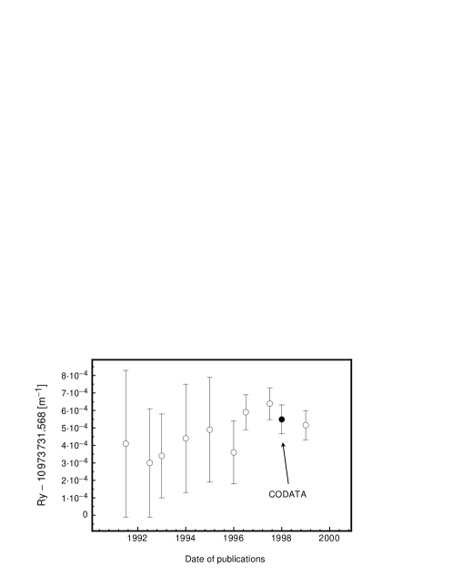
Figure 3: Recent progress in the determination of the Rydberg constant (mainly at MPQ and LKB)

Some other fundamental constants can also be determined by means of laser spectroscopy. To complete the overview let us mention determination of

• the muon-to-electron mass ratio from three-photon ionization of the ground state of muonium at a resonance point of the two-photon excitation of the $2s$ state sgk60mu ;

• the fine structure constant $\alpha$ derived from the helium fine structure;

• the fine structure constant deduced from Raman recoil spectroscopy of the cesium $D_{1}$ line sgk60chu . For this evaluation a precise value of the absolute frequency of the $D_{1}$ line is also necessary.

3 Optical Measurements and Variation of the Fundamental Constants with Time

After the success with understanding of the electromagnetic, weak and, in part, strong interaction we arrived at some sort of threshold of new physics. Naturally, it is not clear on which front one is most likely to discover new physical phenomena. The present-day attempts to discover new physics are rather a kind of a random search for a hidden treasure. Unfortunately, lacking of theoretical predictions there seems to be no better method up to now. One of few directions of such a search is related to the variation of the fundamental constants with time. There is no common model for such a phenomena, but the accepted picture of the evolution of our universe strongly implies for that. ‘Variation’ means a slow drift or oscillation of parameters of the interaction and particle properties (like their masses). We commonly believe that during a small fraction of the very first second our universe came through a number of phase transitions and the interactions and particles as we know them now did not exist before those transitions. So, philosophically speaking, we have to acknowledge the variation of constants as some kind of trace of the early great changes. Physically speaking, we understand that the critical question for a detection of the variation is the rate at which it occurs, because variation rates of $10^{-10}$ yr^-1 and $10^{-20}$ yr^-1 are not the same. Variation of, e. g. the fine structure constant, at the former limit would have already been detected a few decades ago, while the latter rate will rather be a challenge for physicists in a few decades. Present-day searches are related to a level of $10^{-13}-10^{-15}$ yr^-1, which corresponds to a fractional shift of the constants smaller than than $10^{-3}-10^{-5}$ for the life-time of the universe.

There are a number of possibilities for such a search, but the optical measurements play a specific role, because of their clear interpretation. However, the fact of variation is more important than the accurate interpretation. In the case of a negative result no limitation for a variation can be assigned without a reasonable interpretation. From the theoretical point of view we have to expect simultaneous variations of all coupling constants, masses and magnetic moments. If one wishes to find a solid interpretation, some reduction of all variable quantities to a very few is important. However, nuclear properties are the result of the strong interactions and involve effects, that cannot be calculated. Only optical transitions are completely free from this problem.

Table 1: Comparison of different kinds of searches for a variation of fundamental constants. Here $T$ is a half-period of oscillations and $\Delta t$ is a time separation for a comparison. The Laboratory search contains all laboratory measurements, while Optical transitions are for comparison of only optical transitions. The limitation expected in 1-2 years are also presented.

	Geochemical	Astrophysical	Laboratory	Optical
	study	observation	search	transitions
Oscillation	$\Delta t>T$	$\Delta t>T$	phase - ?	phase - ?
Space	$-$	important	$-$	$-$
Statistics	$-$	essential		$-$
Strong Int.	sensitive	not sensitive	sensitive	not sensitive
$\alpha$	$+$	$+$	$+$	$+$
$m_{e}/m_{p}$	$-$	$+$	$+$	$-$
$g_{p}$	$-$	$+$	$+$	$-$
$g_{n}$	$-$	$-$	$+$	$-$
Limitations	$10^{-17}$ yr-1	$10^{-15}$ yr-1	$10^{-15}$ yr-1	$10^{-13}$ yr-1
In 1-2 years				$10^{-14}$ yr-1

We summarize a comparison of different searches in Table 1 sgk60var . Let us discuss briefly the specific features of the different methods.

• To detect a variation one needs to compare some quantity $A(t)$ measured at time $t$ and $t+\Delta t$. However, the obvious estimation of the variation rate $\Delta A/\Delta t$ is valid only in the case of a slow drift. In the case of oscillations, and such oscillations were suggested because of some astrophysical reasons, the estimate must be rather $\Delta A/T$, where $T$ is the half-period of the oscillation ($\sim 10^{8}$ yr). That makes astrophysical ($\delta t\sim 10^{10}$ yr) and geochemical ($\delta t\sim 2\cdot 10^{9}$ yr) estimates much weaker, while in the case of any laboratory experiments we arrive at the question of the phase of such an oscillation. One sees the laboratory search and a search over time (and space) are two different kinds of experiments and serve different purposes.

• Astrophysical data owe two features different from others. First, we can observe the object separated from us both in space and time as there might be a correlation between time- and space- variations. Secondly, the astrophysical data are hard to interpret on an event-by-event base. They used to be treated statistically and it is necessary to study the correlations of the data.

• Another important question for interpretations is involvement of the strong interactions. In the case of geochemical data that is the main effect and there is no reasonable interpretation of such data at all. In the case of laboratory measurements, the strong interaction is important because of the nuclear magnetic moments (see below).

• We can look only for variations of dimensionless quantities such as a ratio of two frequencies and we need to reduce them to a variation of few dimensionless constants, which are the fine structure constant $\alpha$, electron-to-proton mass ratio, $g$-factors of proton and neutron. That is possible because of two reasons, which are

  • known non-relativistic dependence of any transition frequency on the fundamental constants;

  • the Schmidt model predicts nuclear magnetic moments for odd $Z$;

• Non-relativistic theory in particular predicts (see sgk60var for details), that

  • any gross structure transition frequency depends only on the Rydberg constant ($\sim Ry$);

  • any fine structure transition frequency is proportional to $\alpha^{2}Ry$;

  • any hyperfine structure transition is proportional to $\alpha^{2}(\mu/\mu_{B})Ry$, where $\mu$ is the nuclear magnetic moment and $\mu_{B}$ is the Bohr magneton.

• The Schmidt model predicts the magnetic moment of nuclei with odd mass number $A$ as a result of the spin and orbit contribution of a single nucleon (the remaining protons and neutrons are coupled in pairs and do not contribute). Indeed that is a very rough model, but there is no other way to reduce all magnetic moments to few quantities ($m_{e}/m_{p}$, $g_{p}$, $g_{n}$). The problem of interpretation is now related to the inaccuracy of the Schmidt model because of the strong interaction which is not under control.

The present-day level of limitations is different for various methods and the optical experiments do not look as a good choice in general and in comparison with other laboratory experiments. However, the discussion above explains in part that there is no clear interpretation of the geochemical data and there are some doubts in the astrophysical data. There is a single laboratory result in Table 1 that is better than $10^{-13}$ yr^-1: a comparison of the hyperfine splitting in Rb and Cs sgk60Rb . This experiment could be a search for a variation of $g_{p}$. Such an interpretation is valid only if the Schmidt model can be applied, but unfortunately there are essential deviations from the Schmidt model due to the strong interaction (mainly in Cs). The actual interpretation remains unclear.

We briefly discuss optical laboratory experiments below. The current limitations are quite weak ($\sim 10^{-13}\;{yr}^{-1}$) because most of the results were obtained recently on a level of a fractional uncertainty of $10^{-14}$ (see Table 2). These limitations were obtained either after a short-term monitoring or after a comparison with a previous less accurate result. Future limitations based on reproduction of the recent experiments in 2000-2001 must easily deliver limitations better by an order of magnitude.

Table 2: Some results of recent precision optical measurements (H, $1s-2s$, ⁴⁰Ca, ${}^{3}P_{1}-{{}^{1}}S_{0}$, ${}^{115}{\rm In}^{+}$, $5s^{2}{{}^{1}}S_{0}-5s5p{{}^{3}}P_{0}$, ${}^{171}{\rm Yb}^{+}$, $6s^{2}{{}^{2}}S_{1/2}-5d^{2}{{}^{2}}D_{3/2}$, ${}^{199}{\rm Hg}^{+}$, ${}^{2}S_{1/2}-{{}^{2}}D_{5/2}$), their fractional uncertainty $\delta$ and their sensitivity to a variation of the fine structure constant $\kappa=\partial\ln{F_{rel}(\alpha)}/\partial\ln{\alpha}$

Atom	Frequency	Place and date	$\delta$	$\kappa$
	[Hz]	of measurement	[$10^{-14}$]	sgk60Fla
H	2 466 061 413 187 103 (46)	MPQ, 1999, sgk601s2s	1.8	0.00
Ca	455 986 240 494 158 (26)	NIST, 2000, sgk60NIST	5.7	0.03
${\rm In}^{+}$	1 267 402 452 899 920(230)	MPQ, 1999, sgk60In	18	0.21
${\rm Yb}^{+}$	688 358 979 309 312  (6)	PTB, 2001, sgk60PTB	0.9	1.03
${\rm Hg}^{+}$	1 064 721 609 899 143 (10)	NIST, 2000, sgk60NIST	0.9	-3.18

Since all the transitions in Table 2 are related to the gross structure one could wonder how to obtain any information about a variation of the fine structure constant if all of them are proportional (in the non-relativistic approximation) to the Rydberg constant. The signal is due to the relativistic corrections. Their importance (for the hyperfine structure) was first pointed out in sgk60Pre and they were later calculated for a bunch of the optical transitions in sgk60Fla . The transition frequency is now equal to $c\,Ry\,F_{\rm rel}(\alpha)$ and a non-trivial relativistic factor $F_{\rm rel}(\alpha)$ is a key point to look for a variation of the fine structure constant by optical means. The sensitivity $\kappa=\partial\ln{F_{rel}(\alpha)}/\partial\ln{\alpha}$ to a variation of $\alpha$ is given in Table 2 accordingly to sgk60Fla .

A comparison of two optical frequencies can be performed directly (like e.g. an Hg-Ca comparison at NIST sgk60NIST ) or indirectly (via a comparison of both frequency to cesium standard).

A direct comparison of two distinct optical frequencies is now possible using the newly developed femtosecond frequency chains. This approach has the advantage of a high short-term stability as compared with cesium standard. This allows for a simple time structure of the experiment sgk60var with a few direct comparisons. A comparison with cesium often involves some secondary standard with a high short-term stability. Such a clock being an artefact that is not related to any transition should involve an unknown drift with time as the constants are drifting. Their short time stability cannot be actually proved. A common reason for a statement on the good short-time stability of such a standard (like a hydrogen maser for example) is that the scattering of their frequencies with time is small. But there is no idea about a possible common mode rejection. The stronger reason to believe in a good short term stability is a comparison between different clocks. But still there might be a common mode rejection as it should be the case for a variation of the constants. A direct comparison of two optical transitions allows to avoid this problem and offers a new opportunity to securely derive a limitation for a variation of the fine structure constant or maybe even to detect such a variation.

4 Summary

Nowadays, optical spectroscopy of atoms provides an essential input for the determination of the fundamental physical constants, including the most accurately known fundamental constant, the Rydberg constant, which plays an important role in atomic physics. The so-called atomic unit of frequency and energy are related to this constant being $c\cdot Ry$ and $h\cdot c\cdot Ry$ respectively. A definition of the second, attractive from a general point of view, could be based on a fixed value of the Rydberg constant. This would be practically acceptable after the following steps are achieved:

• the completion of a frequency chain that connects the optical with microwave domain and, at the same time allows for a comparison of any optical transition with the $1s-2s$ frequency on in hydrogen (done at MPQ sgk60chain and used now also at NIST, JILA, PTB);

• accurate measurement of the $1s-2s$ transition (done at MPQ sgk601s2s with an accuracy compatible with any other optical transition but not yet competitive with cesium and rubidium fountain clocks);

• proper QED theory of the Lamb shift (essentially developed within the last decades but it still needs more progress);

• determination of the proton charge radius (not known with sufficient accuracy, but a promising experiment is in progress sgk60PSI ).

The hydrogen atom was a candidate for the primary frequency standard in the 1960ies because of the hyperfine splitting, but this attempt failed for a number of reasons. Now it is time for a strong competition of new frequency standards and the hydrogen atom has its second chance.

Actually there is one more fundamental constant, which is associated with the optical measurements. That is the speed of light which is equal to

$$c=299\,792\,458\;{\rm m/s}$$ (2)

because of the definition of the meter. Despite this constant is fixed by definition there is still an uncertainty related to a practical realization of the meter. The problem is that the second is defined with the help of the cesium hyperfine transition, while the meter is related to the optical domain. The accepted recommendations for its realization is based on optical transitions sgk60met . In the case of any direct application of (2) one meets three sources of uncertainty

• a realization of the second in the microwave domain;

• a realization of the meter in the optical domain;

• a bridge between both realizations to the same transition (i.e. the frequency chain).

After recent progress in frequency chain metrology and a long-term development of the microwave standards, present-day limitations come mainly from the optical standards, which however are developing in a very promising way.

The old-fashion frequency chains, which really presented the state of art in the field just few years ago, appear now as some kind of dinosaur, which should very soon disappear. Those chains are much bigger, much more expensive, much more complicated in construction and in use and at the same time less accurate, than the new frequency-comb chains. The main disadvantage of the old technology was a limited possibility in use. The old chains were designed as a single-problem chain and it was necessary to redesign it with adding some more items to adjust it to new transitions. The new chain provides us with a possibility to measure any optical transitions and some measurements like the cesium $D_{1}$ line for example needed for the determination of the fine structure constant sgk60chu are now a routine problem. The chain offers new horizons for precision optical spectroscopy and we look forward for soon reproductions of recent experiments sgk601s2s ; sgk60NIST ; sgk60PTB which must deliver new secure limitations for a possible variation of the fine structure constant with time on a level of $10^{-14}$ per year.

References

- (1)
- (2) F. Biraben and L. Julien, this volume
- (3) M. Weitz, A. Huber, F. Schmidt-Kaler, D. Leibfried, W. Vassen, C. Zimmermann, K. Pachucki, T. W. Hänsch, L. Julien, and F. Biraben, Phys. Rev. A 52, 26641 (1995)
- (4) M. Niering, R. Holzwarth, J. Reichert, P. Pokasov, Th. Udem, M. Weitz, T. W. Hänsch, P. Lemonde, G. Santarelli, M. Abgrall, P. Laurent, C. Salomon, and A. Clairon, Phys. Rev. Lett. 84, 5496 (2000)
-
(5)
J. Reichert, M. Niering, R. Holzwarth, M. Weitz, Th. Udem, and T. W. Hänsch, Phys. Rev. Lett. 84, 3232 (2000);
R. Holzwarth, Th. Udem, T. W. Hänsch, J. C. Knight, W. J. Wadsworth, and P. St. J. Russell, Phys. Rev. Lett. 85, 2264 (2000) - (6) S. A. Diddams, D. J. Jones, J. Ye, S. T. Cundiff, J. L. Hall, J. K. Ranka, R. S. Windeler, R. Holzwarth, Th. Udem, and T. W. H nsch, Phys. Rev. Lett. 84, 5102 (2000)
- (7) Th. Udem and A. Ferguson, this volume
- (8) S. G. Karshenboim, in Atomic Physics 17 (AIP conference proceedings 551) Ed. by E. Arimondo et al. AIP, 2001, pp. 238–253.
- (9) S. G. Karshenboim, F. S. Pavone, F. Bassani, M. Inguscio and T. W. Hänsch. Hydrogen atom: Precision physics of simple atomic systems (Springer, Berlin, Heidelberg, 2001)
- (10) A. Huber, Th. Udem, B. Gross, J. Reichert, M. Kourogi, K. Pachucki, M. Weitz and T. W. Hänsch, Phys. Rev. Lett. 80, 468 (1998)
- (11) C. Schwob, L. Jozefowski, B. de Beauvoir, L. Hilico, F. Nez, L. Julien and F. Biraben, Phys. Rev. Lett. 82 (1999) 4960.
- (12) S. G. Karshenboim, JETP 79, 230 (1994); Z. Phys. D 39, 109 (1997).
- (13) S. G. Karshenboim, JETP 76, 541 (1993)
- (14) M. I. Eides, H. Grotch and V. A. Shelyuto, Phys. Rep. 342 (2001) 63.
- (15) S. G. Karshenboim, Can. J. Phys. 77, 241 (1999)
- (16) P. J. Mohr and B. N. Taylor, Rev. Mod. Phys. 72, 351 (2000)
- (17) K. Jungmann, in sgk60h2 , pp. 81–102
- (18) J. M. Hensley, A. Wicht, B. C. Young, and S. Chu , in Atomic Physics 17 (AIP conference proceedings 551) Ed. by E. Arimondo et al. AIP, 2001, pp. 43–57
- (19) S. G. Karshenboim, Can. J. Phys. 78, 639 (2000)
- (20) C. Salomon, Y. Sortais, S. Bize, M. Abgrall, S. Zhang, C. Nicolas, C. Mandache, P. Lemonde, P. Laurent, G. Santarelli, A. Clairon, N. Dimarcq, P. Petit, A. Mann, A. Luiten, and S. Chang, in Atomic Physics 17 (AIP conference proceedings 551) Ed. by E. Arimondo et al. AIP, 2001, pp. 23–40
- (21) Th. Udem, S. A. Diddams, K. R. Vogel, C. W. Oates, E. A. Curtis, W. D. Lee, W. M. Itano, R. E. Drullinger, J. C. Bergquist, and L. Hollberg, Phys. Rev. Lett. 86, 4996 (2001)
- (22) J. von Zanthier; Th. Becker, M. Eichenseer, A. Yu. Nevsky, Ch. Schwedes, E. Peik, H. Walther, R. Holzwarth, J. Reichert, Th. Udem, T. W. Hänsch, P. V. Pokasov, M. N. Skvortsov, and S. N. Bagayev, Opt. Lett. 25 (2000) 1729
- (23) J. Stenger, Ch. Tamm, N. Haverkamp, S. Weyers, and H. R. Telle, e-print physics/0103040
- (24) J. D. Prestage, R. L. Tjoelker, and L. Maleki, Phys. Rev. Lett. 74, 3511 (1995)
- (25) V. A. Dzuba, V. V. Flambaum, and J. K. Webb, Phys. Rev. A 59, 230 (1999); V. A. Dzuba and V. V. Flambaum, Phys. Rev. A 61, 034502 (2000).
- (26) R. Pohl, F. Biraben, C.A.N. Conde, C. Donche-Gay, T.W. Hänsch, F.J. Hartmann, P. Hauser, V.W. Hughes, O. Huot, P. Indelicato, P. Knowles, F. Kottmann, Y.-W. Liu, V.E. Markushin, F. Mulhauser, F. Nez, C. Petitjean, P. Rabinowitz, J.M.F. dos Santos, L.A. Schaller, H. Schneuwly, W. Schott, D. Taqqu, and J.F.C.A. Veloso, in sgk60h2 , pp. 454–466
- (27) T. J. Quinn, Metrologia 30, 523 (1993); 36, 211 (1999)