Measurement of the forbidden $\bm{6s^{2}\,{}^{1}S_{0}\rightarrow 5d6s\;^{3}D_{1}}$ magnetic-dipole transition amplitude in atomic ytterbium

Abstract

We report on a measurement of a highly forbidden magnetic-dipole transition amplitude in ytterbium using the Stark-interference technique. This amplitude is important in interpreting a future parity nonconservation experiment that exploits the same transition. We find $|\langle 5d6s\;^{3}D_{1}|M1|6s^{2}\,{}^{1}S_{0}\rangle|~{}=~{}1.33(6)_{Stat}(20)_{\beta}\times 10^{-4}\mu_{0}$, where the larger uncertainty comes from the previously measured vector transition polarizability $\beta$. The $M1$ amplitude is small and should not limit the precision of the parity nonconservation experiment.

The proposal to measure parity nonconservation (PNC) in the $6s^{2}\,{}^{1}S_{0}\rightarrow 5d6s\,^{3}D_{1}$ transition in atomic ytterbium (Yb) demille95 has prompted both theoretical porsev95 ; das97 and experimental bowers96 ; bowers99 studies. The magnetic-dipole ($M1$) amplitude for this transition is a key quantity for evaluating the feasibility of a PNC-Stark interference experiment as proposed in demille95 . A nonzero $M1$ amplitude coupled with imperfections in the apparatus can lead to systematic uncertainties in a PNC experiment. Here we present the first experimental determination of the magnetic-dipole amplitude for the ${}^{1}S_{0}\rightarrow^{3}D_{1}$ transition. Our method is based on the technique of Stark interference bouchiat74 ; chu77 ; gilbert84 .

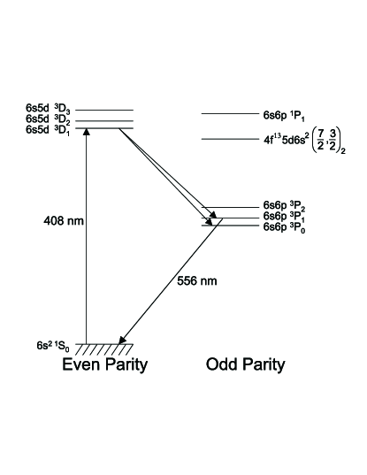
Figure 1: Low-lying energy levels of Yb.

In the absence of external fields, the ${}^{1}S_{0}\rightarrow^{3}D_{1}$ transition (Fig. 1) is highly suppressed. An electric-dipole transition amplitude ${\left[A{\left(E1\right)}\right]}$ is forbidden except for parity mixing effects. A magnetic-dipole transition amplitude is also forbidden because of the s-d nature of the transition. Consequently, a nonzero transition amplitude exists only as a result of configuration mixing and spin-orbit interaction in both the upper and lower states demille95 . There have been no detailed calculations of this amplitude. Reference demille95 gives a rough estimate of $|A{\left(M1\right)}|\lesssim 10^{-4}\mu_{0}$, where $\mu_{0}$ is the Bohr magneton.

In the presence of a static external electric field, ${\mathbf{E}}$, there is a parity-conserving mixing between the even parity ${}^{3}D_{1}$ state and the odd parity states. For a $J=0\rightarrow J=1$ transition, this mixing leads to a Stark-induced electric-dipole transition amplitude given by bouchiat74

$$A{\left(E1_{St}\right)}=i\,\beta\left({\mathbf{E}}\times\bm{\hat{\varepsilon}}\right)_{q},$$ (1)

where $\bm{\hat{\varepsilon}}$ is the direction of the polarization of the laser light, $({\mathbf{E}}\times\bm{\hat{\varepsilon}})_{q}$ is the $q$ component of the vector in the spherical basis, and the vector transition polarizability $\beta$ is a real parameter. The magnitude of $\beta$ was measured bowers99 :

$$|\beta|=2.18(33)\times 10^{-8}{\rm ea_{0}/(V/cm)}.$$ (2)

In an electric field, the transition amplitude is the sum of the Stark-induced $E1$ amplitude and the forbidden $M1$ amplitude. The corresponding transition rate is

$$W \propto {\left|A{\left(E1_{St}\right)}+A{\left(M1\right)}\right|}^{2}$$

$$\approx {\left|A{\left(E1_{St}\right)}\right|}^{2}+2{\rm Re}{\left[A{\left(E1_{St}\right)}{A{\left(M1\right)}^{\ast}}\right]},$$

where we neglect the contribution from ${\left|A{\left(M1\right)}\right|}^{2}$ since $|A{\left(M1\right)}|\ll|A{\left(E1_{St}\right)}|$ with the electric fields and polarization angles used here. The Stark-induced amplitude is proportional to ${\bf E}$. Thus, reversing ${\bf E}$ changes the total transition rate, allowing the interference term to be isolated from the larger terms. The $M1$ amplitude is given by

$$A(M1)=\langle^{3}D_{1},\;M_{J}|M1|^{1}S_{0}\rangle({\bf\hat{k}}\times{\bf\hat{\varepsilon}})_{M_{J}},$$ (4)

where ${\bf\hat{k}}$ is the direction of propagation of the excitation light. Equation 1 implies that only the $M_{J}=\pm 1$ components of the upper state are excited by $A(E1_{St})$, where the axis of quantization is chosen along ${\bf E}$. With ${\bf k}$ perpendicular to ${\bf E}$, the sign of the interference term is opposite for the transitions to the $M_{J}=\pm 1$ components, as can be verified by a simple calculation. Thus, in order to observe the effect of the Stark-M1 interference, we apply a magnetic field, ${\bf B}$, allowing us to resolve different magnetic sublevels. For ${\bf B}$ parallel to ${\bf E}$ (Fig. 2) the interference term in the transition probability is proportional to the rotational invariant $({\bf E}\times\bm{\hat{\varepsilon}})\times(\bm{\hat{k}}\times\bm{\hat{\varepsilon}})\cdot\bm{\hat{B}}$.

Comparison of the difference in the transition rate between opposite electric field states to the sum is a measure of the fractional asymmetry $a$, defined as

$$a \equiv {W(E_{+})-W(E_{-})\over W(E_{+})+W(E_{-})}$$ (5)

$$= {2\langle^{3}D_{1},\;M_{J}|M1|^{1}S_{0}\rangle\over\beta E}{{\rm cos}(\theta)\over{\rm sin}(\theta)}M_{J},$$

where $\theta$ is the angle between the dc electric field and the polarization of the excitation light (Fig. 2). The asymmetry increases with decreasing $\theta$ while the dominant signal decreases as ${\rm sin}^{2}(\theta)$. Most of the data was taken at $\theta=\pm 45^{\circ}$, where the interference term is maximal.

Much of the apparatus used in this experiment had been used for the measurement of the Stark-induced transition amplitude and is described in detail in Refs. bowers99 ; bowers98 . A stainless steel oven with a multi-channel nozzle created an effusive beam of Yb atoms inside of a vacuum chamber with a residual pressure of $\approx 5\times 10^{-6}~{}{\rm Torr}$. The oven nozzle collimation resulted in a Doppler width for the $408$-${\rm nm}$ transition of $\approx~{}150~{}{\rm MHz}$. The oven was heated with tantalum wire heaters operating at $\approx 500~{}^{\circ}{\rm C}$ in the rear with the front $\approx 100~{}^{\circ}{\rm C}$ hotter to avoid clogging. Ytterbium has seven stable isotopes with both zero and nonzero nuclear spin (${}^{168}{\rm Yb}$, ${}^{170}{\rm Yb}$, ${}^{172}{\rm Yb}$, ${}^{174}{\rm Yb}$, ${}^{176}{\rm Yb}$, $I=0$; ${}^{171}{\rm Yb}$, $I=1/2$; and ${}^{173}{\rm Yb}$, $I=5/2$). To avoid significant overlap of the optical spectra of the zero-nuclear-spin isotopes and the hyperfine components of the nonzero-nuclear-spin isotopes, an external vane collimator was installed; reducing the Doppler width to $\approx 15~{}{\rm MHz}$. The vane collimator was made by layering $0.076~{}{\rm mm}$ thick sheets of stainless steel foil between $0.94~{}{\rm mm}$ thick stainless steel spacers. The length of the collimator was $5.1~{}{\rm cm}$, providing a collimation angle of $\approx 1^{\circ}$. The width of the collimator was $3.8~{}{\rm cm}$. The collimator was heated using tantalum wire heaters to $\approx 350~{}^{\circ}{\rm C}$ to prevent clogging. The collimator was mounted on a movable platform, allowing precise alignment of the angle of the collimator relative to the atomic beam during the experiment. We estimate an atomic density of $\approx 2~{}\times~{}10^{9}~{}{\rm cm}^{-3}$ in the interaction region.

Approximately $80~{}{\rm mW}$ of laser light at $408~{}{\rm nm}$ excited ytterbium atoms to the ${}^{3}D_{1}$ state in the geometry shown in Fig. 2. The $408$-${\rm nm}$ light was produced by frequency doubling of $\approx 1.2~{}{\rm W}$ of $816$-${\rm nm}$ light from a titanium-sapphire laser (Coherent 899-21) pumped with $\approx 12\;{\rm W}$ from a multi-line argon-ion laser (Sectra Physics 2080). A commercial bow-tie resonator with a Lithium-Triborate crystal (Laser Analytical Systems Wavetrain cw) provided frequency doubling.

A Burle 8850 photomultiplier tube (PMT) monitored the fluorescence in the $6s6p\;^{3}P_{1}\rightarrow 6s^{2}\;{}^{1}S_{0}$ decay channel at $556~{}{\rm nm}$ (Fig. 1). The top electrode had an array of $198$ $0.12~{}{\rm cm}$ diameter holes, allowing the fluorescence to be collected by a Lucite light guide and conducted to the PMT. The presence of the holes in the top field plate reduced the electric field between the plates. This effect was calculated to be less than $1\%$ using a random walk solution to Laplace’s equation buslenko66 . An interference filter with transmission centered at $560~{}{\rm nm}$ with a $10~{}{\rm nm}$ full width at half maximum was placed in front of the photomultiplier tube in order to limit detection of scattered light at $408~{}{\rm nm}$. Approximately $\approx 0.05\%$ of the atoms undergoing a transition were detected, resulting in typical photocathode currents of $10^{4}~{}{\rm e/s}$ on the peak of the resonance for $|{\bf E}|=15~{}{\rm kV/cm}$. The off-resonance background was consistent with the expected PMT dark current and residual scattered light; contributing a noise $\approx 3$ times less than the signal shot noise for $|{\bf E}|=15~{}{\rm kV/cm}$. The laser frequency was scanned $\approx 200~{}{\rm MHz}$ with both increasing and decreasing frequency over the transition and the fluorescence spectrum was recorded with a digital oscilloscope. The scan time each way was typically $1~{}{\rm s}$. A typical single scan is shown in Fig. 3.

Figure 2: Schematic of apparatus.

After the laser was scanned the polarity of the electric field was either switched or left unchanged in accordance to the following pattern: $\;\left(+~{}-~{}-~{}+~{}-~{}+~{}+~{}-\right)$. This pattern was chosen to limit systematic effects associated with drifts in the laser frequency and atomic beam intensity. A bipolar power supply (Spellman CZE1000R), modified so that the polarity was computer controlled, produced the high voltage used in the experiment. The polarity of the top electrode was reversed while the bottom electrode remained grounded. A resistor divider monitored electrode voltage. The magnitude of this voltage changed by $<0.1\%$ with the change in polarity. A delay of $\approx 2~{}{\rm s}$ after each switch allowed the electric field plates to fully charge before the next scan. The stainless steel electric field plates were separated $1.016~{}{\rm cm}$ by Delrin spacers. The typical value of the electric field was $\approx 12~{}{\rm kV/cm}$. After each sequence of E-field switches, the polarity of the magnetic field was switched according to the $\;\left(+\;-\;-\;+\right)$ pattern. The Earth’s magnetic field was reduced to $\lesssim 50~{}{\rm mG}$ with external coils. A pair of in-vacuum coils in a near Helmholtz configuration provided the uniform magnetic field needed for the experiment. A typical magnetic field was $36~{}{\rm G}$. A run consisted of $5$-$10$ sets of $32$ forward and backward laser scans ($8$ E-field switches $\times$ $4$ B-field switches per set) with fixed values of $\theta$, $|E|$, and $|B|$. Periodically $\approx 50$ laser scans were taken with zero magnetic field in order to monitor for changes in the lineshape of the transition due to temperature fluctuations of the oven and collimator.

A temperature stabilized, hermetically sealed Fabry-Perot cavity with a free spectral range of $150~{}{\rm MHz}$ and finesse of $\approx 15$ was used to monitor a portion of the $816$-${\rm nm}$ light. A photodiode monitored the $408$-${\rm nm}$ laser power in order to normalize the signal for power fluctuations. The transmission through the Fabry-Perot and the $408$-${\rm nm}$ laser power were recorded concurrently with the fluorescence signal.

The Fabry-Perot transmission peaks were used to line up the fluorescence spectra of two consecutive laser scans in order to eliminate frequency drift between scans. Two scans at opposite electric fields and the same magnetic field were combined. The sum of the two fluorescence spectra was fit to the function

$$W(E_{+})+W(E_{-}) =$$

$$\zeta(f\left(\nu-c_{1}\right) + f\left(\nu-c_{2}\right))+m\;\nu+b,$$ (6)

where $\nu$ is the frequency of the laser, $c_{1\left(2\right)}$ is the center position of the first (second) peak, $\zeta$ is the amplitude of the peaks, $m$ and $b$ account for any linear background coming from scattered light. The function $f$ was numerically determined from the spectra taken at zero magnetic field. Because the sign of the interference term is opposite for the different magnetic sublevels (see Eq. 5), the spectral dependence of the asymmetry is given by the difference between the $M_{J}=\pm 1$ peaks multiplied by an asymmetry coefficient. The difference between the two spectra was therefore fit to a function whose line shape was constrained by the fit parameters from the sum fit:

$$W(E_{+})-W(E_{-}) =$$

$$a\;\zeta(\;f\left(\nu-c_{1}\right) - f\left(\nu-c_{2}\right))+C,$$ (7)

where $a$ is the asymmetry coefficient given in Eq. 5, and $C$ accounts, at lowest order, for any possible background that may be present in the difference due to a constant offset in the electric field which does not change sign with the electric field switch. Higher order contributions to the line shape from a constant offset in the electric field were analyzed and found to be insignificant in the determination of $a$. Changing the polarity of the magnetic field reverses the sign of $a$ since the resonance frequencies of the magnetic sublevels switch (Eq. 5). Note that the asymmetry coefficient does not depend on the value of $|{\bf B}|$.

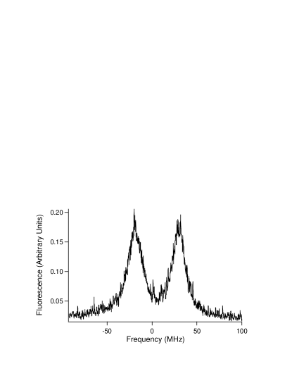
Figure 3: Typical power-normalized, single scan over the $M_{J}~{}=~{}\pm~{}1$ components of the $6s^{2}~{}^{1}S_{0}~{}\rightarrow 5d6s~{}^{3}D_{1}$ transition of ${}^{174}{\rm Yb}$ with $|{\bf E}|=15~{}{\rm kV/cm}$, $\theta=45^{\circ}$, $|{\bf B}|=36~{}{\rm G}$.

The measurements were performed on isotope ${}^{174}{\rm Yb}$ which has a large relative abundance and is spectrally well isolated. The $M1$ transition amplitude was measured in a variety of different field values and configurations. The variation of $E$ was from $5\;{\rm kV/cm}$ to $20\;{\rm kV/cm}$, $\theta$ from $-70^{\circ}$ to $70^{\circ}$, and $B$ from $12\;{\rm G}$ to $84\;{\rm G}$. In addition, data was taken without the external collimator in order to determine possible systematic effects associated with the line-shape modeling or frequency noise. For this data the overlap between the ${}^{174}{\rm Yb}$ and ${}^{173}{\rm Yb}\left(F={5\over 2}\rightarrow F^{\prime}={5\over 2}\right)$ lines was significant and the analysis modified to include effects of this transition.

The effects of misalignments of the fields and imperfect reversals were analyzed analytically and numerically using density matrix formalism. These calculations indicate that systematic effects are significantly smaller than the statistical uncertainty. Possible systematic effects are also severely constrained by confirming the characteristics of the asymmetry. The method of analysis described above is sensitive to asymmetries which reverse sign with ${\bf E}$ and are of opposite sign for the two magnetic sublevels. Equation 5 implies that the sign of the asymmetry should also reverse with ${\bf B}$ and $\theta$. Asymmetries which did not reverse sign with either ${\bf B}$ or $\theta$ were consistent with zero. In addition, the dependence of the magnitude of the asymmetry on the magnitude of ${\bf E}$ and $\theta$ was also verified.

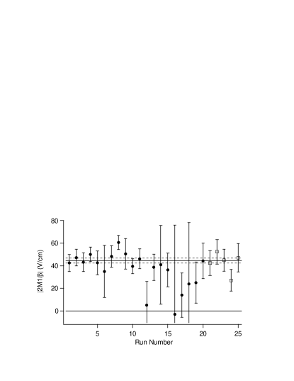
Figure 4: Experimental values of ${\left|{2M1\over\beta}\right|}$. The variation of $E$ was from $5\;{\rm kV/cm}$ to $20\;{\rm kV/cm}$ and $B$ from $12\;{\rm G}$ to $84\;{\rm G}$. The circles (squares) represent data taken with (without) the external collimator. The solid line is the mean and the dashed lines are the statistical error on the mean.

The final value of the $M1$ amplitude is based on data taken on two different days. The data is shown in Fig. 4. The statistical error for each point was estimated from the spread of values obtained for each complete sequence of electric and magnetic field switches within a given configuration. These errors are consistent with the expected limit due to shot noise. Because the errors are estimated from the spread of $5$-$10$ sets, there is some statistical variation in the size of the error assigned to each run. There is additional variation of the errors due to differences in sensitivity for different polarization angles (see Eq. 5) and differences in the amount of data taken in a given configuration. The final result is

$${2\langle^{3}D_{1},\;M_{J}=\pm 1|M1|^{1}S_{0}\rangle\over\beta}=-44.6(21)_{Stat}\;{\rm V/cm}.$$ (8)

This corresponds to an $M1$ amplitude of

$$|{\left\langle{}^{3}D_{1},M_{J}=\pm 1|M1|^{1}S_{0}\right\rangle}|=1.33(6)_{Stat}(20)_{\beta}\times 10^{-4}~{}\mu_{0},$$ (9)

where the second error represents the uncertainty in the determination of $\beta$.

Figure 5: Measured values of ${\left|{2M1\over\beta E}\right|}$ as a function of $|{\bf E}|$. The solid line is the expected dependence from the overall mean and the dashed lines correspond to the errors on the mean.

The measured value of $A(M1)$ agrees with the estimate in Ref. demille95 . This value is $\approx 3$ times larger than the corresponding amplitude in the cesium (Cs) transition where PNC is studied hoffnagle81 ; gilbert84 ; wood97 ; guena98 . However, the expected large enhancement of the PNC amplitude in Yb ($\approx 100$ times larger than in Cs demille95 ) makes the relative size of $A(M1)$ to the PNC amplitude smaller than it is in Cs. An additional suppression of spurious interference between the $M1$ amplitude and the Stark-induced amplitude is possible by using the geometry for the PNC experiment employed in Ref. drell85 . The reported measurement is for the isotopes with zero nuclear spin. The isotopes with nonzero nuclear spin (${}^{171}{\rm Yb}$, $I=1/2$ and ${}^{173}{\rm Yb}$, $I=5/2$) have an additional contribution to the $M1$ amplitude and a small $E2$ amplitude due to hyperfine mixing effects. However, these contributions are estimated to have values $\lesssim 10^{-5}\mu_{0}$ demille95 , and should only lead to small modifications to the present result. These effects will be investigated in future work. The size of the $M1$ amplitude should not limit the precision of a Yb PNC measurement which is in progress in our laboratory.

The authors thank M. Zolotorev and P. A. Vetter for many useful discussions throughout this work and A. Vaynberg for help in constructing the apparatus. E. D. Commins and C. J. Bowers made important contributions to early stages of the work. This work was supported by the NSF, grant $PHY-9877046$.

References

- (1) D. DeMille, Phys. Rev. Lett. 74, 4165 (1995).
- (2) S. G. Porsev, Yu. G. Rakhlina, and M. G. Kozlov, Pis’ma Zh. Éksp. Teor. Fiz. 61, 449 (1995) [JETP Lett. 61, 459 (1995)].
- (3) B.P. Das, Phys. Rev. A 56, 1635 (1997).
- (4) C. J. Bowers, D. Budker, E. D. Commins, D. DeMille, S. J. Freedman, A.-T. Nguyen, S.-Q. Shang, M. Zolotorev, Phys. Rev. A 53, 3103 (1996).
- (5) C. J. Bowers, D. Budker, S. J. Freedman, G. Gwinner, J. E. Stalnaker, and D. DeMille, Phys. Rev. A 59, 3513 (1999).
- (6) M. A. Bouchiat and C. Bouchiat, J. Phys (Paris) 35, 899 (1974); Ibid. 36, 493 (1975).
- (7) S. Chu, E.D. Commins, and R. Conti, Phys. Lett. 60A, 96 (1977).
- (8) S. L. Gilbert, R. N. Watts, and C. E. Wieman, Phys. Rev. A 29, 137 (1984).
- (9) C. J. Bowers, Ph. D. thesis; J. E. Stalnaker, Undergraduate thesis, University of California at Berkeley (1998). (http://socrates.berkeley.edu/budker)
- (10) N.P. Buslenko et al. The Monte Carlo method; the method of statistical trials, ed. by Yu. A. Shreider (Pergamon Press, Oxford, 1966).
- (11) J. Hoffnagle, L. Ph. Roesch, V. L. Telegdi, A. Weis, and A. Zehnder, Phys. Lett. 85A, 143 (1981).
- (12) C. S. Wood, et al. , Science 275, 1759 (1997); Can. J. Phys. 77, 7 (1998).
- (13) J. Guéna, D. Chauvat, Ph. Jacquier, M. Lintz, M. D. Plimmer, and M.A. Bouchiat, Quan. Semiclass. Opt. 10, 733 (1998).
- (14) P. S. Drell and E. D. Commins, Phys. Rev. A 32, 2196 (1985).