$\lambda/4$, $\lambda/8$, and higher order atom gratings via Raman transitions

Abstract

A method is proposed for producing atom gratings having period $\lambda/4$ and $\lambda/8$ using optical fields having wavelength $\lambda$. Counterpropagating optical fields drive Raman transitions between ground state sublevels. The Raman fields can be described by an effective two photon field having wave vector $2{\bf k}$, where ${\bf k}$ is the propagation vector of one of the fields. By combining this Raman field with another Raman field having propagation vector $-2{\bf k}$, one, in effect, creates a standing wave Raman field whose “intensity” varies as $\cos(4{\bf k\cdot r}).$ When atoms move through this standing wave field, atom gratings having period $\lambda/4$ are produced, with the added possibility that the total ground state population in a given ground state manifold can have $\lambda/8$ periodicity. The conditions required to produce such gratings are derived. Moreover, it is shown that even higher order gratings having periodicity smaller than $\lambda/8$ can be produced using a multicolor field geometry involving three (two-photon) Raman fields. Although most calculations are carried out in the Raman-Nath approximation, the use of Raman fields to create reduced period optical lattices is also discussed.

I Introduction

The field of optical coherent transients [1] had at its origin the pioneering work of Kurnit, Abella, and Hartmann on photon echoes [2]. Since that work, Hartmann and coworkers have made a large number of significant contributions in both cw and transient nonlinear spectroscopy. One of us (PRB) had the good fortune to collaborate with his group on problems related to diffractive scattering of atoms in superposition states [3]. There were also a number of spirited discussions on the billiard ball model of photon echoes [4], a model which was somewhat before its time since it is now used commonly in theoretical models of atom interferometers [5]. It is with great pleasure that we participate in this festschrift volume to honor Sven Hartmann.

The first wave of experiments on optical coherent transients, such as photon echoes and free precession [6], involved coherence between different electronic states that are coupled by an optical field. Subsequent experiments, however, such as the stimulated photon echo [7], employed optical fields as a means for creating coherence between ground state sublevels (or a spatial modulation of a single ground state population). Since ground state coherences can have decoherence times approaching seconds, rather than the tens or hundreds of nanoseconds associated with optical transitions, ground state coherence has important applications in atom interferometry and quantum information. There is now an extensive literature on both cw and coherent transient, ground state spectroscopy.

In recent years, both cw and pulsed optical fields have been used to control the center-of-mass motion of atoms. Of particular interest to the current discussion is the possibility of using optical fields having wavelength $\lambda$ to create high-order matter wave gratings having period $\lambda/2n$, where $n$ is a positive integer greater than or equal to $2$ [8]. Such matter wave gratings could serve as efficient scatters of soft x-rays. There have been several schemes proposed for achieving this goal, but most of these schemes involve several atom-field interaction zones. Recently we showed that it is possible to create high-order gratings in a single interaction zone using a set of counterpropagating optical fields having different frequencies [9]. One of the limitations of that work was set by the lifetime of the excited state of the transition. The product of atom-field detunings and excited state lifetime has to be much greater than unity to satisfy certain adiabaticity requirements, and this necessitates the use of large detunings that leads to a corresponding decrease in transition amplitudes.

These problems can be avoided if one replaces the optical transitions with ground-state, Raman transitions. A pair of fields drives transitions from one ground state sublevel to another and acts as an effective two-photon field that is the analogue of the single field that drives an optical transition. In analogue with the optical case, the two-photon field leads to a spatially modulated Raman coherence, but not to a spatially modulated population of the ground state sublevels[10]. However, a pair of such two-photon fields, acting as a Raman standing wave field, leads to ground state gratings having period $\lambda/4$. With a proper choice of field polarization and initial conditions, the population density in these systems can have period $\lambda/8$, even if the overall period of the matter wave gratings (including the dependence on internal states) has periodicity $\lambda/4$. Moreover, a field geometry involving three pairs of fields can be used to produce gratings having period $\lambda/4n$, where $n$ is a positive integer greater than 2. We first describe the method for producing $\lambda/4$ periodicity and then discuss briefly how to extend this method to produce higher-order gratings. The possibility of creating optical lattices having period $\lambda/4n$ using these techniques is explored.

II Basic Formalism

Consider an atom interacting with a field that consists of a sum of traveling wave fields. The total electric field vector is given by

$${\bf E}\left({\bf r,}t\right)=\frac{1}{2}E_{j}{\bf e}_{j}\exp\left(i{\bf k}_{j}\cdot{\bf r}-i\Omega_{j}t\right)+c.c.,$$ (1)

where $E_{j},$ ${\bf e}_{j},$ ${\bf k}_{j}\$and $\Omega_{j}$ are the amplitude, polarization, wave vector and frequency of wave $j$; there is a summation convention implicit in Eq. (1) and below in which repeated indices appearing on the right-hand side of an equation are to be summed over, except if these indices also appear on the left-hand side of the equation. The field (1) drives transitions between a ground-state manifold characterized by quantum numbers $L_{G}$ (total orbital angular momentum), $S$ (total spin angular momentum), $J_{G}$ (coupling of $L_{G}$ and $S_{G}$), $I$ (total nuclear spin angular momentum), $G$ (coupling of $J_{G}$ and $I$), $m_{g}$ (Zeeman quantum number), and excited-state manifold characterized by quantum numbers $L_{H}$, $S,$ $J_{H},$ $I,$ $H,$ $m_{h}.$ In the resonant or rotating-wave approximation the atomic state probability amplitudes evolve as

$$i\dot{a}_{Hm_{h}} = \exp\left(-i\Delta_{Hm_{h},Gm_{g}}^{\left(j\right)}t+i{\bf k}_{j}\cdot{\bf r}\right)\chi_{Hm_{h},Gm_{g}}^{\left(j\right)}a_{Gm_{g}}-\gamma_{H}a_{Hm_{h}}/2,$$ (3)

$$i\dot{a}_{Gm_{g}} = \exp\left(i\Delta_{Hm_{h},Gm_{g}}^{\left(j\right)}t-i{\bf k}_{j}\cdot{\bf r}\right)\left[\chi_{Hm_{h},Gm_{g}}^{\left(j\right)}\right]^{\ast}a_{Hm_{h}},$$ (4)

where

$$\chi_{Hm_{h},Gm_{g}}^{\left(j\right)}=\left(-1\right)^{\nu}\chi_{HG}^{\left(j\right)}e_{-\nu}^{\left(j\right)}\left(2H+1\right)^{-1/2}\left\langle Gm_{g},1\nu|Hm_{h}\right\rangle,$$ (5)

is a Rabi frequency,

$\displaystyle\Delta_{Hm_{h},Gm_{g}}^{\left(j\right)}=\Omega_{j}-\omega_{Hm_{h},Gm_{g}}$

is an atom-field detuning,

$\displaystyle\chi_{HG}^{\left(j\right)}=-\mu_{HG}E_{j}/2\hbar$

is a reduced Rabi frequency, $\mu_{HG}$ is the reduced matrix element of the dipole moment operator between states $H$ and $G$, $\gamma_{H}$ is an excited state decay rate, $e_{\nu}^{\left(j\right)}$ are spherical components of the polarization ${\bf e}_{j}$,

$$e_{\pm 1}^{\left(j\right)}=\mp\frac{e_{x}^{\left(j\right)}\pm e_{y}^{\left(j\right)}}{\sqrt{2}}\text{; \ \ }e_{0}^{\left(j\right)}=e_{z}^{\left(j\right)}$$ (6)

and $\left\langle Gm_{g},1\nu|Hm_{h}\right\rangle$ is a Clebsch-Gordan coefficient.

For far detuned fields $\left(\left|\Delta_{Hm_{h},Gm_{g}}^{\left(j\right)}\right|\gg\gamma_{H},\left|\chi_{HG}^{\left(j\right)}\right|\right)$, one can use a secular approximation, where excited states amplitudes adiabatically follow ground state amplitudes as

$$a_{Hm_{h}}=\exp\left(-i\Delta_{Hm_{h},Gm_{g}}^{\left(j\right)}t+i{\bf k}_{j}\cdot{\bf r}\right)\left(\chi_{Hm_{h},Gm_{g}}^{\left(j\right)}/\Delta_{Hm_{h},Gm_{g}}^{\left(j\right)}\right)a_{Gm_{g}}.$$ (7)

Substituting this expression in Eq. (4) one arrives at the Schrödinger equation for the ground state manifold

$$i\dot{a}_{G^{\prime}m_{g}^{\prime}}=\left\langle G^{\prime}m_{g}^{\prime}\left|V\right|Gm_{g}\right\rangle a_{Gm_{g}},$$ (8)

where $\hbar V$ is a reduced Hamiltonian with matrix elements

$$\left\langle G^{\prime}m_{g}^{\prime}\left|V\right|Gm_{g}\right\rangle=\exp\left[-i\delta_{G^{\prime}m_{g}^{\prime},Gm_{g}}^{\left(jj^{\prime}\right)}t+i{\bf k}_{jj^{\prime}}\cdot{\bf r}\right]A_{G^{\prime}G}^{\left(jj^{\prime}\right)}\left(K\right)\left\langle G^{\prime}m_{g}^{\prime},KQ|Gm_{g}\right\rangle\varepsilon_{Q}^{K}\left(jj^{\prime}\right),$$ (9)

$$\delta_{G^{\prime}m_{g}^{\prime},Gm_{g}}^{\left(jj^{\prime}\right)}=\Omega_{j}-\Omega_{j^{\prime}}-\omega_{G^{\prime}m_{g}^{\prime},Gm_{g}}$$ (10)

is the Raman detuning associated with the two-quantum transition $Gm_{g}\rightarrow G^{\prime}m_{g}^{\prime}$ involving absorption from field $j$ and emission into field $j^{\prime}$,

$$A_{G^{\prime}G}^{\left(jj^{\prime}\right)}\left(K\right)=\left(-1\right)^{G^{\prime}+H+K}\left[\chi_{HG}^{\left(j\right)}\left(\chi_{HG^{\prime}}^{\left(j^{\prime}\right)}\right)^{\ast}/\Delta_{H,G}^{\left(j\right)}\right]\left[\left(2K+1\right)/\left(2G+1\right)\right]^{1/2}\left\{\begin{array}[]{ccc}G&G^{\prime}&K\\ 1&1&H\end{array}\right\},$$ (11)

$\left\{\ldots\right\}$ is a 6-J symbol, and

$$\varepsilon_{Q}^{K}\left(jj^{\prime}\right)=\left(-1\right)^{\nu^{\prime}}e_{\nu}^{\left(j\right)}\left(e_{-\nu^{\prime}}^{\left(j^{\prime}\right)}\right)^{\ast}\left\langle 1\nu,1\nu^{\prime}|KQ\right\rangle$$ (12)

is a tensor coupling vectors ${\bf e}_{j}$ and ${\bf e}_{j^{\prime}}.$ It has been assumed that single photon detuning is much larger than any Zeeman splittings, i.e. $\Delta_{Hm_{h},Gm_{g}}^{\left(j\right)}\approx\Delta_{H,G}^{\left(j\right)}.$

If the single photon detunings are much larger than the excited state hyperfine splitting, $\Delta_{H,G}^{\left(j\right)}\approx\Delta_{J_{H},G}^{\left(j\right)}$, one can sum over $H$ to arrive at

$$A_{G^{\prime}G}^{\left(jj^{\prime}\right)}\left(K\right) = \left(-1\right)^{G^{\prime}+J_{G^{\prime}}+J_{G}+J_{H}+I}\left[\chi_{J_{H}J_{G}}^{\left(j\right)}\left(\chi_{J_{H}J_{G^{\prime}}}^{\left(j^{\prime}\right)}\right)^{\ast}/\Delta_{J_{H},G}^{\left(j\right)}\right]\left[\left(2K+1\right)\left(2G^{\prime}+1\right)\right]^{1/2}$$ (18)

$$\times\left\{\begin{array}[]{ccc}J_{G}&J_{G^{\prime}}&K\\ 1&1&J_{H}\end{array}\right\}\left\{\begin{array}[]{ccc}J_{G^{\prime}}&I&G^{\prime}\\ G&K&J_{G}\end{array}\right\}.$$

Finally, if the single photon detunings are larger than the excited state fine structure intervals, $\Delta_{J_{H},G}^{\left(j\right)}\approx\Delta_{L_{H},G}^{\left(j\right)},$ one finds

$$A_{G^{\prime}G}^{\left(jj^{\prime}\right)}\left(K\right) = \left(-1\right)^{G^{\prime}+J_{G^{\prime}}+J_{G}+I+S+L_{H}+K}\left[\chi_{L_{H}L_{G}}^{\left(j\right)}\left(\chi_{L_{H}L_{G}}^{\left(j^{\prime}\right)}\right)^{\ast}/\Delta_{L_{H},G}^{\left(j\right)}\right]\left[\left(2K+1\right)\left(2G^{\prime}+1\right)\left(2J_{G}+1\right)\left(2J_{G^{\prime}}+1\right)\right]^{1/2}$$ (26)

$$\times\left\{\begin{array}[]{ccc}L_{G}&S&J_{G^{\prime}}\\ J_{G}&K&L_{G}\end{array}\right\}\left\{\begin{array}[]{ccc}L_{G}&L_{G}&K\\ 1&1&L_{H}\end{array}\right\}\left\{\begin{array}[]{ccc}J_{G^{\prime}}&I&G^{\prime}\\ G&K&J_{G}\end{array}\right\},$$

In the latter case, for alkali metal atoms having $L_{G}=0,$ only $K=0$ contributes to the sum. As a consequence, one cannot couple different ground state sublevels if the single photon detunings are larger than excited state fine structure splitting. The two-photon Raman field acts as a scalar in this case.

III Atom gratings

Equations (8), with the effective Hamiltonian (9) are the starting point for a wide class of problems involving both $cw$ and transient ground state spectroscopy. If one diagonalizes the effective Hamiltonian (9), he obtains the spatially-dependent optical potentials that characterize this atom field interaction. We will return to this point in the Discussion. It has been assumed implicitly in Eq. (8) that ${\bf r}$, the atomic center-of-mass coordinate, is a classical variable; however, it is possible to generalize these equations to allow for quantization of the center-of-mass motion by addition of a term $\hbar\nabla^{2}a_{G^{\prime}m_{g}^{\prime}}/2M$ ($M$ is an atomic mass) to the left hand side of Eq. (8). In this paper, we analyze problems in which atoms are subjected to a radiation pulse whose duration is sufficiently short to justify neglect of this kinetic energy term (Raman-Nath approximation). The radiation pulse can occur in the laboratory frame or in the atomic rest frame (e.g. when an atomic beam passes through a field interaction zone). Following the interaction region, the atomic wave function evolves freely and the kinetic energy term must be included, leading to such effects as atom focusing and Talbot rephasing, but we concentrate here on the evolution of the wavefunction only in the field interaction region.

Even with the simplification afforded by the Raman-Nath approximation, Eqs. (8) must be solved numerically, in general. To illustrate the relevant physics, we consider two limiting cases for which an analytic solution can be obtained, $\sigma_{+},\sigma_{-}$ radiation and $\pi$-polarized radiation.

A Basic formalism

Let us assume that there are a number of ground state manifolds, $G,$ $G^{\prime}$, $G^{\prime\prime}$, etc., and that a pair of optical fields comprising our effective two-photon field drives transitions from sublevels in one manifold to sublevels in the same or other manifolds. The key point in considering these Raman transitions is a directionality in which one couples the initial state (or states) to the final states by absorption from field 1 and emission into field 2 but not by absorption from field 2 and emission into field 1. Similarly, one couples the final states to the initial states by absorption from field 2 and emission into field 1 but not by absorption from field 1 and emission into field 2. Some simple examples will illustrate how this feat can be accomplished. Suppose first that there is a single ground state manifold having $G=1$, with the initial state having $m_{g}=-1$ and the final state having $m_{g}=1$. By choosing the first field to have $\sigma_{+}$ polarization and the second field to have $\sigma_{-}$ polarization, the first field couples only the initial state to the excited states and the second field only the final state to the excited states. Alternatively, consider initial states in the $G$ manifold and final states in the $G^{\prime}$ manifold with $\left|\omega_{G^{\prime}G}\right|\tau\gg 1$, where $\tau$ is the interaction time. If one chooses the first field to have frequency $\Omega_{11}$ and the second field to have frequency $\Omega_{21}$ such that $\left[\left(\Omega_{11}-\Omega_{21}\right)-\omega_{G^{\prime}G}\right]\tau\lesssim 1$ but $\left|\Omega_{11}-\Omega_{21}\right|\tau\gg 1,$ then the transition from initial to final states can be realized only by absorption from field 1 and emission into field 2 (and not by from absorption from field 2 and emission into field 1).

Consequently, we assume that there are two sets of fields having frequencies $\Omega_{1j}$ $\left(j=1,2\ldots n\right)$ and $\Omega_{2j}$ $\left(j=1,2\ldots n\right)$ from which we can form our required pairs of two-photon field operators using one field having frequency $\Omega_{1j}$ and the second field having frequency having $\Omega_{2j}.$ To simplify matters, it is assumed that $\left(\Omega_{1j}-\Omega_{2j}\right)=$constant, independent of $j.$ By a proper choice of field frequencies or polarizations, two-photon field operators formed from any other combination of fields are assumed to contribute negligibly to the Raman transition amplitude of interest. Of course there will be two photon operators formed by using each field with itself that couples any ground state level to itself (and possibly to other, degenerate ground state sublevels within the same manifold). These operators constitute generalized light shift operators and must be accounted for in the theory, but are not spatially dependent.

In a field interaction representation defined by

$$a_{Gm_{g}}=e^{i\delta t/2}\tilde{a}_{Gm_{g}},\text{ }a_{G^{\prime}m_{g}^{\prime}}=e^{-i\delta t/2}\tilde{a}_{G^{\prime}m_{g}^{\prime}}$$ (27)

where

$$\delta=\Omega_{1j}-\Omega_{2j}-\omega_{G^{\prime}G},$$ (28)

one arrives at the evolution equations for the state amplitudes

$$i\dot{a}_{Gm_{g}} = \left[\frac{\delta}{2}\delta_{m_{g}m_{g}^{\prime}}+A_{GG}^{\left(\alpha j,\alpha j\right)}\left(K\right)\left\langle Gm_{g},KQ|Gm_{g}^{\prime}\right\rangle\varepsilon_{Q}^{K}\left(\alpha j,\alpha j\right)\right]a_{Gm_{g}^{\prime}}$$ (31)

$$+e^{-i{\bf q}_{j}\cdot{\bf r}}\left[A_{G^{\prime}G}^{\left(1j,2j\right)}\left(K\right)\left\langle G^{\prime}m_{g}^{\prime},KQ|Gm_{g}\right\rangle\varepsilon_{Q}^{K}\left(1j,2j\right)\right]^{\ast}a_{G^{\prime}m_{g}^{\prime}},$$

$$i\dot{a}_{G^{\prime}m_{g}^{\prime}} = \left[-\frac{\delta}{2}\delta_{m_{g}^{\prime}m_{g}}+A_{G^{\prime}G^{\prime}}^{\left(\alpha j,\alpha j\right)}\left(K\right)\left\langle G^{\prime}m_{g}^{\prime},KQ|G^{\prime}m_{g}\right\rangle\varepsilon_{Q}^{K}\left(\alpha j,\alpha j\right)\right]a_{G^{\prime}m_{g}}$$ (33)

$$+e^{i{\bf q}_{j}\cdot{\bf r}}A_{G^{\prime}G}^{\left(1j,2j\right)}\left(K\right)\left\langle G^{\prime}m_{g}^{\prime},KQ|Gm_{g}\right\rangle\varepsilon_{Q}^{K}\left(1j,2j\right)a_{Gm_{g}},$$

where

$${\bf q}_{j}={\bf k}_{1j}-{\bf k}_{2j},$$ (34)

the tildes have been dropped, and the sum over $\alpha$ is from 1 to 2. The notation has been changed slightly in that the superscript ($j,j^{\prime}$) on the $A$’s in Eqs. (11,18,26) have been replaced by ($\alpha j,\alpha^{\prime}j$).

Consider now the limiting case where there are only two pairs of Raman fields $j=1,2$ (see Fig. 1).Looking for a solution to Eqs. (28) of the form

$\displaystyle a_{Gm_{g}}=\exp\left[-i{\bf Q\cdot r/2}\right]\tilde{a}_{Gm_{g}},\text{ \ }a_{G^{\prime}m_{g}}=\exp\left[i{\bf Q\cdot r/}2\right]\tilde{a}_{G^{\prime}m_{g}}$

$\left[{\bf Q=}\left({\bf q}_{1}+{\bf q}_{2}\right)/2\right]$ and dropping the tildes, one gets

$$i\dot{a}_{Gm_{g}} = \left[\frac{\delta}{2}\delta_{m_{g}m_{g}^{\prime}}+A_{GG}^{\left(\alpha j,\alpha j\right)}\left(K\right)\left\langle GK,m_{g}Q|Gm_{g}^{\prime}\right\rangle\varepsilon_{Q}^{K}\left(\alpha j,\alpha j\right)\right]a_{Gm_{g}^{\prime}}+V_{m_{g}^{\prime}m_{g}}^{\ast}a_{G^{\prime}m_{g}^{\prime}},$$ (36)

$$i\dot{a}_{G^{\prime}m_{g}^{\prime}} = \left[-\frac{\delta}{2}\delta_{m_{g}^{\prime}m_{g}}+A_{G^{\prime}G^{\prime}}^{\left(\alpha j,\alpha j\right)}\left(K\right)\left\langle G^{\prime}K,m_{g}^{\prime}Q|G^{\prime}m_{g}\right\rangle\varepsilon_{Q}^{K}\left(\alpha j,\alpha j\right)\right]a_{G^{\prime}m_{g}}+V_{m_{g}^{\prime}m_{g}}a_{Gm_{g}},$$ (37)

where

$$V_{m_{g}^{\prime}m_{g}}=e^{i{\bf q\cdot r}}A_{G^{\prime}G}^{\left(11,21\right)}\left(K\right)\left\langle G^{\prime}m_{g}^{\prime},KQ|Gm_{g}\right\rangle\varepsilon_{Q}^{K}\left(11,21\right)+e^{-i{\bf q\cdot r}}A_{G^{\prime}G}^{\left(12,22\right)}\left(K\right)\left\langle G^{\prime}m_{g}^{\prime},KQ|Gm_{g}\right\rangle\varepsilon_{Q}^{K}\left(12,22\right)$$ (38)

and

$${\bf q=}\left({\bf q}_{1}-{\bf q}_{2}\right)/2=\left({\bf k}_{11}-{\bf k}_{21}-{\bf k}_{12}+{\bf k}_{22}\right)/2{\bf.}$$ (39)

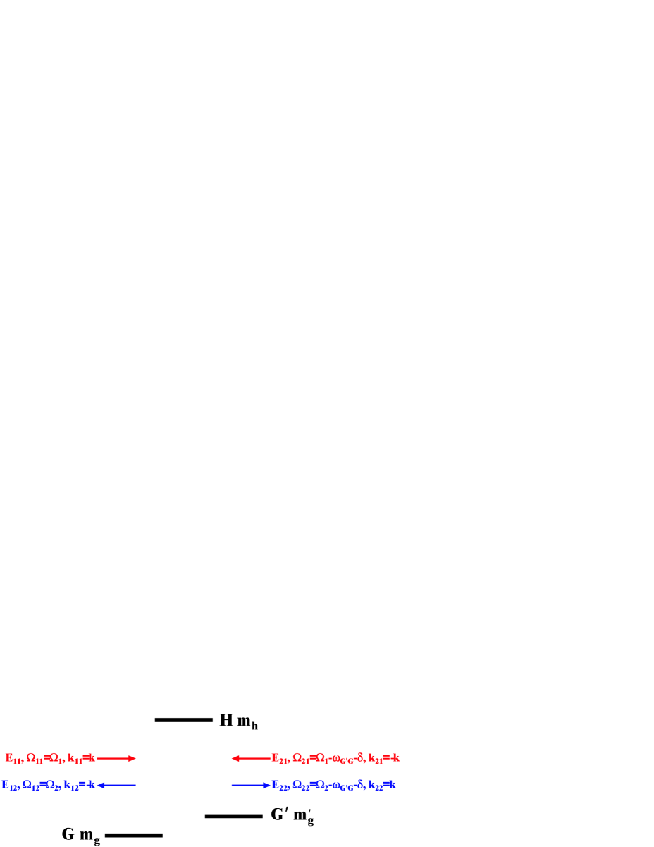
FIG. 1.: Basic Raman configuration.

One sees that, under the transformation

$${\bf\hat{q}\cdot r}\rightarrow{\bf\hat{q}\cdot r}+\pi/q,$$ (40)

the off-diagonal elements of the reduced Hamiltonian change their signs. If the initial density matrix contains no $G-G^{\prime}$ coherence ( for $G\neq G^{\prime}$), the final state populations are unaffected by this sign change. As a consequence atomic state population gratings are produced having period

$$d_{g}=2\pi/\left|{\bf k}_{11}-{\bf k}_{21}-{\bf k}_{12}+{\bf k}_{22}\right|.$$ (41)

For ${\bf k}_{1}=-{\bf k}_{1^{\prime}}=-{\bf k}_{2}={\bf k}_{2^{\prime}}={\bf k}$ one gets a $\lambda/4$-period atom grating. In the case of off-resonant fields, when the $a_{G^{\prime}m_{g}^{\prime}}$ state amplitude can be adiabatically eliminated, it follows immediately from Eqs. (III A) that the periodicity of the $a_{Gm_{g}}$ state amplitude is $\pi/q,$ reflecting the fact that atom phase gratings having this periodicity are produced in the off-resonant case.

B $\sigma_{+},\sigma_{-}$ radiation

Let us assume that there is a single ground state manifold having angular momentum $G=1.$ Atoms interact with a pair of two-photon fields. The first two-photon field consists of a field {$E_{11}=E,$ ${\bf k}_{11}={\bf k=}k{\bf\hat{z}},$ $\Omega_{11}=\Omega_{1}\}$ which is polarized $\sigma_{+}$ and a field {$E_{21}=E,$ ${\bf k}_{21}=-{\bf k},$ $\Omega_{21}=\Omega_{1}-\delta\}$ which is polarized $\sigma_{-}$. This two-photon field is characterized by a polarization tensor

$$\varepsilon_{Q}^{K}\left(11,21\right)=-\delta_{K,2}\delta_{Q,-2}$$ (42)

and drives transitions between the $m_{g}=\pm 1$ sublevels. The second two-photon field has the same polarization and field amplitudes, opposite propagation vectors, ${\bf k}_{12}=-{\bf k}_{22}=-{\bf k,}$ and a carrier frequency $\Omega_{12}=\Omega_{2}$, which is chosen in a manner to ensure that $\left|\Omega_{1}-\Omega_{2}\right|\tau\gg 1$, where $\tau$ is the pulse duration.

For this field polarization, Eqs. (8), in the field interaction representation $a_{1-1}=e^{i\delta t/2}\tilde{a}_{1-1},$ $a_{11}=e^{-i\delta t/2}\tilde{a}_{11},$ reduce to

$$i\dot{a}_{1-1} = \left[\frac{\delta}{2}+S\right]a_{1-1}+T^{\ast}\cos\left(2kz\right)a_{11},$$ (44)

$$i\dot{a}_{11} = \left[-\frac{\delta}{2}+S\right]a_{11}+T\cos\left(2kz\right)a_{1-1},$$ (45)

where the tildes are dropped,

$$S=A_{11}^{\left(\alpha j,\alpha j\right)}\left(K\right)\left\langle 11,K0|11\right\rangle\varepsilon_{0}^{K}\left(\alpha j,\alpha j\right)$$ (46)

is a light shift, and

$$T=-2\left(3/5\right)^{1/2}A_{11}^{\left(11,21\right)}\left(2\right)$$ (47)

is a coupling strength.

If the atoms are prepared in state $m_{g}=-1$ using optical pumping and if $\delta=0$, then a perturbative solution of Eqs. (III B) yields

$$\left|a_{11}\right|^{2}=\left|\int T(t)dt\right|^{2}\cos^{2}\left(2kz\right)$$ (48)

where the integral is over the pulse duration. The final state population is modulated with period

$$d_{g}=\lambda/4.$$ (49)

C $\pi-$polarized radiation

We now return to Raman transitions between $G$ and $G^{\prime}$ manifolds. For $\pi$-polarized fields $\left(e_{\nu}^{\left(j\right)}=e_{\nu}^{\left(j^{\prime}\right)}=\delta_{\nu 0}\right),$ linearly polarized along the $z$ axis and propagating in the ${\bf\hat{x}}$ direction,

$$\varepsilon_{Q}^{K}\left(jj\right)=\varepsilon_{Q}^{K}\left(jj^{\prime}\right)=3^{-1/2}\left(-\delta_{K0}+2^{1/2}\delta_{K2}\right)\delta_{Q0},$$ (50)

and one is led to a collection of independent two-level transitions characterized by quantum numbers $\left(Gm_{g},G^{\prime}m_{g}\right)$. Equations (III A) reduce to

$$i\dot{a}_{Gm_{g}} = \left(\frac{\delta}{2}+S_{G}\right)a_{Gm_{g}}+\left(e^{-iqx}T_{1}^{\ast}+e^{iqx}T_{2}^{\ast}\right)a_{G^{\prime}m_{g}},$$ (52)

$$i\dot{a}_{G^{\prime}m_{g}} = \left(-\frac{\delta}{2}+S_{G^{\prime}}\right)a_{G^{\prime}m_{g}}+\left(e^{iqx}T_{1}+e^{-iqx}T_{2}\right)a_{Gm_{g}},$$ (53)

where $S_{G}$ is the light shift of the initial state given by

$$S_{G}=-3^{-1/2}A_{GG}^{\left(\alpha j,\alpha j\right)}\left(0\right)+\left(1-\delta_{G,1/2}\right)\left[1.5\left(2G-1\right)G\left(G+1\right)\left(2G+3\right)\right]^{-1/2}\left[3m_{g}^{2}-G\left(G+1\right)\right]A_{GG}^{\left(\alpha j,\alpha j\right)}\left(2\right),$$ (55)

$S_{G^{\prime}}$ is the light shift of the final state, obtained from (55) by the replacement $G\rightarrow G^{\prime},$ and

$$T_{j}=3^{-1/2}\left[-\delta_{G^{\prime}G}A_{G^{\prime}G}^{\left(1j,2j\right)}\left(0\right)+2^{1/2}\left\langle G^{\prime}m_{g},20|Gm_{g}\right\rangle A_{G^{\prime}G}^{\left(1j,2j\right)}\left(2\right)\right]$$ (55)

is an effective Rabi frequency for the Raman transition involving absorption from field $1j$ and emission into field $2j$. For ${\bf k}_{11}=-{\bf k}_{11}=-{\bf k}_{21}={\bf k}_{22}={\bf k,}$ and for equal Rabi frequencies and light shifts, Eqs. (50) reduce to (III B), so that the solutions discussed below are also relevant for $\sigma_{+}\sigma_{-}$ radiation.

Since the field envelopes are time dependent, the light shifts and Rabi frequencies are also time dependent, implying that Eq. (50) must be solved numerically, in general. Equations (50) can be solved analytically for rectangular pulses. For pulses having arbitrary shape Eqs. (50) can be solved analytically in two limiting cases, which we refer to as ”resonant” and ”far-detuned”.

In the resonant case, one takes $\delta=0$ and chooses the ratio of the Rabi frequencies in such a way that $S_{G}=S_{G^{\prime}}=0$ and $T_{1}=T_{2}=T.$ Assuming that $T$ is real, one finds for the population of the final state after the pulse

$$\left|a_{G^{\prime}m_{g}}\right|^{2}=\sin^{2}\left[\left(\theta/2\right)\cos\left(qx\right)\right].$$ (56)

where $\theta=\int T(t)dt$ is a pulse area.

In the far-detuned case, when the detunings and Rabi frequencies are sufficiently large on the scale of the inverse pulse duration $\tau,$

$$\min\left\{\delta,S_{G},S_{G^{\prime}},T_{1},T_{2}\right\}\gg\tau^{-1},$$ (57)

it is convenient to use semiclassical dressed states[11]. These states are obtained by instantaneous diagonalization of Eqs. (50). If the system remains in an instantaneous eigenstate as the field is turned on and this state adiabatically returns to the initial state following the pulse, the only modification of the wave function is a phase change of the intial state probablity amplitudes given by

$$a_{Gm_{g}}\left(\infty\right) = e^{-i\phi}a_{Gm_{g}}\left(-\infty\right),$$ (59)

$$\phi = \int_{-\infty}^{\infty}dt\left\{\left[\frac{1}{4}\left(\delta+S_{G}-S_{G^{\prime}}\right)^{2}+\left|T_{1}\right|^{2}+\left|T_{2}\right|^{2}+2\left|T_{1}T_{2}\right|\cos\left(2qx\right)\right]^{1/2}-\frac{1}{2}\left(\delta-S_{G}-S_{G^{\prime}}\right)\right\},$$ (60)

written in the normal interaction represention. In this manner, one creates a phase grating having period $\lambda/4$ when $q=2k.$

D $\frac{\lambda}{8}$-period gratings

In the case of single photon transitions, one can create $\frac{\lambda}{4}$-period population gratings using counterpropagating traveling wave fields that are cross polarized. For example, when off-resonant fields drive a $G=1/2-H=1/2,$ transition, they produce optical potentials for the $m_{g}=\pm 1/2$ sublevels that have period $\lambda/2$, but are shifted from one another by $\lambda/4$. If atoms are trapped in these potentials, the ground state population has period $\lambda/4,$ even though the overall periodicity of the lattice, including dependence on magnetic state sublevels remains equal to $\lambda/2.$ In the more general case of arbitrary detunings of the cross polarized fields, an analysis of Eqs. (1) allows one to conclude that excited state population gratings and ground state population gratings having period $\lambda/4$ can be produced if, initially, there is no coherence between ground and excited manifolds and if, in addition, the initial state populations are invariant with respect to reflection in the $\left(x,y\right)$ plane, i. e.

$$\left|a_{Gm_{g}}\right|=\left|a_{G,-m_{g}}\right|.$$ (61)

In the case of two-photon Raman fields having wave vector $2{\bf k}$, one can anticipate the possibility of creating population gratings having period $\lambda/8.$ We now proceed to establish the conditions when this can occur by considering Eqs. (III A) with ${\bf q=}2k{\bf\hat{z}}$.

In analogue with single photon transitions, we require that the transformation $z\rightarrow z+d$ leaves Eqs. (III A) invariant to within a global phase factor, along with replacements $a_{G,m_{g}}\rightarrow a_{G,-m_{g}}$; $a_{G^{\prime},m_{g}^{\prime}}\rightarrow a_{G^{\prime},-m_{g}^{\prime}}$. In other words, under the translation $z\rightarrow z+d$, the probability amplitude for state $a_{G,-m_{g}}$ as a function of $z$ is shifted from that of $a_{G,m_{g}}$ by $d,$ to within an overall phase. These conditions are satisfied, provided Eq. (61) is satisfied and

$$\varepsilon_{-Q}^{K}\left(\alpha j,\alpha j\right) = \left(-1\right)^{K}\varepsilon_{Q}^{K}\left(\alpha j,\alpha j\right),$$ (63)

$$\varepsilon_{-Q}^{K}\left(11,21\right)e^{2ikd} = e^{i\phi}\left(-1\right)^{K}\varepsilon_{Q}^{K}\left(11,21\right)\text{; \ }\varepsilon_{-Q}^{K}\left(12,22\right)e^{-2ikd}=e^{i\phi}\left(-1\right)^{K}\varepsilon_{Q}^{K}\left(12,22\right).$$ (64)

Repeating this transformation, one returns to Eqs. (III A) for $a_{G,m_{g}}$, $a_{G^{\prime},m_{g}^{\prime}}$ at the point $z+2d,$ implying that

$$e^{2i\phi}=e^{4ikd}=e^{-4ikd}.$$ (65)

The minimum grating period satisfying this equation is

$$\lambda_{g}\equiv d_{\min}=\pi/4k=\lambda/8,$$ (66)

with $\phi=\left(n+\frac{1}{2}\right)\pi,$ for integer $n$. Equations (III D) are satisfied if

$$e_{x}^{\left(\alpha j\right)}e_{y}^{\left(\alpha j\right)} = 0,$$ (68)

$$e_{-\nu}^{\left(11\right)}\left(e_{\nu^{\prime}}^{\left(21\right)}\right)^{\ast} = \left(-1\right)^{n}e_{\nu}^{\left(11\right)}\left(e_{-\nu^{\prime}}^{\left(21\right)}\right)^{\ast},$$ (69)

$$e_{-\nu}^{\left(21\right)}\left(e_{\nu^{\prime}}^{\left(22\right)}\right)^{\ast} = \left(-1\right)^{n+1}e_{\nu}^{\left(21\right)}\left(e_{-\nu^{\prime}}^{\left(22\right)}\right)^{\ast},$$ (70)

where there is no summation in Eq. (68). From Eq. (68) one concludes that each field comprising the two-photon Raman field must be polarized either along ${\bf\hat{x}}$ or along ${\bf\hat{y}}$. Then, one can verify that Eqs. (69, 70) are satisfied for odd $n$ if fields $\left\{11,12\right\}$ are cross-polarized while fields $\left\{12,22\right\}$ have the same linear polarization, along ${\bf\hat{x}}$ or ${\bf\hat{y}}$.

As an example, we consider the simplest case, $G=G^{\prime}=1/2$ [12]. When ${\bf e}_{11}={\bf e}_{12}={\bf e}_{22}={\bf\hat{x},\,}$and ${\bf e}_{21}={\bf\hat{y},}$ one is led to two independent, two-level systems in which states $\left|G=1/2,1/2\right\rangle\$and $\left|G^{\prime}=1/2,1/2\right\rangle$ or states $\left|G=1/2,-1/2\right\rangle$ and $\left|G^{\prime}=1/2,-1/2\right\rangle$ are coupled. The state amplitudes for the first of these evolve according to

$$i\dot{a}_{G\frac{1}{2}} = \left[\frac{\delta}{2}-3^{-1/2}A_{GG}^{\left(\alpha j,\alpha j\right)}\left(0\right)\right]a_{G\frac{1}{2}}+\left[-i6^{-1/2}e^{-iqz}\left(A_{G^{\prime}G}^{\left(11,21\right)}\left(1\right)\right)^{\ast}-3^{-1/2}e^{iqz}\left(A_{G^{\prime}G}^{\left(12,22\right)}\left(0\right)\right)^{\ast}\right]a_{G^{\prime}\frac{1}{2}},$$ (72)

$$i\dot{a}_{G^{\prime}\frac{1}{2}} = \left[-\frac{\delta}{2}-3^{-1/2}A_{G^{\prime}G^{\prime}}^{\left(\alpha j,\alpha j\right)}\left(0\right)\right]a_{G^{\prime}\frac{1}{2}}+\left[i6^{-1/2}e^{iqz}A_{G^{\prime}G}^{\left(11,21\right)}\left(1\right)-3^{-1/2}e^{-iqz}A_{G^{\prime}G}^{\left(12,22\right)}\left(0\right)\right]a_{G\frac{1}{2}}.$$ (73)

For the $m_{g},m_{g}^{\prime}=-1/2$ state amplitudes, one has to change the signs of the terms containing $A_{G^{\prime}G}^{\left(11,21\right)}\left(1\right).$ From this point onwards, we assume that all fields have the same real pulse envelope function.

For resonant Raman fields ($\delta=0)$, one finds that the populations in the $G^{\prime}$ manifold following the atom-field interaction are given by

$$\rho_{G^{\prime},\pm\frac{1}{2};G^{\prime},\pm\frac{1}{2}} = \sin^{2}\left(\theta_{\pm}\right)\left(\frac{\theta_{1}^{2}+\theta_{2}^{2}\pm 2\theta_{1}\theta_{2}\sin\left(4kz\right)}{\theta_{\pm}^{2}}\right)\rho_{G,\pm\frac{1}{2};G,\pm\frac{1}{2}}^{-};$$ (75)

$$\theta_{\pm} = \left[\left(\theta-\theta^{\prime}\right)^{2}+\theta_{1}^{2}+\theta_{2}^{2}\pm 2\theta_{1}\theta_{2}\sin\left(4kz\right)\right]^{1/2},$$ (76)

where $\rho_{G,\pm\frac{1}{2};G,\pm\frac{1}{2}}^{-}$is an initial density matrix element (it has beeen assumed that initial density matrix elements involving manifold $G^{\prime}$ vanish), and

$$\theta = -2^{-1}3^{-1/2}\int dtA_{GG}^{\left(\alpha j,\alpha j\right)}\left(0\right),$$ (78)

$$\theta^{\prime} = -2^{-1}3^{-1/2}\int dtA_{G^{\prime}G^{\prime}}^{\left(\alpha j,\alpha j\right)}\left(0\right),$$ (79)

$$\theta_{1} = 6^{-1/2}\int dtA_{G^{\prime}G}^{\left(11,21\right)}\left(1\right),$$ (80)

$$\theta_{2} = 3^{-1/2}\int dtA_{G^{\prime}G}^{\left(12,22\right)}\left(1\right)$$ (81)

are pulse areas associated with the various two-photon operators. The $m_{g}^{\prime}=\pm 1/2$ gratings implicit in Eq. (75) each have period $\lambda/4,$ and are shifted from one another in space by $\lambda/8.$ For symmetric initial conditions, $\rho_{G,\pm\frac{1}{2};G,\pm\frac{1}{2}}^{-}=1/2,$ one finds that the total population in the $G^{\prime}$ manifold $\rho_{G\prime G\prime}\left(z\right)$ (as well as in the $G$ manifold) is a periodic function of $z$ having period $\lambda/8$.

If the light shifts coincide, i.e.

$$\theta=\theta^{\prime},$$ (82)

one recovers equations that are identical in from to those for single photon transitions, except for the reduced periodicity. In this case, for $\rho_{G,\pm\frac{1}{2};G,\pm\frac{1}{2}}^{-}=1/2$ and

$$\theta_{1}=\theta_{2}=2^{-1/2}\bar{\theta}$$ (83)

one finds the total $G^{\prime}$ manifold population to be

$$\rho_{G^{\prime}G^{\prime}}\left(z\right)=\sum_{m_{g}^{\prime}=\pm 1/2}\rho_{G\prime m_{g}^{\prime}G\prime m_{g}^{\prime}}\left(z\right)=0.5\left\{\sin^{2}\left[\bar{\theta}\left(1-\sin\left(2qz\right)\right)^{1/2}\right]+\sin^{2}\left[\bar{\theta}\left(1+\sin\left(2qz\right)\right)^{1/2}\right]\right\}.$$ (84)

For weak fields, $\bar{\theta}\ll 1,$ the lowest order spatial modulation of the total population is of order $\bar{\theta}^{4},$

$$\rho_{G^{\prime}G^{\prime}}\left(z\right)=\bar{\theta}^{2}-2^{-1}\bar{\theta}^{4}\left(1-3^{-1}\cos\left(4qx\right)\right).$$ (85)

Graphs of $\rho_{G\prime G\prime}\left(z\right)$ for different values of $\bar{\theta}$ are shown in Fig. 2. Such resonant atom field interactions are generally not studied in the case of single-photon transitions, owing to spontaneous decay of the excited state. For Raman transitions, no such limitations apply.

It is apparent from Fig. 2 that gratings having contrast approaching unity can be produced for certain values of pulse area $\bar{\theta}$. One can approximate values of $\bar{\theta}$ needed to produce near-unity contrast as follows: From Eq. (84), one finds that the population of each $G^{\prime}$ sublevel vanishes at $z=\pi/4q$ and .

$$\bar{\theta}=n\pi/\sqrt{2},$$ (86)

for integer $n$. On the other hand, the total population at $z=0$ equals unity when $\bar{\theta}=\left(2m+1\right)\pi/2$ for integer $m$. Together with Eq. (86), this leads to the requirement

$$\left(2m+1\right)/n=\sqrt{2}.$$ (87)

Though this equation has no solution for integer $m$ and $n,$ one can find a set of integers, for which Eq. (87) is satisfied to arbitrary accuracy. This set has been generated in Ref. [13]. Values of pulse area (86) and grating contrast associated with this set are $\bar{\theta}=2.22,$ $4.44,$ $11.1,$ $26.7\ldots,$ $\rho_{G\prime G\prime}\left(0\right)=0.63,$ $0.93,$ $0.988,$ $0.998\ldots$ Graphs of $\rho_{G\prime G\prime}\left(z\right)$ for two elements of this set are shown in Fig. 2.

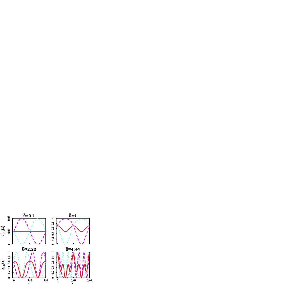
FIG. 2.: Population gratings in the $G^{\prime}$ manifold for several values of $\bar{\theta}.$ The three curves in each graph correspond to different initial conditions. Solid line: $\rho_{G,\frac{1}{2};G\frac{1}{2}}=\rho_{G,-\frac{1}{2};G-\frac{1}{2}}=1/2,$ dashed line: $\rho_{G,\frac{1}{2};G\frac{1}{2}}=1,$ dot-dashed line: $\rho_{G,-\frac{1}{2};G-\frac{1}{2}}=1,$.

In the far detuned case, max$\left\{\left|\delta\right|,\text{ }\left|A_{GG}^{\left(\alpha j,\alpha j\right)}\right|,\text{ }\left|A_{G^{\prime}G^{\prime}}^{\left(\alpha j,\alpha j\right)}\right|\right\}\gg\tau^{-1},$ instantaneous diagonalization of Eqs. (72) for the $\left|G=1/2,1/2\right\rangle$ and $\left|G^{\prime}=1/2,1/2\right\rangle$ states leads to spatially periodic potentials

$$U_{1,2} = 2^{-1}3^{-1/2}\hbar\left\{-A_{GG}^{\left(\alpha j,\alpha j\right)}\left(0\right)-A_{G^{\prime}G^{\prime}}^{\left(\alpha j,\alpha j\right)}\left(0\right)\pm\left[\left(3^{1/2}\delta+\left(A_{G^{\prime}G^{\prime}}^{\left(\alpha j,\alpha j\right)}\left(0\right)-A_{GG}^{\left(\alpha j,\alpha j\right)}\left(0\right)\right)\right)^{2}\right.\right.$$ (89)

$$+\left.\left.2\left(A_{G^{\prime}G}^{\left(11,21\right)}\left(1\right)\right)^{2}+4\left(A_{G^{\prime}G}^{\left(21,22\right)}\left(0\right)\right)^{2}+2^{5/2}A_{G^{\prime}G}^{\left(11,21\right)}\left(1\right)A_{G^{\prime}G}^{\left(21,22\right)}\left(0\right)\sin\left(4kz\right)\right]^{1/2}\right\}.$$

Potentials for the $\left|G=1/2,-1/2\right\rangle\$and $\left|G^{\prime}=1/2,-1/2\right\rangle$ states are shifted from these by $\lambda/8.$ For $\delta>3^{-1/2}\left(A_{GG}^{\left(\alpha j,\alpha j\right)}\left(0\right)-A_{G^{\prime}G^{\prime}}^{\left(\alpha j,\alpha j\right)}\left(0\right)\right),$ the potentials $U_{1}$ are responsible for phase changes of the initial state amplitudes. In the free evolution following the atom-field interaction, these atom phase gratings would be converted into amplitude gratings and the populations at the potential minima would focus at some specific time following the interaction. Atoms in the $m_{g}=+\frac{1}{2}$ Zeeman sublevel focus at $z=3\pi/8k,$ $7\pi/8k$ $\ldots$, while those in the $m_{g}=-\frac{1}{2}$ focus at $z=\pi/8k,$ $5\pi/8k$ $\ldots$ If both sublevels are equally populated then one obtains a $\lambda/8$-period grating of focused atoms that is the analogue of the $\frac{\lambda}{4}$-period gratings observed using a single photon transition in Cr atoms [14].

IV Multicolor fields

In analogy with the multicolor field geometry for single photon transitions [9], it is possible to suppress low order harmonics in the Raman scheme by using a geometry involving the three pairs of counterpropagating fields ${\bf F}=\left\{{\bf E,E}^{\prime}\right\},$ ${\bf F}_{1}=\left\{{\bf E}_{1}{\bf,E}_{1}^{\prime}\right\}$ and ${\bf F}_{2}=\left\{{\bf E}_{2}{\bf,E}_{1}^{\prime}\right\}$ shown in Fig. 3, connecting an initial ground state level $G$ to a final ground state level $G^{\prime}$ via an excited state $H.$ It is assumed that $\left|\Omega_{1}-\Omega\right|\tau\gg 1.$ Field ${\bf F}$ has effective propagation vector 2k, while fields ${\bf F}_{1}$ and ${\bf F}_{2}$ have effective propagation vector $-2{\bf k}$.

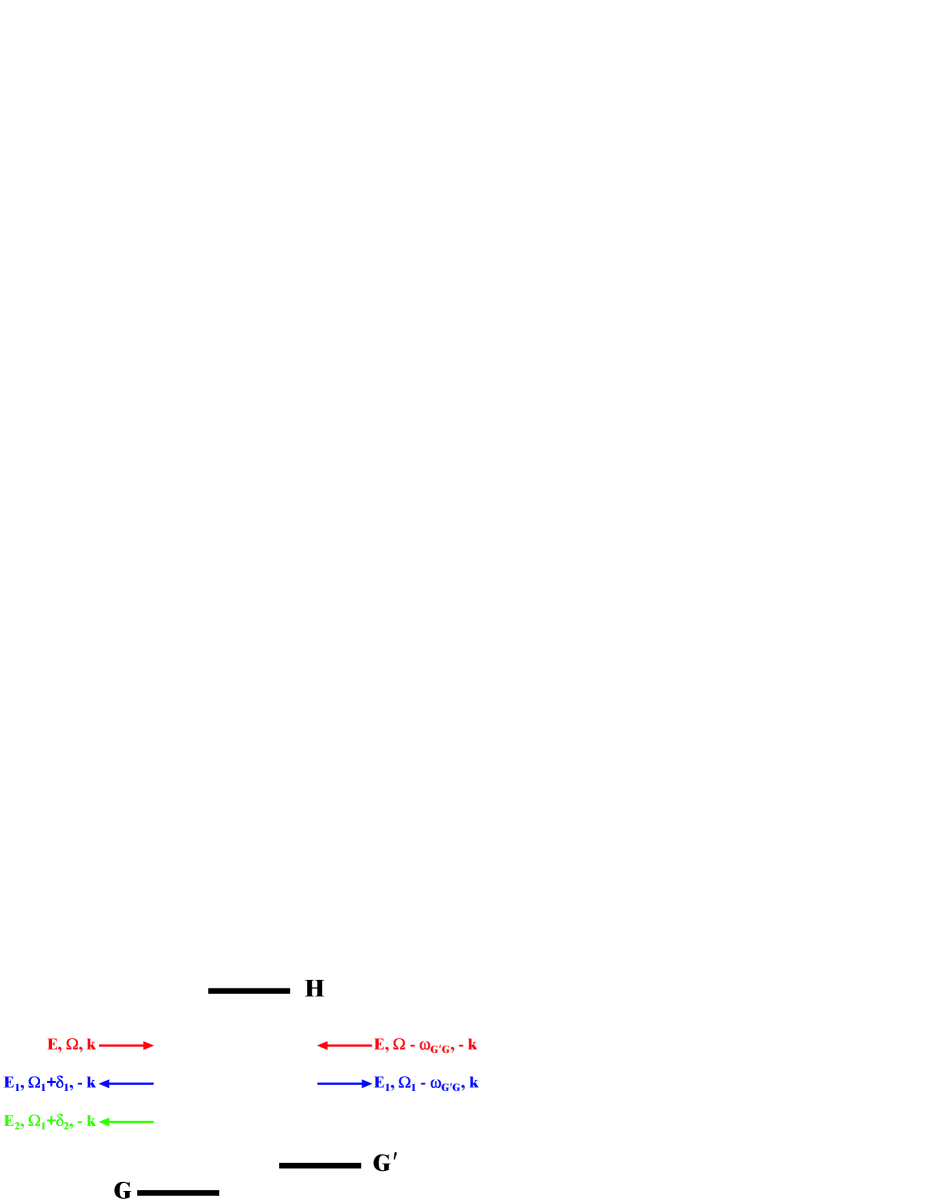
FIG. 3.: Multicolor Raman configuration

When the Raman detunings are large, $\left|\delta_{j}\right|\tau\gg 1,$ basic Raman processes are suppressed; however, by choosing $n_{1}\delta_{1}+n_{2}\delta_{2}=0$, where $n_{1}$ and $n_{2}$ are positive integers, one can produce nearly sinusoidal, high-order gratings. For example, if $\delta_{1}=-\delta_{2}$ and $\delta=0,$ to lowest order in the atom field coupling, there are two resonant contributions to the $G\rightarrow G^{\prime}$ transition amplitude, shown schematically in Fig. 4. One contribution is associated with a two-quantum process and varies as $\exp\left(2ikz\right)$ while the other is associated with a six-quantum process and varies as $\exp\left(-6ikz\right).$ In contributing to the final state probability, these terms interfere and result in a $\frac{\lambda}{8}$-period population grating. For arbitrary $n_{1}$ and $n_{2}$ one produces a $\frac{\lambda}{4\left(n_{1}+n_{2}\right)}$-period grating. By choosing $\left|\delta\right|\tau\gg 1$, one can produce high-order phase gratings. The higher order gratings can simultaneously have near unity contrast and nearly sinusoidal shape[9]. This is an important advantage of the multicolor field technique over the basic Raman configuration if one wishes to produce nearly sinusoidal, high-order, high contrast atom gratings.

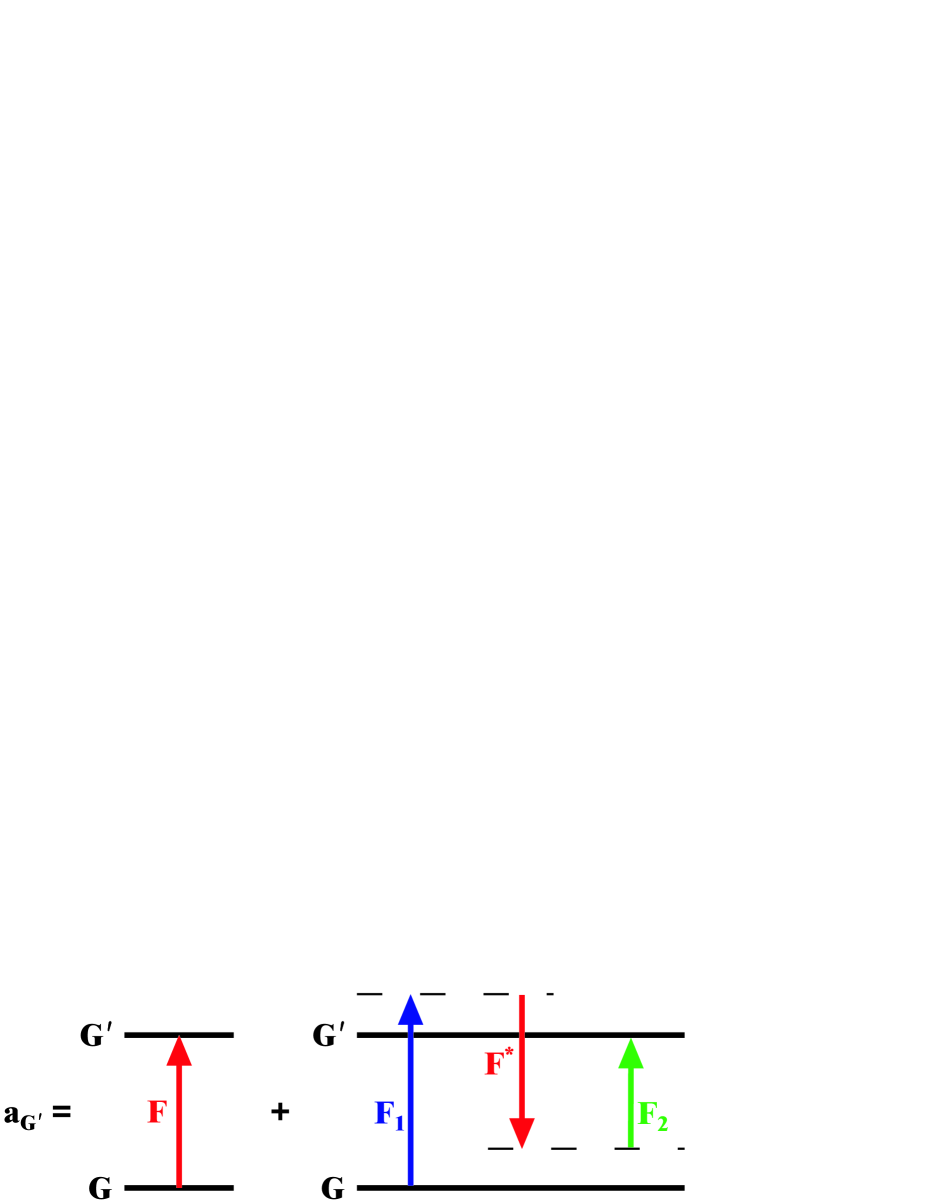
FIG. 4.: Contributions to $G\rightarrow G^{\prime}$ transition amplitude when $\delta_{1}=-\delta_{2}.$

The resulting equations are completely analogous to those obtained previously for the case of single-photon transitions [9] and will not be repeated here. There are two important differences between the two cases, aside from the fact that single-photon Rabi frequencies are replaced by two-photon Rabi frequencies. In order to satisfy the adiabaticity requirements necessary to suppress the lower harmonics, it is essential that the detunings $\left|\delta_{j}\right|$ be larger than any relevant characteristic frequencies in the problem such as decay rates or relative light shifts. In the case of single-photon transitions this led one to choose the field intensities such that $\chi_{\alpha}^{2}/\Delta_{1}+\chi_{\beta}^{2}/\Delta_{2}=0$, where $\chi_{\alpha},\chi_{\beta},\Delta_{1},\Delta_{2}$ are single photon Rabi frequencies and detunings, and to limit the pulse durations to values for which $\gamma_{e}\tau\ll 1,$ where $\gamma_{e}$ is an excited state decay rate [9]. The limitation placed on the pulse duration necessitates the use of stronger fields to reach higher order harmonics [9]. In the case of ground state transitions, there is no longer any significant restriction on pulse duration since the initial and final states are long-lived. However, the requirements on the relative light shifts remains the same with the replacement of single photon Rabi frequencies and detunings by the corresponding two-photon Rabi frequencies and detunings; moreover, the single photon detunings $\Delta_{H,G}^{\left(j\right)}$ should be chosen to cancel the first-order relative light shifts.

It is also possible to use an alternative approach to produce higher order gratings. Cataliotti et al. [15] detuned their Raman fields such that $\delta=\omega_{G^{\prime}G}/n$, where $n$ is a positive integer, and observed transitions for $n$ as large as 25. In other words, they monitored a multiphoton Raman transition, requiring $n$ Raman fields to achieve resonance. They used copropagating fields, but if the copropagating fields are replaced by counterpropagating fields, the multiphoton Raman field acts as a traveling wave field having propagation vector $2n{\bf k}$. If a second Raman field having a different carrier frequency and an effective propagation vector -$2n{\bf k}$ is added, one creates a ”standing wave” multiphoton Raman field varying as $\cos(2n{\bf k\cdot r)}$. In this manner one can create atom gratings having periodicity $\lambda/4n$.

V Discussion

It has been shown that it is possible to use optical fields having wavelength $\lambda$ to create atom amplitude and phase gratings having period $\lambda/4$ and $\lambda/8$ using a basic Raman geometry, or $\lambda/4(n_{1}+n_{2})$ using a multicolor field geometry. Once the gratings are created, the question remains as how to image the gratings at some distance $L$ from the atom-field interaction zone. This question has been addressed in detail in a previous publication [9] for both amplitude and phase gratings. For highly collimated beams, the phase gratings evolve into a focused array of lines having spacing $\lambda/4(n_{1}+n_{2})$ which could be deposited on a substrate. For atom beams having a higher angular divergence, echo techniques can be used to generate gratings with even smaller periodicities at specific focal planes [9]. As such, the basic and multicolor Raman geometries offer interesting possibilities for atom nanofabrication.

It is interesting to return to Eqs. (28) for cw fields. As mentioned earlier, the eigenvalues of the Hamiltonian correspond to the optical potentials for the ground state manifold. Since these optical potentials have period $\lambda/4$ or smaller, the normal or multicolor Raman field geometry can be used to produce optical lattices having this reduced periodicity. As an illustrative example, we consider the level scheme of Sec. III D involving two ground state manifolds with $G=1/2$ and $G^{\prime}=1/2$ that are connected to an excited state by four fields in the basic Raman geometry; {$E_{11},$ $\Omega_{11}=\Omega_{1},$ ${\bf k}_{11}={\bf k,}$ ${\bf e}_{11}={\bf\hat{x}\}}$, {$E_{21},$ $\Omega_{21}=\Omega_{1}-\omega_{G^{\prime}G}-\delta,$ ${\bf k}_{21}=-{\bf k,}$ ${\bf e}_{21}={\bf\hat{y}\}}$, {$E_{12},$ $\Omega_{12}=\Omega_{2},$ ${\bf k}_{12}=-{\bf k,e}_{12}={\bf\hat{x}\}}$, {$E_{2},$ $\Omega_{22}=\Omega_{2}-\omega_{G^{\prime}G}-\delta,$ ${\bf k}_{22}={\bf k,}$ ${\bf e}_{22}={\bf\hat{x}\}}.$ The corresponding optical potentials produced are given by Eq. (89). If atoms are prepared in the $G$ manifold and $\delta$ is sufficiently large to enable one to adiabatically eliminate the $G^{\prime}$ state amplitudes, one finds that the ground state amplitudes in the $G$ manifold evolve as

$$a_{G,\pm\frac{1}{2}} \propto \exp\left(-iU_{\pm}t/\hbar\right)a_{G,\pm\frac{1}{2}}^{-},$$

$$U_{\pm} = \pm 2^{1/2}\hbar\left(A_{G^{\prime}G}^{\left(11,21\right)}\left(1\right)A_{G^{\prime}G}^{\left(12,22\right)}\left(0\right)/3\delta\right)\sin\left(4kz\right)$$

In other words, the $m_{g}=1/2$ sublevel is subjected to the $U_{+}$ potential and the $m_{g}=-1/2$ sublevel is subjected to the $U_{-}$ potential. If cold atoms are trapped in these potentials the atomic density will have $\lambda/8$ periodicity. Even smaller periodicities are possible using a multicolor geometry. Calculations of the optical potentials for more complicated level schemes and field geometries, such as those appropriate to the alkali metal atoms, are deferred to a future planned publication.

VI Acknowledgments

The extension of our previous work on multicolor geometries to the Raman case was suggested to us by Tycho Sleator at New York University. We are pleased to acknowledge helpful discussions with G. Raithel at the University of Michigan. This work is supported by the U. S. Office of Army Research under Grant No. DAAD19-00-1-0412 and the National Science Foundation under Grant No. PHY-9800981, Grant No. PHY-0098016, and the FOCUS Center Grant, and by the Office of the Vice President for Research and the College of Literature Science and the Arts of the University of Michigan.

REFERENCES

- [1] For a recent review, see P. R. Berman and D. G. Steel, ”Coherent Optical Transients,” in Handbook of Optics, Vol. IV, edited by M. Bass, J. Enoch, E. van Stryland, and W. Wolfe (McGraw-Hill, New York, 2001) chap. 24.
- [2] N. A. Kurnit, I. D. Abella, and S. R. Hartmann, Phys. Rev. Lett. 13, 567 (1964).
- [3] R. Kachru, T. J. Chen, S. R. Hartmann,T. W. Mossberg, and P. R. Berman, Phys. Rev. Lett. 47, 902 (1981).
- [4] R. Beach, S. R. Hartmann, and R. Friedberg, Phys. Rev. A 25, 2658 (1982); R. Friedberg and S. R. Hartmann, Phys. Rev. A 48, 1446 (1993); R. Friedberg and S. R. Hartmann, Laser Phys. 3, 1128 (1993).
- [5] C. J. Bordé, Phys. Lett. A 140, 10 (1989: R. Friedberg and S. R. Hartmann, Laser Phys. 5, 526 (1993); for a review of atom interferometry, see Atom Interferometry, edited by P. R. Berman (Academic Press, San Diego, 1997).
- [6] R. G. Brewer and R. L. Shoemaker, Phys. Rev. A 6, 2001 (1972).
- [7] T. Mossberg, A. Flusberg, R. Kachru, and S. R. Hartmann, Phys. Rev. Lett. 39, 1523 (1977); 42, 1665 (1979).
- [8] B. Dubetsky and P. R. Berman, Phys. Rev. A 50, 4057 (1994).
- [9] P. R. Berman, B. Dubetsky, and J. L. Cohen, Phys. Rev. A 58, 4801 (1998).
- [10] For the analogue with single photon transitions to be correct, it is necessary that the Raman fields obey a directionality property that is discussed at the beginning of Sec. III A.
- [11] P. R. Berman, Phys. Rev. A 53, 2627 (1996).
- [12] There are only a few atoms which have hyperfine sublevels belonging to different fine structure manifolds. One such atom is Sm, for which the Raman transition can be driven by optical radiation at nm and nm.
- [13] J. L. Cohen, B. Dubetsky, and P. R. Berman, Phys. Rev. A 60, 3982 (1999).
- [14] R. Gupta, J. J. McClelland, P. Marte, R. J. Celotta, Phys. Rev. Lett. 76, 4689 (1996).
- [15] F. S. Cataliotti, R. Scheunemann, T. W. Hänsch, and M. Weitz, Phys. Rev. Lett. 87, 113601 (2001).