Simulations of binary hard-sphere crystal-melt interfaces: interface between a one-component fcc crystal and a binary fluid mixture

Abstract

The crystal-melt interfaces of a binary hard-sphere fluid mixture in coexistence with a single-component hard-sphere crystal is investigated using molecular-dynamics simulation. In the system under study, the fluid phase consists of a two-component mixture of hard spheres of differing size, with a size ratio $\alpha=0.414$. At low pressures this fluid coexists with a pure fcc crystal of the larger particles in which the small particles are immiscible. For two interfacial orientations, [100] and [111], the structure and dynamics within the interfacial region is studied and compared with previous simulations on single component hard-sphere interfaces. Among a variety of novel properties, it is observed that as the interface is traversed from fluid to crystal the diffusion constant of the larger particle vanishes before that of the small particle defining a region of the interface where the large particles are frozen in their crystal lattice, but the small particles exhibit significant mobility. This behavior was not seen in previous binary hard-sphere interface simulations with less asymmetric diameters.

I Introduction

A fundamental understanding of the nucleation, growth kinetics and morphology of crystals grown from the melt requires a detailed microscopic description of the crystal-melt interfaceWoodruff (1973); Tiller (1991); Howe (1997); Adamson and Gast (1997). However, such interfaces are very difficult to probe experimentally and reliable experimental data, especially for structure and transport properties, is rare. It is then not surprising that computer simulations have, in recent years, played a leading role in the determination of the microscopic structure, dynamics and thermodynamics of such systemsLaird (1998).

To date, the vast majority of simulation studies have focused on single component interfacial systems. Such studies range from simple model systems such as hard spheresKyrlidis and Brown (1995); Mori et al. (1995); Laird (1998); Davidchack and Laird (2000) or Lennard-JonesBroughton and Gilmer (1986); Galejs et al. (1989) to more “realistic” systems, such as waterKarim and Haymet (1988); Karim et al. (1990); Hayward and Haymet (2001), siliconAbraham and Broughton (1986); Landman et al. (1986) or simple metalsJesson and Madden (2001); Hoyt et al. (2001). In contrast, there have been but few studies on multicomponent systemsDavidchack and Laird (1996, 1999), in spite of the fact that most materials of technological interest are mixtures (for example, doped semiconductors, alloys and intermetallic compounds). In such systems, the crystal and coexisting fluid have differing composition, in general, and the change in concentration as one traverses the interface from one bulk phase into the other becomes an object of study.

Of particular interest to materials scientists is the degree of interfacial segregation - the preferential adsorption of one component (usually the “solute”) at the interface. In addition, the phase diagrams for multi-component systems are significantly more varied and complex than single component systems due to the additional dimension of concentration. For a binary system several types of solid-liquid equilibria are possible. If the two types of particles are similar, then one typically has coexistence between a binary fluid and a substitutionaly disordered solid of similar structure to that of the pure components. However, if the two types of particles are substantially different in nature, then generally the binary fluid will either be immiscible in the pure coexisting solid, or will coexist with one or more ordered crystal mixtures (e.g. intermetallic compounds). Previous simulation studies on binary crystal-melt interfaces have exclusively focused on the former case, namely the equilibrium between the fluid and a disordered crystal. Davidchack and LairdDavidchack and Laird (1999) recently reported results for a binary hard sphere system in which a substitutionally disordered face-centered-cubic (fcc) crystal coexists with a binary fluid mixture. In a related study, Hoyt et al. examined the crystal-melt interface of a Cu/Ni mixtureHoyt et al. (2001). In both studies the degree of solute segregation was found to be negligible.

In the two studies above, the disordered fcc crystal was stabilized by the fact that the two components were quite similar in size -for example, in the hard-sphere system studied by Davidchack and Laird, the diameters of the two types of spheres making up the system differed only by 10%. In this work, we extend the previous studies to hard-sphere mixtures with significant size asymmetry. For such systems, in which the diameters differ by more than about 85%, the disordered fcc phase is no longer stable and only coexistence of the fluid with ordered crystal structures is possible. In this work we examine the interface between a binary hard-sphere fluid mixture and a coexisting fcc crystal in which the small particle is immiscible.

Our system of choice is a binary hard-sphere mixture in which the ratio of the smaller particle diameter to that of the larger particle is 0.414. Hard spheres are an important reference system for the crystal-melt interfaces of simple systems since the structure, dynamics and phase behavior of dense atomic systems are dominated by packing considerations with only minor influence from the attractive parts of the interactions. For example, it has been recently demonstratedLaird (2001) that the interfacial free energy of close-packed metals can be quantitatively described using a purely hard sphere model. The specific diameter ratio of 0.414 was chosen because, to perform an interface simulation, accurate phase coexistence parameters are required a priori, and the phase diagram for this binary system has been worked out via simulation in some detailTrizac et al. (1997). This phase diagram shows that at low pressures the fluid mixture coexists with a pure fcc crystal of the larger particles, but that at higher pressures the crystal structure in equilibrium with the fluid is a 1:1 (or AB) “intermetallic” compound with an “NaCl” structure (the small and large particles form interpenetrating fcc lattices). (The existence of the “NaCl” structure at this diameter ratio had been predicted earlier, using cell theoryCottin and Monson (1995). The diameter ratio, $\alpha=0.414$ is necessary for an “NaCl” structure to attain its maximum packing fraction of 0.793.) Thus, this system allows us to study the interfaces between binary fluids and two types of ordered crystal phases: single component and “NaCl”. In this work we present results for the former, but simulations on the fluid/“NaCl” are under way and will be reported later.

II Description of the System

We consider a two-component system consisting of hard spheres of differing diameters, given by $\sigma_{A}$ and $\sigma_{B}$. Without loss of generality, it is assumed that $\sigma_{A}\geq\sigma_{B}$. The interaction between two particles of type $i$ and $j$, ($i,j\in\{A,B\}$), respectively, is then given by

$$\phi_{ij}(r)=\left\{\begin{array}[]{r@{\quad,\quad}l}\infty&r\leq\sigma_{ij}\\ 0&r>\sigma_{ij}\end{array}\right.,$$ (1)

where $r$ is the distance between the centers of the two interacting spheres, and $\sigma_{ij}$ is the distance of closest possible approach. In addition, we define the spheres to be additive, that is, $\sigma_{ij}=(\sigma_{i}+\sigma_{j})/2$. The state of the system is then completely described by specifying the total density, $\rho=\rho_{A}+\rho_{B}=N/V$, the mole fraction, $x_{A}$, of the larger species, and the diameter ratio $\alpha=\sigma_{B}/\sigma_{A}$. Note that so defined one has $\alpha\in(0,1)$. In a single component system composed of hard spheres of diameter $\sigma$ the packing fraction, $\eta$ (the fraction of the total volume occupied by the spheres) is given by,

$$\eta=\frac{\pi}{6}\rho\sigma^{3},$$ (2)

where $\rho$ is bulk density. For the binary hard sphere system described above the packing fraction is

$$\eta = \eta_{A}+\eta_{B}$$ (3)

$$= \frac{\pi}{6}\rho\left[x_{A}\sigma_{A}^{3}+x_{B}\sigma_{B}^{3}\right]$$ (4)

$$= \frac{\pi\sigma_{A}^{3}}{6}\rho[x_{A}+(1-x_{A})\alpha^{3}]\;.$$ (5)

As mentioned in the introduction we are interested in the present study in the interface between an fcc crystal consisting of pure large (type A) spheres and its coexisting binary fluid at a diameter ratio, $\alpha=0.414$. The pressure-composition phase diagram for a binary hard sphere system with this diameter ratio has been previously determined by Trizac and coworkersTrizac et al. (1997) and is shown in Fig. 1.

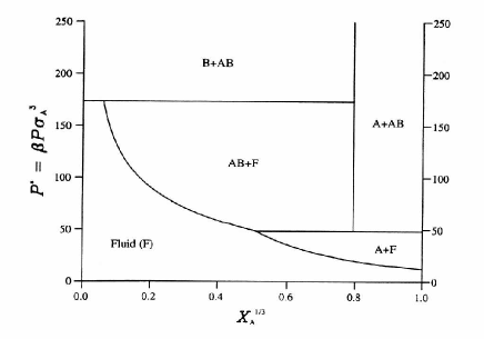
Figure 1: Pressure-concentration phase diagram of a binary hard-sphere system with $\alpha=0.414$. [Reprinted from Ref. 22, by permission of the publisher, Taylor and Francis Ltd. (www.tandf.co.uk/journals).] Note that to make the phase coexistence lines easier to distinguish, the pressure is plotted against $x_{A}^{1/3}$ and not $x_{A}$ as in the usual case.

For this study we have chosen the point in the phase diagram where a fluid mixture with a 1:1 composition (that is, $x_{A}=0.50$) coexists with a crystal phase that is an fcc composed of only large particles. We independently calculated the coexistence conditions for this point in the phase diagram and we determine the coexisting pressure to be $P=20.1\sigma_{A}^{3}/kT$, with packing fractions for the crystal and fluid calculated to be $\eta_{c}=0.61$ and $\eta_{f}=0.51$, respectively.

III Calculation of Interfacial Profiles

To monitor changes in the structural or dynamical properties across the interface, the system is divided into bins along the $z$-axis, defined as that perpendicular to the interfacial plane. Quantities of interest are then calculated for each bin generating a $z$-dependent interfacial profile for the specific property (density, concentration, diffusion, etc.) being measured. The techniques of profile generation and analysis are similar to those used earlier in the works of Davidchack and Laird on the singleDavidchack and Laird (1998) and binary hard-sphere systems (with $\alpha=0.9$)Davidchack and Laird (1999). In this section these techniques are summarized, with particular attention to the present calculation. The reader is urged to consult the earlier papers if more detail is required.

In our analysis of the simulations, we employ bins of two different resolutions: a coarse scale and a fine scale. Coarse scale bins have a width equal to the layer spacing of the bulk crystal. This spacing is $0.753\sigma_{A}$ for [100] and $0.870\sigma_{A}$ for [111]. The fine scale is $1/25$ of the coarse scale. Fine scale bins reveal in greater detail parameter variations across the interface, but the coarse scale is more useful for observing overall trends in the interfacial profiles. Also for some parameters, such as the diffusion constant, only the coarse scale can be used if one is to achieve meaningful statistical accuracy. For interfacial profiles that exhibit oscillations on the order of the lattice spacing, such as density, the conversion between the fine-scale profiles and coarse-scale profiles to illustrate bulk trends is problematic, since the distance between the peaks of such profiles is not necessarily constant through the interface. The mismatch between the coarse-scale bins and the peak spacing can lead to spurious resultsDavidchack and Laird (1998) if one simply averages over the fine scaled bins to create the coarse scaled profile. For such profiles we employ a Finite Impulse Response filtering procedurePress et al. (1992) to average out the oscillations and reveal coarse-grained trends. Details of the specific filtering procedure we use can be found in Ref. 24.

Below is a description on how the various interfacial properties were determined. In the definitions, the size of the bin is denoted by $\Delta z$ and $L_{x}$, $L_{y}$ and $L_{z}$ are the the dimensions of the simulation box in the $x$, $y$ and $z$ directions, respectively.

• Pressure: The total pressure profile is defined as

  $$P(z)=\frac{1}{3}\left\{P_{xx}(z)+P_{yy}(z)+P_{zz}(z)\right\}\;,$$ (6)

  where$P_{kk}$ is calculated from

  $$\frac{P_{kk}}{k_{B}T}=\rho(z)+\frac{3m}{2L_{x}L_{y}\Delta z\Delta t\!\!<E_{k}>\!\!}\sum_{c=1}^{N_{c}}r^{(c)}_{k}\Delta v^{(c)}_{k},$$ (7)

  where $c$ indexes the collisions, $m$ is the mass of each sphere, $\!\!<E_{k}>\!\!$ is the average kinetic energy per sphere, $N_{c}$ is the number of collisions that occurred over the time interval $\Delta t$ in the region between $z-\Delta z$ and $z+\Delta z$, $r^{(c)}_{k}$ is the $kth$ component of the relative distance between the two colliding spheres and $\Delta v^{(c)}_{k}$ is the $kth$ component of the change in velocity for collision $c$. The first term in Eq. 7 represents the ideal gas pressure and the second term is the excess part due to sphere interactions.

• Excess Stress Profiles: The local excess stress is calculated from the pressure tensor components.

  $$S(z)=P_{zz}(z)-\frac{1}{2}\{P_{xx}(z)+P_{yy}(z)\}$$ (8)

  In a simulation of an equilibrium interfacial system this quantity should be zero, except in a small region at the interface. Improper preparation or equilibration of the system often manifests itself in the excess of this quantity in the bulk crystal away from the interface. As such this quantity is carefully monitored as a measure of the quality of the simulation. To smooth out the large oscillations in this quantity through the interface, the profile is filtered to easily reveal overall trends. (The local excess stress can be integrated with respect to $z$ to give the surface excess stress. For a liquid-vapor interface the surface excess stress is identical to the interfacial free energy, but since the relaxation time for stress in a crystal is generally much longer than a typical simulation time, the surface excess stress and $\gamma_{sl}$ can be significantly different for crystal-melt interfacesTiller (1991).)

• Density Profiles and Contour Plots: The fine-scale density profile for a sphere of type $i$ is determined from the number density of that type particle in each fine-scale bin.

  $$\rho_{i}(z)=\frac{<\!\!N_{i}(z)\!\!>}{L_{x}L_{y}\Delta z}$$ (9)

  where $<\!\!N_{i}(z)\!\!>$ is the average number of spheres of type $i$ in the region between $z-\Delta z/2$ and $z+\Delta z/2$. To observe overall trends in bulk density (or concentration) changes we also produce filtered density profiles using our FIR filtering procedure discussed above.

  In addition to the $z$ dependent density profiles, it is also useful to examine the density variations within the x-y planes parallel to the interfacial plane. To do this we divide the system into orthorhombic subcells with a width in the $z$ direction equal to the coarse bin spacing and $x$ and $y$ dimensions of $0.15\sigma_{A}$. By counting the average number of particles of each type in each subcell and dividing by the subcell volume we can produce 2d contour plots of the cross-sectional density variation within each interfacial plane.

• Interface location: We determined the location of the interface from the orientational order parameter profile.

  $$q_{n}(z)=\left<\frac{1}{N_{z}}\sum_{i,j,k}cos\left\{n\theta_{xy}(i,j,k)\right\}\right>$$ (10)

  where $n$ is an integer, $i,j$ and $k$ are nearest neighbor atoms, $\theta_{xy}(i,j,k)$ is the bond angle formed by $i,j$ and $k$ projected on the $x,y$ plane, and $N_{z}$ is the total number of atoms that form bond angles. The average is taken over the number of angles found between $z-\Delta z/2$ and $z+\Delta z/2$. The interface in the [100] orientation is the point along the $z$-axis where $q_{4}$($q_{6}$ for the [111]) is the arithmetic mean of the bulk crystal and liquid values. For comparison, the position of the Gibbs dividing surfaceTiller (1991) is also calculated. We determine the Gibbs dividing surface as the plane along the z-axis such that for the ’solute’ $i$, $\Gamma^{i}=0$ in the equation

  $$N^{i}/A=\rho_{S}^{i}z+\rho_{L}^{i}(L_{z}-z)+\Gamma^{i}$$ (11)

  where $N^{i}$ the total number of spheres of type $i$, $A$ is the area of the interface, $\rho_{S}^{i}$ and $\rho_{L}^{i}$ are the bulk densities, $z$ is the location of the interface assuming the length of the simulation box runs from $0$ to $L_{z}$ and $\Gamma^{i}$ is the excess particle per unit area of the interface.

• Diffusion coefficient profile: To study the dynamics across the interface, the diffusion coefficient profile is calculated. For a particle of type $i$, the diffusion coefficient is defined as follows

  $$D_{i}(z)=\frac{1}{6N_{i}(z)}\frac{d}{dt}\sum_{j=1}^{N_{i}(z)}\left<{\mbox{\boldmath$r$}_{j}(t)-\mbox{\boldmath$r$}_{j}(t_{0})}^{2}\right>$$ (12)

  The term in the summation is the mean squared displacement over a time interval $t-t_{0}$ of a total of $N_{i}$ type $i$ spheres located between $z-\Delta z/2$ and $z+\Delta z/2$ at time $t_{0}$.

IV Construction and Equilibration of Interface

Initially, blocks of crystal and fluid spheres at the calculated coexistence packing fractions and concentrations were prepared separately. As a reference, the $z$-axis is taken to be perpendicular to the interface. The x-y planes for both blocks had the same dimensions so that they would fit perfectly when put together to construct the interface. The plane perpendicular to the interface is made as close to square as possible given the geometric constraints of the specific interfacial orientation under study. This is trivial to achieve with the [100] orientation but for [111], the $x$ and $y$ lengths can only be made approximately equal. The lengths along $z$ were made longer than both those in $x$ and $y$ so that bulk properties will be observed between the two interfaces formed. Periodic boundary conditions are applied in all directions, which results in the two independent crystal-melt interfaces formed along $z$. The similarity of the two interfaces is an important monitor on the quality of the simulation. Obviously, if statistically significant differences in structure or dynamics exist between the two interfaces, then the system has not been properly equilibrated.

The crystal block with [100] orientation was set up with 7776 large spheres. It consisted of 48 crystal layers, each layer having 162 spheres. Using the coexistence packing fraction $\eta_{c}=0.61$, the following dimensions for the [100] crystal block were used: $L_{x}=13.56\sigma_{A}$, $L_{y}=13.56\sigma_{A}$ and $L_{z}=36.15\sigma_{A}$. Its coexisting fluid had 7776 large spheres and 7776 small spheres (15552 spheres total). The block length is $L_{z}=43.78\sigma_{A}$. For reasons that will be explained later, this $L_{z}$ gives a packing fraction that is slightly higher than that obtained from the calculated coexistence conditions. For the simulation of the [111] interface, the crystal block used contained 8190 large spheres, with 45 layers in the $z$ direction giving 182 spheres per layer. The crystal block dimensions are $L_{x}=13.85\sigma_{A}$, $L_{y}=12.91\sigma_{A}$ and $L_{z}=39.13\sigma_{A}$. The total number of fluid spheres used was also 15552 as in that for the [100] simulation with $L_{z}=45.09\sigma_{A}$, again, giving a packing fraction slightly higher than that predicted for coexistence. Thus the total number of particles in the interface simulations are 23328 and 23742 for the [100] and [111] interfacial orientations, respectively.

Both crystal and fluid blocks are equilibrated separately. The two blocks are then put together but a gap equal to $\sigma_{A}$ is left between each of the two crystal-melt interfaces formed to ensure that no initial overlap will occur at the interfaces. The molecular dynamics simulation is then started with only the fluid spheres allowed to move (the crystal spheres remain fixed). The fluid then fills the gaps. To compensate for the decrease in the overall bulk density of the fluid phase during this step, the fluid blocks are prepared at a packing fraction that is slightly higher than the predicted coexistence values (as mentioned earlier). In the next step, the crystal is equilibrated with the fluid spheres held fixed. At this point the interface setup is complete and an equilibration run is started with all spheres moving and with initial velocities assigned according to a Maxwell distribution. In order to efficiently carry out the molecular dynamics simulation of such a large system we use the cell method of Rappaport Rappaport (1995).

The stability of a crystal-melt interface in a simulation is extremely sensitive to the assumed coexistence conditions. In our previous workDavidchack and Laird (1998, 1999), it was found that the predetermined coexistence conditions generally had to be modified slightly in order to create a stationary interface with a zero excess stress in the bulk crystal region. This is necessary because a) the coexistence conditions are often not known a priori to the accuracy required for interface stability and b) the presence of the interface in a finite simulation can shift the coexistence equilibrium slightly. During our preliminary runs for the current system, using the coexistence conditions as calculated by thermodynamic integration of the free energies of separate bulk phases, we found that the resulting interface was stable, but yielded a bulk crystal with negative excess stress. Through experimentation, we found that an equilibrium interface with zero crystal excess stress was possible if the initial fluid packing fraction was increased to $\eta_{f}=0.52$. This had the effect of changing the concentration equilibrium slightly away from a 1:1 mixture in the fluid, as discussed below. Now it is in principle possible to vary both the initial fluid concentration and packing fraction so that the final equilibrium gives precisely a 1:1 fluid mixture, however this procedure is quite tedious and since our choice of the 1:1 fluid at coexistence was arbitrary, the fact that the actual system deviates slightly from this concentration is not important for the purposes of the current study.

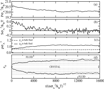
Figure 2: Time evolution of (a) total pressure of the system, (b) stress in bulk crystal, (c) fluid densities and (d) location of the interfaces, $z_{0}$. The time unit $(m\sigma_{A}^{2}/k_{B}T)^{1/2}$ corresponds roughly to 18 collisions per particle (cpp).

To ensure that the system is indeed in equilibrium and that the bulk crystal is free of excess stress, we monitor a variety of properties such as total pressure, bulk crystal stress, fluid bulk densities and interfacial location. The results for the [100] interface are shown in Fig. 2, which shows that prior to equilibration at about $t^{*}\equiv t(kT/m\sigma_{A}^{2})^{1/2}=10000$ the crystal grows by about 3 crystal lattice planes (see Fig. 2d), accompanied by a pressure drop from 20.6 to its equilibrium value of 20.1 $\sigma_{A}^{3}/k_{B}T$ (Fig. 2a). In addition, the average excess stress in the bulk crystal, initially positive, goes to zero (within flucuations) when equilibrium is reached (Fig. 2b). (This average excess stress was calculated by averaging $S$ as defined above over the middle 28 layers of the bulk crystal.)

Initially, the bulk densities of both particle types in the fluid are equal, but as the system equilibrates, the bulk density of the small particles increases. This increase is due to the growth of the crystal (see Fig. 2d). Large fluid particles near the crystal freeze, expelling the small particles, which are immiscible in the crystal at this pressure, into the bulk fluid region. Although the bulk fluid initially has a large sphere mole fraction of $X_{A}=0.50$, the value at equilibrium is somewhat lower (0.46 and 0.47 for the [100]and [111] interfaces, respectively). The equilibrium packing fraction of the bulk fluid slightly reduced from its initial value of $\eta_{f}=0.52$ to 0.51. Once the system is in equilibrium, the interfacial positions are stable and the fluctuation in position is less within one layer spacing.

In the preparation of the [100] interface some small particles became trapped within some of the interior crystal layers as the crystal grew during equilibration. Since these were in regions where the diffusion constant for the small (and large) particles was found to be zero, it cannot be determined whether these particles would actually be present in a true equilibrium interface. In order to determine the importance of these interstitial small particles in stabilizing the interface, we removed the particles (about 77 total) from the inner 3 crystal layers where they were found. The removal was done at $t^{*}=8000$ in the equilibration run. Initially the crystal stress became negative, but quickly returned to zero (within fluctuations) as small particles from the bulk diffused in to reoccupy the removed layer closest to the interface (this layer corresponds to layer B in Fig. 5, discussed in the next section). The inner two layers did not fill in. The interfacial position remained stable during this process. The question of true chemical equilibrium is always a tricky one in these types of interface simulationsDavidchack and Laird (1999) due to the extremely slow relaxation of concentration in the deeper crystal layers. However, in this region the concentration of small particles is in any event probably quite small and should not affect our results significantly (except for perhaps the interfacial segregation). As a possible check to this procedure, one could use the Widom insertion method Frenkel (1996) to determine the excess chemical potential, and thus the solubility, of the small particles in the various inner crystal layers, but this was not done here.

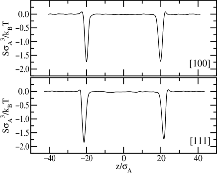
Figure 3: Filtered excess stress profiles for the [100] and [111] interface orientations.

The total length of the averaging run after equilibration was $t^{*}=4000$, which was divided into 40 separate blocks of length $t^{*}=100$ (corresponds to about 1800 collisions per particle(cpp)),over which the interfacial profiles were averaged. Since the system contains two interfaces, each block average yields two independent profiles (when properly folded about the center of the crystal) Thus, each of the profiles reported here represents an average of 80 block averages.

It is important to compare the two independent interfaces produced in a single interface simulation to ensure that they are statistically identical. Significant differences between the two interfaces are indications of problems with the equilibration procedure. As a diagnostic we determine the excess stress profile (calculated on the fine scale and filtered using the FIR filter described above and in Ref. 24). These filtered stress profiles are shown in Fig. 3 for both the [100] and [111] orientations - note that, the crystal is in the middle of the simulation box. The profiles are remarkably symmetric and also show that the excess stress is zero within fluctuations in the bulk crystal region. It should be noted that in contrast to the case for a liquid-vapor interface, the interfacial free energy of a crystal melt interface cannot be determined from the integral of the excess stress profile, as the relaxation time for stress in the crystal is significantly longer than possible simulation timesTiller (1991), and must be determined by other means, such as the recently developed cleaving wall methodDavidchack and Laird (2000). The excess stress profiles shown in Fig. 3 show a significant negative stress region on the crystal side of the interface, indicating that in this region the transverse pressure components are greater than the pressure component normal to the interfacial plane. The precise origin of this unrelaxed crystal stress at the interface is as yet unknown.

As mentioned above, the position of the interface is determined as the value of $z$ at which the orientational order parameter for the large spheres is the arithmetic mean of that quantity in the two bulk phases. This quantity is a useful measure of interfacial location as it is monotonic as a function of $z$ (so that using the arithmetic mean makes sense) and can be calculated as smooth function without large fluctuations using relatively short simulation runs. Orientational order parameters $q_{4}$ and $q_{6}$, as defined by Eqn. 10, were determined for each particle type. These are shown in Fig. 4. Since the crystal phase is made up of pure large spheres and we want to see how the ordering of particles is changed from bulk crystal to bulk liquid, we determined the interface location from the parameters calculated for large spheres. We also show $q_{4}$ and $q_{6}$ for the small particles and we see that at the interfacial region, the small spheres start developing some order that is similar to the large spheres.

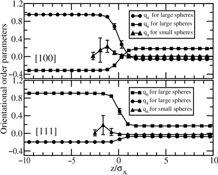
Figure 4: Orientational order parameters $q_{4}$ and $q_{6}$ for the two sphere types and for both interfaces studied.

V Results for the [100] and [111] Interfaces

V.1 Structure

The fine scale density profiles for the [100] and [111] interfaces are shown in the upper panels of Figures 5 and 6, respectively. Shown in the lower panels are the corresponding filtered profiles (including the total density profile). The distance along the $z$-axis (in units of the large particle diameter, $\sigma_{A}$) is measured relative to the interface center, defined as discussed above by the orientational order profiles. The vertical dotted lines are equally spaced and constructed to correspond with the density minima in between the bulk crystal layers. In both figures, specific interfacial layers are labeled alphabetically for later reference - layers A and G correspond to bulk crystal and liquid, respectively, and layers B-F lie within the interfacial region.

Figure 5: Fine-scale (upper panel) and filtered (lower panel) density profiles for the [100] orientation. The solid line and dashed lines are for the larger (A) and smaller (B) particles, respectively. In the lower panel the dotted line shows the filtered total density.

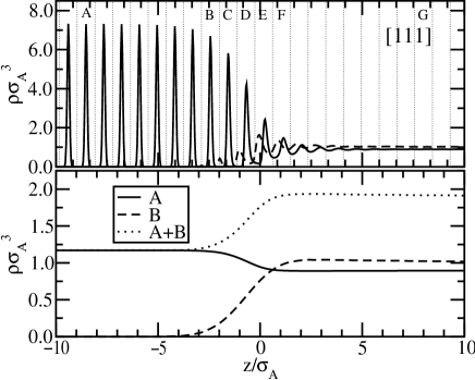
Figure 6: Fine-scale (upper panel) and filtered (lower panel) density profiles for the [111] orientation. The solid line and dashed lines are for the larger (A) and smaller (B) particles, respectively. In the lower panel the dotted line shows the filtered total density.

The density profiles for the large particles resemble strongly those for the single component hard sphere interfaceDavidchack and Laird (1998) with the periodic oscillations of the bulk crystal transforming to the uniform density of the fluid over about 7-9 lattice layers as the interface is traversed along the $z$-axis. The new feature seen in the present simulation is the decay of the small particle density over a similar distance into the bulk crystal, in which the small particle are immiscible. As the small particle density decreases into the crystal, it develops oscillations with a wavelength closely matching that of the crystal lattice spacing. For the [100] interface, the oscillations in the small particle density, $\rho_{B}(z)$ line up in phase with those of the large particle density,$\rho_{A}(z)$; whereas, in the [111] interface the oscillations are out of phase - the peaks of $\rho_{B}(z)$ correspond to minima of $\rho_{A}(z)$. Analysis of the atomic positions indicate that this difference is due to the fact that in the interfacial region the small particles occupy interstitial sites of the large particle fcc lattice - corresponding to the positions that would be occupied in an NaCl structure. These preferred positions lie in the [100] plane, but lie between the [111] planes of the bulk fcc lattice. Recall that the NaCl structure is the stable structure for this system at high pressure, so this effect is reminiscent of premelting transitions at solid/vapor interfaces below the bulk melting point, in that the presence of a nearby triple point (in this case the fcc/NaCl/fluid triple point) manifests itself in the presence of the metastable phase (NaCl) at the interface between the two coexisting phases (fcc and fluid).

As in the single component hard-sphere systemDavidchack and Laird (1998), the spacings between the density peaks exhibit some variation across the interface - especially for the [100] orientation. For each interface, the peak spacing was measured by determining the distance between density peaks in the fine scale profiles. The resulting peak spacings as functions of $z$ are shown in Fig. 7. For the large particles the dependence of the spacing on interfacial orientation and $z$ is identical to that seen in the single component simulationsDavidchack and Laird (1998). The spacing for the [100] lattice increases by nearly 20% from the bulk crystal value of 0.76$\sigma_{A}$ to the limiting value of about 0.9$\sigma_{A}$ as the bulk fluid is approached. The spacing for the large particles in the [111] interface has the same bulk liquid limiting value, but since the bulk crystal spacing is very close to this limiting value, the variation in spacing across the interface is quite small. The changes in peak spacing for the small particles are quite different for the different orientations and loosely follow those of the large particle - in [100] the small and large particle curves have very similar shape, but are shifted by about $\sigma_{A}$.

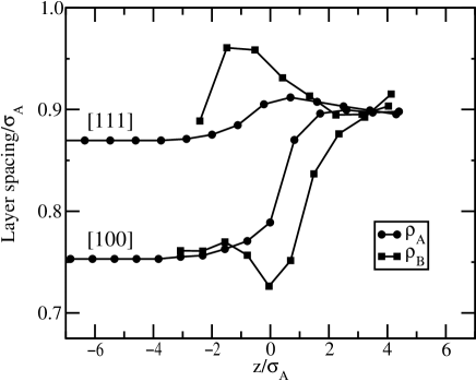
Figure 7: Peak spacing as determined from maxima of fine-scale density profiles for both interfaces studied.

It is useful to compare these results directly with the single component caseDavidchack and Laird (1998). In Fig. 8 we plot (upper panel) the fine scale density profiles for the [100] orientation of both the single component and binary interfaces. The single component data was shifted slightly along $z$ to make the liquid peaks commensurate. From this plot one sees that the presence of the small particles has negligble effect on the coexisting liquid density and structure; however, the higher pressure for the binary coexistence does give a crystal phase with a higher density (the peaks are more closely spaced and more localized). The close similarity to the single component system indicates that the structure for the large particles is changed very little due to the presence of the smaller ones - except for the higher density of the crystal. In the lower panel of Fig. 8 is shown the peak spacing for the [100] single component and binary interfaces - scaled and shifted so that the curves go from zero in the crystal to unity in the fluid. The curves for the large particles are qualitatively similar, but the change in the single component case is less abrupt than that of the binary system.

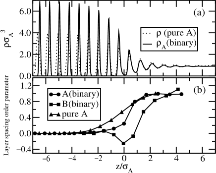
Figure 8: Comparison of the binary interface with the previously studied hard-sphere single component simulationDavidchack and Laird (1998). The upper panel shows the [100] fine scale density for both interfaces. The single component data was shifted along the $z$-axis slightly to maximize the peak overlap in the fluid phase. The lower panel shows a comparison with the lattice spacing of the [100] interface - for comparison purposes, the data is scaled and shifted (vertically) so that all curves go from zero in the crystal to unity in the fluid.)

A convenient measure of the width of the interfacial region is the so-called 10-90 width defined as the distance over which an interfacial profile changes from $10\%$ to $90\%$ of the higher of the two coexisting bulk values relative to the lower bulk value. Such a definition is only useful for those interfacial profiles which are monotonic across the interface, such as a coarse-grained (filtered) density or diffusion constants. For the filtered large particle densities the 10-90 widths are $2.6\sigma_{A}$ for the [100] and $2.4\sigma_{A}$ for the [111] - these are lower by about 0.8$\sigma_{A}$ than those found for the single component systemDavidchack and Laird (1998) which were about 3.3$\sigma$ for the two interfaces. From the small particle densities, the widths are larger at $3.4\sigma_{A}$ and $3.2\sigma_{A}$ for the [100] and [111] orientations, respectively, The 10-90 region defined by the large particles is within that defined by the small particles. The larger 10-90 width of the small particle filtered density is due to the ability of the small particles to penetrate into the first few crystal lattice layers.

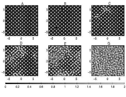
Figure 9: Cross-sectional (x-y) density distributions of the large spheres for different layers of the [100] interface.

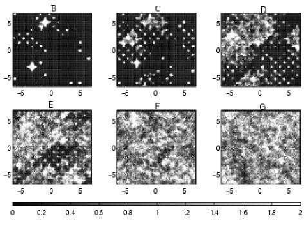
Figure 10: Cross-sectional (x-y) density distributions of the small spheres for different layers of the [100] interface.

To get a more detailed picture of the transition from crystal-like to fluid-like structure as the interface is traversed it is useful to examine the density distributions within x-y cross-sectional planes parallel to the interface. (The reported distributions are averages taken over 1800 cpp - details of their calculation can be found in the previous section.) Figures 9 and  10 respectively show the x-y large and small particle density distributions for the [100] interface orientation as greyscale contour plots. The layer labels A-G correspond to those shown in Fig. 5. Fig. 9 shows that this transition from crystal to fluid occurs over about three layers (C,D and E) for the [100] interface and that these transition layers are not uniform, but consist of coexisting solid- and liquid-like regions, as was seen in the single-component simulationsDavidchack and Laird (1998). Layer B, although fully crystalline, does possess two vacancy defects at points $(-3.3,-3.0)$ and $(-1.0,5.3)$. The [100] contour plots for the small particle density are quite interesting. There is considerable density in layer B where the small particles are present in two types of positions - in the ’NaCl’ interstitial positions and in the positions corresponding to the vacancies of the large particle crystal lattice found in layer B. The interstitial positions are occupied by single small particles, but each vacancy is filled with several small particles. In the single component simulationsDavidchack and Laird (1998) vacancy nucleation at the interface was also seen, in that case the vacancies once formed were highly mobile, migrating into the bulk via a hopping mechanism. In the present simulations, however, once the vacancies are formed in the large particle lattice, they are quickly filled with some number of small particles, which appears to immobilize the defect by suppressing the hopping mechanism - however the evidence for this is anecdotal, as the number of such vacancies is too small to gather meaningful statistics.

To estimate the degree of interfacial segregation, the Gibbs dividing surface for both interfacial orientations was determined according to Eq. 11 and found it to be close to the interface location determined from the orientational order parameters. The surface is at $z=-0.5\sigma_{A}$ for [100] and at $z=-0.9\sigma_{A}$ for [111]. At these dividing surfaces, the excess density of solute (here defined as component B) was found to be negligible - indicating minimal interfacial segregation. Of course, for such interfacial simulations, the question of complete chemical equilibrium is generally problematic, as discussed in the previous section; however, we are confident that the concentrations of each particle type from interfacial layer B out to the bulk fluid are in chemical equilibrium (since diffusion is non-negligible there) and that the equilibrium concentrations of small particles in layers deeper into the crystal are probably quite small and will not significantly affect the results presented here.

V.2 Dynamics

We study the dynamics across the interface by measuring diffusion coefficients in the coarse-scaled bins. The diffusion profiles for the [100] and [111] interfaces are shown in Figures 11(a) and  12(a), respectively.

The limiting bulk diffusion coefficient is $0.012(k_{B}T\sigma_{A}^{2}/m)^{1/2}$ for the large spheres and $0.050(k_{B}T\sigma_{A}^{2}/m)^{1/2}$ for the small particles, independent of the crystal orientation, as expected. When the three Cartesian components of the total diffusion coefficient are separately determined, it is found that diffusion is isotropic throughout the interfacial region.

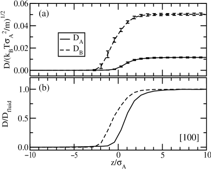
Figure 11: (a) Diffusion coefficient profile for the [100] interface. (b) Scaled diffusion coefficients.

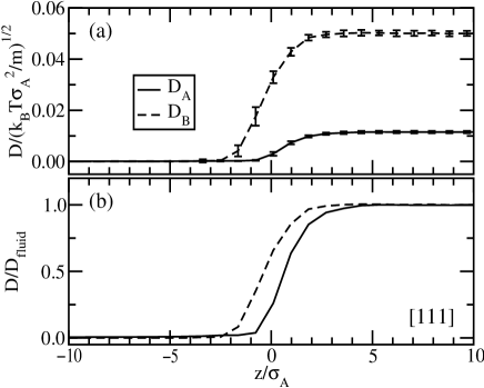
Figure 12: (a) Diffusion coefficient profile for the [111] interface. (b) Scaled diffusion coefficients.

The larger value of the small particle diffusion constant makes it difficult to compare the diffusion constants of the two components so we also plot for each, the ratio diffusion constant to the average fluid bulk value in Figures 11(b) and  12(b). Here we find the interesting result that the two curves (for both crystal orientations) are similar in shape, but shifted relative to one another by more than 1$\sigma_{A}$. As the interface is traversed from fluid to crystal, the diffusion constant for the large particle goes effectively to zero near $z=0$, but the small particles still have significant mobility. In this region, the large particles have become “locked in” to their crystal lattice sites, but the small particles can still move about - primarily by hopping between interstitial sites.

The 10-90 widths from the diffusion coefficient profiles for both orientation and particle types are about $3\sigma_{A}$. But because the diffusion profiles are shifted, the 10-90 widths do not define the same region. If contributions from both particle types are considered, the widths are $4.5\sigma_{A}$ for the [100] and $3.9\sigma_{A}$ for the [111] interface. The center of these interfacial regions are shifted by about $1\sigma_{A}$ to the fluid side compared to the interfacial regions defined by the density profiles. To illustrate this more clearly, we show in Fig. 13 all of the order parameter profiles (orientation, diffusion and density) for the [100] interface, scaled in such a way that they go from unity in the crystal phase to zero in the liquid (for example for the diffusion constants we plot $1-D(z)/D_{f}$).

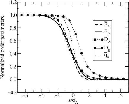
Figure 13: Diffusion, orientation and filtered density order parameter profiles for the [100] interface - all scaled such that they go from unity in the crystal to zero in the fluid phase.

The 10-90 regions for the diffusion constants are offset (toward the liquid side) from those for the filtered density profiles so the interfacial region is wider than any single structural or dynamical quantity would indicate. If one considers the interfacial region as the union of the 10-90 regions for the separate profiles, then the width of the interfacial region is $4.8\sigma_{A}$, greater than that calculated from densities or diffusion coefficients alone.

VI Summary

We have performed a series of molecular-dynamics simulations to study the crystal-melt interface of a binary hard-sphere system with diameter ratio 0.414. Previous simulation studies on two-component crystal-melt interfaces have focused on equilibrium between a fluid mixture and a substitutionally disordered crystalDavidchack and Laird (1996, 1999), but here we have examined the interface between a fluid mixture (approximately equimolar in concentration) and a coexisting single-component fcc crystal comprised of large particles - in which the small particles are immiscible. Such a coexistence occurs at relatively low pressures in the phase diagram for this diameter ratio - at higher pressures the fluid coexists with a 1:1 ordered crystal with an ‘NaCl’ structure. At a pressure of $P=20.1\sigma_{A}^{3}/kT$ the two phases coexist at the following packing fractions: $\eta_{c}=0.61$ and $\eta_{f}=0.51$.

Some of the principal results of this study are as follows:

• The interfacial density profiles of the large particles is very similar to that of the single-component hard-sphere system previously studiedDavidchack and Laird (1998), indicating that the presence of the small particle has no significant effect on the interfacial structure of the large particle, except for a compression of the crystal lattice due to the higher pressure. In particular the variation of the spacing between the large particle density peaks is very similar to that found in the single component studies.

• Within the regions of the interface in which the large particles are largely confined to fcc lattice sites, the small particles occupy either vacancy sites in the fcc lattice or ‘NaCl’ interstitial sites. The interstitial sites are single occupied whereas the vacancy sites are found to be occupied by several small particles. The presence of the small particles greatly suppresses the mobility of the fcc vacancies relative to those previously noted in single-component hard-sphere simulationsDavidchack and Laird (1998).

• There does not appear to be significant solute (small particle) segregation at the interface.

• The diffusion profiles of the small and large particles are similar in width (about 3 $\sigma_{A}$), but are shifted relative to one another by about 1 $\sigma_{A}$ along the interface normal ($z$ axis). As one traverses the interface from bulk fluid to bulk crystal, the diffusion constant goes to zero for the large particles in a region in which there is still significant small particle mobility. The picture in this region is of large particles localized at fcc lattice sites, with the small particles still diffusing between interstitial site within the lattice of large particles.

• As was found in previous hard-sphere interface studiesDavidchack and Laird (1998, 1999) the total width of the interfacial region is greater than the width determined by any single interfacial profile (such as diffusion or density) as the profiles for the individual quantities can be significantly shifted from one another. Specifically we see that as one moves from the crystal into the fluid the bulk density relaxes first to liquid-like values before significant mobility (diffusion) is observed. Considering both structural and dynamic properties, the interfacial (10-90) width is $4.8\sigma_{A}$.

VII Acknowledgements

We gratefully acknowledge R.L. Davidchack for helpful conversations, as well as the Kansas Center for Advanced Scientific Computing for the use of their computer facilities. We also would like to thank the National Science Foundation for generous support under grant CHE-9500211.

References

- (1) Author to whom correspondence should be addressed.
- Woodruff (1973) D. Woodruff, The Solid-Liquid Interface (Cambridge University Press, London, 1973).
- Tiller (1991) W. Tiller, The Science of Crystallization: Microscopic Interfacial Phenomena (Cambridge University Press, New York, 1991).
- Howe (1997) J. Howe, Interfaces in Materials (John Wiley & Sons, New York, 1997).
- Adamson and Gast (1997) A. Adamson and A. Gast, Physical Chemistry of Surfaces (Wiley-Interscience, New York, 1997).
- Laird (1998) B. Laird, in Encyclopedia of Computational Chemistry, edited by P. Schleyer, N. Allinger, T. Clark, P. Kollman, and H. Schaefer (J. Wiley and Sons, New York, 1998).
- Kyrlidis and Brown (1995) A. Kyrlidis and R. Brown, Phys. Rev. E 51, 5832 (1995).
- Mori et al. (1995) A. Mori, R. Manabe, and K. Nishioka, Phys. Rev. E 51, R3831 (1995).
- Davidchack and Laird (2000) R. Davidchack and B. Laird, Phys. Rev. Lett. 85, 4751 (2000).
- Broughton and Gilmer (1986) J. Broughton and G. Gilmer, J. Chem. Phys. 84, 5759 (1986).
- Galejs et al. (1989) R. Galejs, H. Raveche, and G. Lie, Phys. Rev. A 39, 2574 (1989).
- Karim and Haymet (1988) O. Karim and A. Haymet, J. Chem. Phys. 89, 6889 (1988).
- Karim et al. (1990) O. Karim, P. Kay, and A. Haymet, J. Chem. Phys. 92, 4634 (1990).
- Hayward and Haymet (2001) J. Hayward and A. Haymet, J. Chem. Phys. 114, 3713 (2001).
- Abraham and Broughton (1986) F. Abraham and J. Broughton, Phys. Rev. Lett. 56, 734 (1986).
- Landman et al. (1986) U. Landman, W. Luedtke, R. Barnett, C. Cleveland, M. Ribarsky, E. Arnold, S. Ramesh, H. Baumgart, A. Martinez, and B. Khan, Phys. Rev. Lett. 56, 155 (1986).
- Jesson and Madden (2001) B. Jesson and P. Madden, J. Chem. Phys. 113, 5935 (2001).
- Hoyt et al. (2001) J. Hoyt, M. Asta, and A. Karma, Phys. Rev. Lett 86, 5530 (2001).
- Davidchack and Laird (1999) R. Davidchack and B. Laird, Mol. Phys. 97, 833 (1999).
- Davidchack and Laird (1996) R. Davidchack and B. Laird, Phys. Rev. E 54, R5905 (1996).
- Laird (2001) B. Laird, J. Chem. Phys. 115, 2889 (2001).
- Trizac et al. (1997) E. Trizac, M. D. Eldridge, and P. A. Madden, Mol. Phys. 90, 675 (1997).
- Cottin and Monson (1995) X. Cottin and P. A. Monson, J. Chem. Phys. 102, 3354 (1995).
- Davidchack and Laird (1998) R. Davidchack and B. Laird, J. Chem. Phys. 108, 9452 (1998).
- Press et al. (1992) W. Press, S. Teukolsky, W. Vetterling, and B. Flannery, Numerical Recipies in Fortran (Cambridge University Press, New York, 1992).
- Rappaport (1995) D. C. Rappaport, The Art of Molecular Dynamics Simulation (Cambridge University Press, New York, 1995).
- Frenkel (1996) D. Frenkel and B. Smit, Understanding Molecular Simulation (Academic Press, New York, 1996).