K-calculus in 4-dimensional optics

Abstract

4-dimensional optics is based on the use 4-dimensional movement space, resulting from the consideration of the usual 3-dimensional coordinates complemented by proper time. The paper uses the established K-calculus to make a parallel derivation of special relativity and 4-dimensional optics, allowing a real possibility of comparison between the two theories. The significance of proper time coordinate is given special attention and its definition is made very clear in terms of just send and receive instants of radar pulses. The 4-dimensional optics equivalent to relativistic Lorentz transformations is reviewed.

Special relativity and 4-dimensional optics are also compared in terms of Lagrangian definition of worldlines and movement Hamiltonian. The final section of the paper discusses simultaneity through the solution of a two particle head-on collision problem. It is shown that a very simple graphical construction automatically solves energy and momentum conservation when the observer is located at the collision position. A further discussion of the representation for a distant observer further clarifies how simultaneity is accommodated by 4DO.

Keywords: K-calculus; alternative theories; 4-dimensional optics; special relativity.

1 Introduction

In recent times the author has written several papers on the subject of his proposed alternative to general relativity, [1, 2, 3, 4, 5] all of them rejected by the journals to which they were submitted; refs. [1] and [2] were accepted as posters in conferences. The main reason for rejection can be found in the words of one referee:

The foundation of the author’s model is inconsistent with SR (special relativity). In particular, he gives no compelling reason why we should abandon SR which is a highly successful theory. Just to turn to an alternative speculation since, according to the author, SR is too complicated, is no sufficient reason. Therefore I have no option but to suggest to the editor of the … to reject this paper.

One should therefore ask why any effort should be made to set up an alternative to an existing theory that has proven so successful. There are at least two reasons to do so: In the first place any theory is just as good as the predictions it allows for observable phenomena and if two competing theories allow the same predictions they are equally good until some phenomenon is better predicted by one of them. Until one is proven better than the other, the coexistence of the two theories allows different perspectives which can only enhance our understanding of the underlying physics. Secondly general relativity has failed to explain properly a number of phenomena, see for instance [6], while people keep trying to merge it with the other main physical theory, the standard model. This suggests that there may be some other theory that unifies everything, the most successful so far being string theory [7].

The field is wide open for new ideas that combine the best of general relativity and the standard model, proving capable of predictions as accurate as those provided by these two theories but somehow having an entirely different approach. One must always keep in mind that any model or theory is just a representation of reality and not reality itself, the latter being rather difficult to define without resorting to the observer’s own perception. In the present paper the author adopts an approach to his theory based on the K-calculus by Herman Bondi [8], which has been so successful in introducing relativity to undergraduates all over the world. In his previous works the author used a different approach and he hopes that this effort may render the theory more acceptable to those that have difficulty accepting that there may be alternatives to relativity. Furthermore there issues related to simultaneity which have not been addressed so far and are clarified in the present work.

The coordinate system used in 4-dimensional optics, henceforth referred to as 4DO, differs from the relativistic space-time in complementing the 3 spatial coordinates ($x^{1}=x$, $x^{2}=y$, $x^{3}=z$) with a 0th coordinate ($x^{0}=\tau$) such that time becomes a measure of geodesic arc length in Euclidean space. Using the usual simplification of making $c=1$,

$$\left(\mathrm{d}t\right)^{2}=\left(\mathrm{d}\tau\right)^{2}+\left(\mathrm{d}x\right)^{2}+\left(\mathrm{d}y\right)^{2}+\left(\mathrm{d}z\right)^{2}.$$ (1)

This equation is valid on tangent space only; for the more general situation of curved space the definition is extended as

$$\left(\mathrm{d}t\right)^{2}=g_{\alpha\beta}\mathrm{d}x^{\alpha}\mathrm{d}x^{\beta},$$ (2)

with $g_{\alpha\beta}$ the movement metric, rather than the space metric as in general relativity [4, 5].

Understanding the meaning of coordinate $\tau$ is crucial for proper handling of the theory in the most general situations, so it was felt necessary to develop the basic theory in a way similar to what is usually used to introduce relativity in undergraduate courses, thereby giving the reader a good means for assessing the similarities and differences between the two theories. The author chooses to follow an introductory path closely similar to what was introduced by Bondi [8] and later used by other authors, namely Martin [9] and D’Inverno [10]. For an observer traveling at speed $v$, Bondi introduced the $K$ factor

$$K=\sqrt{\frac{c+v}{c-v}}\,,$$ (3)

which has since been used to identify this approach as K-calculus.

It is useful to remember that in 4DO the speed as we see it, what will be designated by 3-speed, is actually the 3-dimensional component of a 4-vector with the magnitude of the speed of light. This was first explained in an introductory work by the author [1] and later developed in the works cited previously. This approach ensures that 3-speed is bound by the speed of light without resorting to hyperbolic space, as is the case in relativity. Besides, it has been shown that 4DO holds the potential for explaining physical processes which relativity has failed to account for satisfactorily.

2 Coordinate definition

Bondi resorts to imaginary radar pulses bouncing on a distant observer and a clock for the definition of space and time coordinates. The idea is that the observer fixed on the laboratory frame investigates the space around him with the help of radar pulses and a clock. When a radar pulse is sent the observer records the send instant $\tau_{1}$ and when the echo is received from some location in space the observer records the receive instant $\tau_{3}$ and the direction angles $\theta$ and $\phi$; the reflection instant $\tau_{2}$ is inaccessible to the observer. The direction angles provide two of the position coordinates; remembering that the speed of light is set to unity, the third position coordinate is the distance to the reflecting object

$$r=\frac{\tau_{3}-\tau_{1}}{2}\,.$$ (4)

The time coordinate is naturally given by

$$t=\frac{\tau_{3}+\tau_{1}}{2}\,.$$ (5)

Conversely 4DO replaces the time coordinate with a coordinate defined by the reflection instant

$$\tau=\tau_{2}.$$ (6)

The locus of an observer’s points in either space is said to define the observer’s worldline in that particular space. The graphical representation of 4-dimensional spaces is difficult, so it is usual to suppress two spatial dimensions in order to represent a 2-dimensional section of the space or to suppress one spatial dimension and project the resulting 3-dimensional section on the plane as a perspective diagram; this paper uses mainly the 2-dimensional section representation.

Suppose now an observer moving with uniform velocity $v$ in the laboratory frame. This observer’s worldline is a straight line on both systems and for convenience it can be assumed that it passes through the coordinate origin. In 2 dimensions the observer’s worldline has an equation $x=vt$; using Eqs. (4, 5) one can write

$$\tau_{3}-\tau_{1}=v\left(\tau_{3}+\tau_{1}\right),$$ (7)

which leads to the relation

$$\tau_{3}=\frac{1+v}{1-v}~{}\tau_{1}.$$ (8)

Considering the K-factor definition, Eq. (3), it is

$$\tau_{3}=\tau_{1}K^{2}.$$ (9)

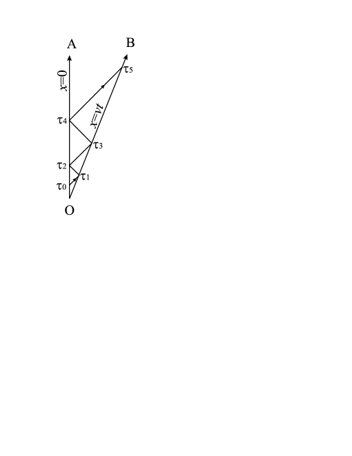
Figure 1: Minkowski space-time representation: Inertial observer B moves with relative velocity $v$ with respect to observer A. Observer A launches a radar pulse at instant $\tau_{0}$, which bounces back and forth between the two observers.

Two inertial observers A and B are now considered, the latter moving with velocity $v$ relative to A. Fig. 1 shows the Minkowski space-time worldlines of the two observers as two straight lines diverging from the origin. The origin placement at the point of intersection of the two worldlines does not represent any limitation on the problem conditions. At instant $\tau_{0}$ observer A launches a radar pulse which is bounced back and forth successively between the two observers. The radar pulse moves at the speed of light with respect to both observers so, in observer A’s frame its worldline is a broken line with alternating segments of slope $+1$ and $-1$, respectively. The radar pulses worldlines follow the general equation $t=\pm x+\tau_{2m-2}$, with $m$ integer.

Observe that the $K$-factor is the same for both observers and so it is possible to write Eq. (8) generally as

$$\tau_{n+1}=\frac{1+v}{1-v}~{}\tau_{n-1}=\tau_{n-1}K^{2}.$$ (10)

The last equation defines recursively a succession of general term

$$\tau_{n}=\tau_{0}K^{n}.$$ (11)

It is now possible to use Eq. (11) as an alternative to Eq. (6) for the definition of the $\tau$ coordinate

$$\tau_{n}=\sqrt{\tau_{n+1}\tau_{n-1}}.$$ (12)

Comparing with Eq. (5) it becomes clear that while Minkowski space-time defines time as the arithmetic mean between the send and receive instants, 4DO uses a coordinate defined as the geometric mean between the same instants for $\tau$. This coordinate will be designated proper time in view of its relationship with the similarly designated quantity in relativistic theory [4].

Eq. (5) can be used to relate $t_{n}$ and $\tau_{n}$ eliminating $\tau_{n+1}$ and $\tau_{n-1}$ from the following three equations:

$$\tau_{n}=K\tau_{n-1},~{}~{}\tau_{n+1}=K\tau_{n},~{}~{}t_{n}=\frac{\tau_{n+1}+\tau_{n-1}}{2},$$

resulting in

$$t_{n}=\gamma\tau_{n},$$ (13)

where

$$\gamma=\frac{K+K^{-1}}{2}=\frac{1}{\sqrt{1-v^{2}}}.$$ (14)

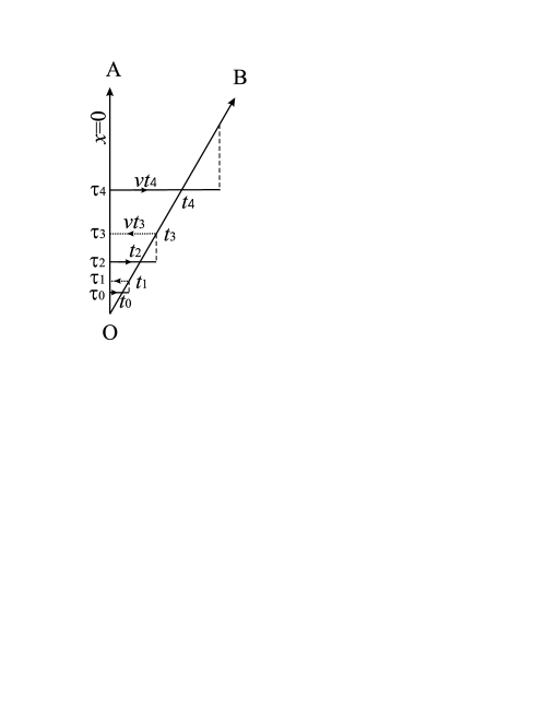
Figure 2: In optical space the observers move with velocity $c$ across 4-dimensional space and time is measured along the worldline.

Eqs. (12 or 13) allow the construction of a graphic representation for the two observers’ 4DO worldlines using coordinates $x,\tau$. Observer A’s worldline is drawn as the $\tau$ axis, because this observer does not move in his own frame. For observer B it is sufficient to plot the successive pairs $(x_{n},\tau_{n})$ and join them by a straight line; B worldline’s slope is $\tau_{n}/x_{n}$ and considering Eq. (13) it is easily seen that this slope is given by $\gamma/v$. Obviously light and radar pulses have $v=1$ and must be represented by horizontal lines of zero slope.

The final graph is shown in Fig. 2 but the interaction between radar pulses and observers needs some explanation. When the two observers leave the origin they have synchronous clocks; time, however, is then evaluated separately over each observer’s worldline. When A launches the first radar pulse, at instant $\tau_{0}$, the pulse is synchronous with A’s clock and evaluates time over it’s own worldline. The pulse’s time is compared with B’s own time at every point along the way; only when they coincide can interaction occur and this happens beyond the crossing point of the two worldlines on the graph. On B’s frame the interaction instant $t_{1}$ is translated into the proper time $\tau_{1}$; this is represented by a dashed vertical line joining the pulse’s and B’s worldlines.

The reflected pulse must suffer a similar process, only the roles of observers A and B are now interchanged. The dashed lines representing the reflected pulses at $\tau_{1}$ and $\tau_{3}$ must not be mistaken by these pulses worldlines, because they are the representation of worldlines on B’s frame. On A’s frame the instants $\tau_{1}$ and $\tau_{3}$ are inaccessible and the pulses actually return at $\tau_{2}$ and $\tau_{4}$, respectively.

From Eqs. (13 and 14) it is clear that $\tau_{n}$, $vt_{n}$ and $t_{n}$ are the sides of a rectangular triangle. Remembering that $x_{n}=vt_{n}$, it is possible to write

$$t^{2}=\tau^{2}+x^{2}.$$ (15)

The subscripts have been suppressed because the relation most hold for pulses sent out irrespective of the particular initial instant $\tau_{0}$.

A simple geometrical construction can be used to plot the points of the moving observer’s worldline, Fig. 3.

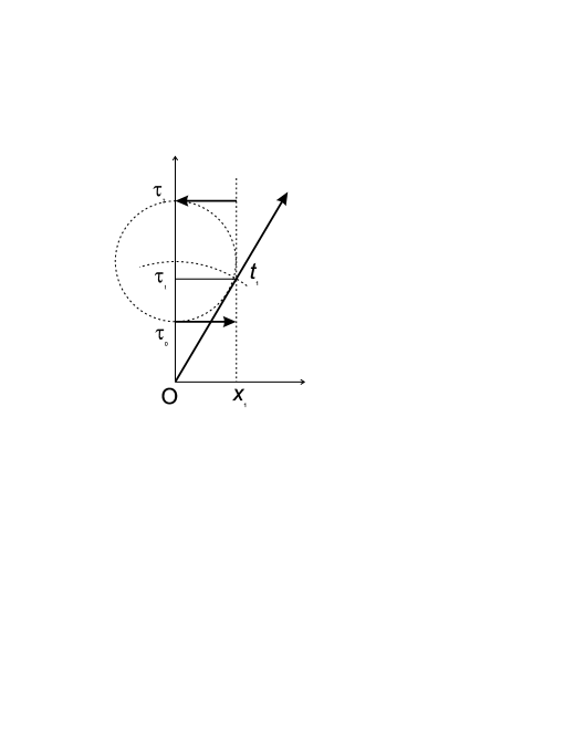
Figure 3: The figure shows a geometrical construction suitable for determining the worldline of a moving observer.

If a radar pulse is sent at $\tau_{o}$ and its reflection is received at $\tau_{2}$, a circle is drawn with diameter $\tau_{2}-\tau_{0}$ and, according to Eq. (4), the moving observer is at a distance $x_{1}$ equal to the circle radius. Considering Eq. (5) the time $t_{1}$ for the moving observer is equal to the distance from the origin to the center of the circle. A new circle is now drawn with center at the origin and radius equal to the value of $t_{1}$, in order to transport this value to the moving observer’s position. The value of coordinate $\tau_{1}$ is automatically found by the intersection of the second circle with the vertical line at position $x_{1}$. The same process can then be repeated for all the pairs of sent, received pulses.

3 Interval

Consider now how two different inertial observes ”see” a third one. Fig. 4 a)

             

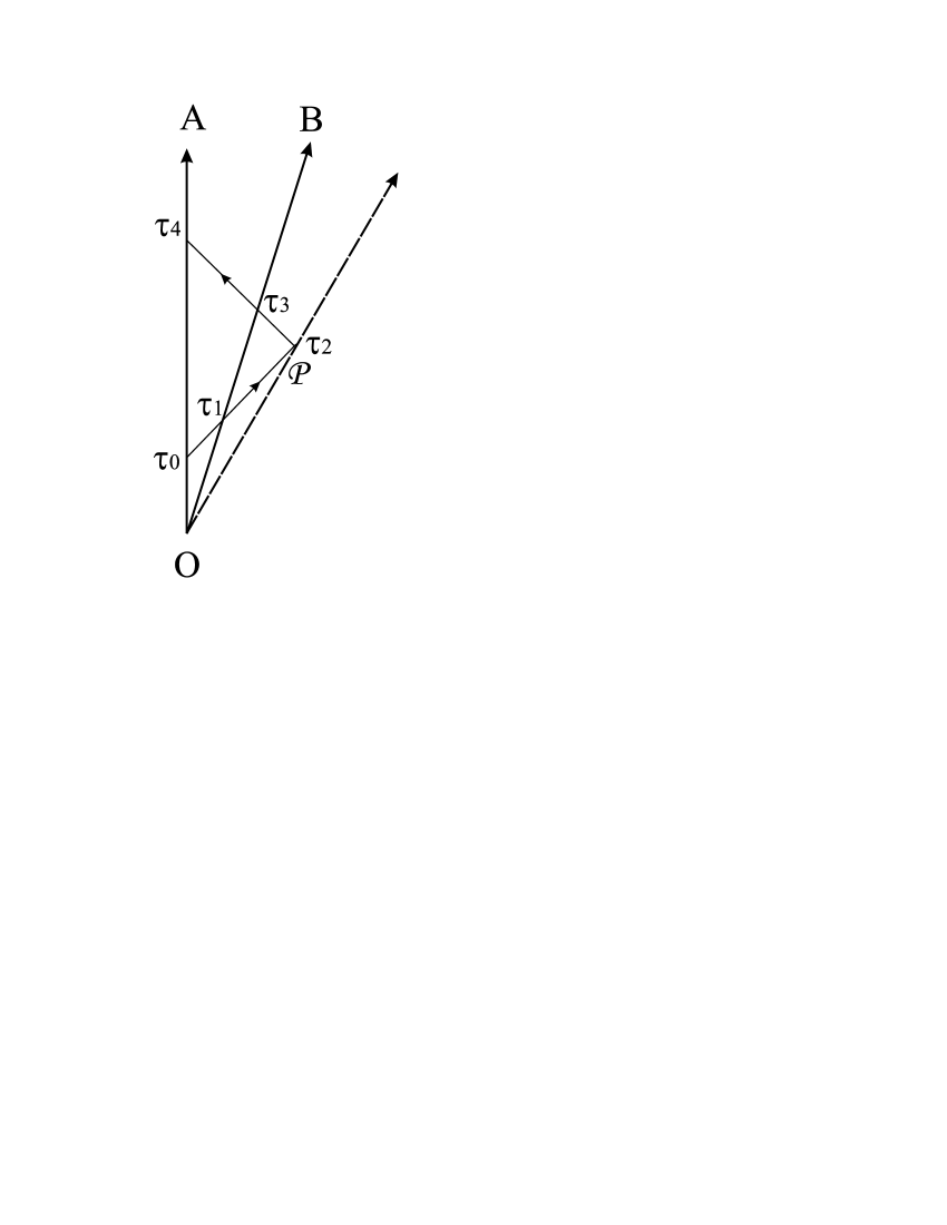
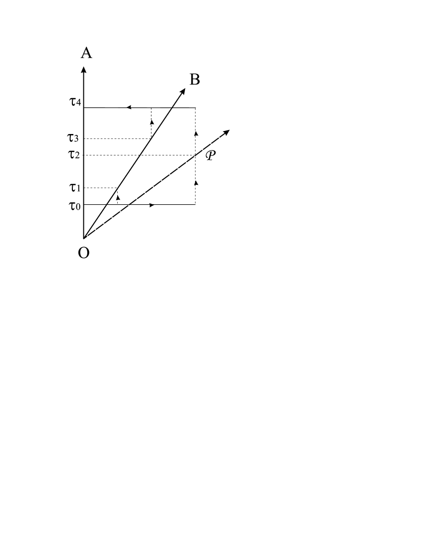
a)                                         b)

Figure 4: a) Minkowski space-time representation of two different observers looking at a third one ($\mathcal{P}$). A radar pulse is launched by observer A at instant $\tau_{0}$, passes B at instant $\tau_{1}$ and is reflected by $\mathcal{P}$ at instant $\tau_{2}$; on the way back it passes B at $\tau_{3}$ and arrives at A at instant $\tau_{4}$. b) The same situation in 4DO space.

is a Minkowski space-time representation of the worldlines of two observers A and B, B moving with speed $v$ relative to A, and a third observer $\mathcal{P}$, moving with speed $u$ relative to B. The first two observers use the radar formulas (4, 5, 12) to compute $\mathcal{P}$’s coordinates. Note first of all that

$$\frac{\tau_{1}}{\tau_{0}}=K_{v},~{}~{}\frac{\tau_{2}}{\tau_{1}}=K_{u},~{}~{}\frac{\tau_{3}}{\tau_{2}}=K_{u},~{}~{}\frac{\tau_{4}}{\tau_{3}}=K_{v}.$$ (16)

The coordinates of $\mathcal{P}$ evaluated by the two observers are

$$\begin{array}[]{ll}x_{A}=(\tau_{4}-\tau_{0})/2,{}&x_{B}=(\tau_{3}-\tau_{1})/2,\\ t_{A}=(\tau_{4}+\tau_{0})/2,{}&t_{B}=(\tau_{3}+\tau_{1})/2,\\ \tau_{A}=\sqrt{\tau_{0}\tau_{4}},{}&\tau_{B}=\sqrt{\tau_{1}\tau_{3}}~{}.\end{array}$$ (17)

by direct replacement of $\tau_{1}$ and $\tau_{3}$ from Eqs. (16) it is possible to conclude that $\tau_{A}=\tau_{B}=\tau_{2}$, i. e. the proper time coordinate is independent of the inertial observer’s own speed, as long as its worldline passes through the origin. This conclusion can be seen as equivalent to interval invariance in Minkowski space-time [9] .

The representation of Fig. 4 b) shows how the situation discussed above appears in 4DO space. The outgoing pulse at $\tau_{0}$ is detected by observer B at $\tau_{1}$ and by $\mathcal{P}$ at $\tau_{2}$. The return pulse is sent by $\mathcal{P}$ at $\tau_{2}$ but is here represented by its worldline in the laboratory frame, at $\tau_{4}$, unlike Fig. 2. Observer B detects the return pulse at $\tau_{3}$.

It is possible to combine Eqs. (16 and 17) to obtain

$$t_{A}^{2}=\tau_{A}^{2}+x_{A}^{2},~{}~{}t_{B}^{2}=\tau_{B}^{2}+x_{B}^{2}.$$ (18)

Eqs. (18) mean that the quantity $t^{2}$ can be evaluated as $\tau^{2}+x^{2}$ by any observer whose worldline passes by the origin. If the problem is given a more general formulation, in 4 dimensions and without the restriction of the worldlines having to cross at the origin, it can be said that

$$\left(\mathrm{d}t\right)^{2}=\delta_{\alpha\beta}\mathrm{d}x^{\alpha}\mathrm{d}x^{\beta},$$ (19)

which is equivalent to saying that time is a measure of geodesic arc length in Euclidean 4DO space.

The important results are then: 4DO space is Euclidean, with time intervals being measured over the worldline of the observer. In a change of coordinates from one observer to a different one, which is in motion relative to the former, time intervals are not preserved but rather proper time intervals.

In Minkowski space-time it is well known that the interval is preserved in coordinate transformations and is given by [9, 10]

$$\left(\mathrm{d}\tau\right)^{2}=\eta_{\bar{\alpha}\bar{\beta}}\mathrm{d}x^{\bar{\alpha}}\mathrm{d}x^{\bar{\beta}},$$ (20)

with

$$\begin{array}[]{ll}\eta_{\bar{\alpha}\bar{\beta}}=1,&\bar{\alpha}=\bar{\beta}=0;\\ \eta_{\bar{\alpha}\bar{\beta}}=-1,&\bar{\alpha}=\bar{\beta}\neq 0;\\ \eta_{\bar{\alpha}\bar{\beta}}=0,&\bar{\alpha}\neq\bar{\beta}.\end{array}$$ (21)

for the set of coordinates

$$x^{0}=t,~{}~{}x^{1}=x,~{}~{}x^{2}=y,~{}~{}x^{3}=z.$$ (22)

The bar over the indices is here used to designate Minkowski space-time coordinates.

Eqs (18 and 20) provide the rules for elementary displacement transformation when changing from one space to the other. Assume that the vector $\mathrm{d}x^{\bar{\alpha}}$ is expressed in Minkowski space-time and must be transformed to 4DO space; the transformation rule is

$$\begin{array}[]{ll}\mathrm{d}x^{\alpha}=\sqrt{\eta_{\bar{\mu}\bar{\nu}}\mathrm{d}x^{\bar{\mu}}\mathrm{d}x^{\bar{\nu}}},&\alpha=0;\\ \mathrm{d}x^{\alpha}=\mathrm{d}x^{\bar{\mu}},&\alpha=\bar{\mu}\neq 0.\end{array}$$ (23)

The opposite transformation follows a similar rule

$$\begin{array}[]{ll}\mathrm{d}x^{\bar{\alpha}}=\sqrt{\delta_{\mu\nu}\mathrm{d}x^{\mu}\mathrm{d}x^{\nu}},&\bar{\alpha}=0;\\ \mathrm{d}x^{\bar{\alpha}}=\mathrm{d}x^{\mu},&\bar{\alpha}=\mu\neq 0.\end{array}$$ (24)

It is possible to define the 4-velocity for an observer in the two spaces as $\dot{x}^{\alpha}=\mathrm{d}x^{\alpha}/\mathrm{d}t$ and $\dot{x}^{\bar{\alpha}}=\mathrm{d}x^{\bar{\alpha}}/\mathrm{d}t$, respectively, with the $t$ derivatives taken over the worldline. The 4-velocity transformation between the two spaces follows rules similar to those expressed by Eqs. (23, 24) with $\mathrm{d}x^{\bar{\alpha}}$ and $\mathrm{d}x^{\alpha}$ replaced by $\dot{x}^{\bar{\alpha}}$ and $x^{\alpha}$.

4 Lorentz equivalent transformations

The subject of this paragraph has already been considered in [4] but needs to be reviewed here for completeness. Our approach to coordinate transformation between observers moving relative to each other is different from special relativity; while in the latter case the interval is given by Eq. (20), thus ensuring that a coordinate transformation preserves the interval and affects both spatial and time coordinates, our option of making time intervals measure geodesic arc length gives time a meaning independent of any coordinate transformation. We thus propose that Lorentz equivalent transformations between a ”fixed” or ”laboratory” frame and a moving frame are a combination of two simultaneous processes. The first process is a tensorial coordinate transformation, which changes the coordinates keeping the origin fixed, with no influence in the way time is measured, while the second process corresponds to a ”jump” into the moving frame, changing the metric but not the coordinates.

It has been established in page 2 that photons follow worldlines of $\mathrm{d}\tau=0$ and carry the value of the $\tau$ coordinate across the Universe, which was confirmed in page 17 by the verification that proper time intervals were independent of the observer. On the other hand the time interval must also evaluate to the same value on all coordinate systems of the same frame, due to its definition as interval of 4DO space.

One can consider observers $O$ and $\bar{O}$, the latter moving along one geodesic of $O$’s coordinate system, as depicted in Fig. 5. Let the geodesic equation have a parametric equation $x^{\alpha^{\prime}}(t)$. The aim is to to find a coordinate transformation tensor between the two observers’ coordinate systems, ${\Lambda^{\bar{\mu}}}_{\alpha}=\partial x^{\bar{\mu}}/\partial x^{\alpha}$; it has already established that $\mathrm{d}x^{\bar{0}}=\mathrm{d}x^{0}$ and so it must be ${\Lambda^{\bar{0}}}_{0}=1$ and ${\Lambda^{\bar{0}}}_{i}=0$.

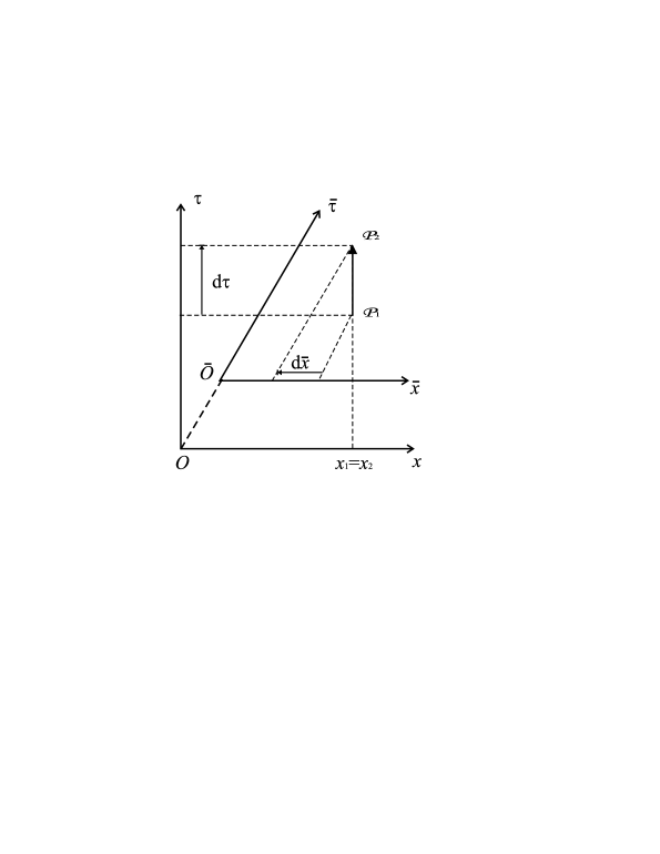
Figure 5: The worldline of moving observer $\bar{O}$ coincides with the $\bar{\tau}$ or $x^{\bar{0}}$ axis, while the $\bar{x}$ axis stays parallel to the $x$ axis. A displacement parallel to axis $\tau$ or $x^{0}$ implies both $\bar{x}$ and $\bar{\tau}$ components in the moving frame.

A photon traveling parallel to the $x^{1}$ direction follows a geodesic characterized by $\mathrm{d}t=\mathrm{d}x^{1}$ on $O$’s coordinates. On $\bar{O}$’s coordinates the photon will move parallel to $x^{\bar{1}}$ and so it must be also $\mathrm{d}t=\mathrm{d}x^{\bar{1}}$. The same behaviour could be established for all three $(x^{i},~{}x^{\bar{i}})$ coordinate pairs and one concludes that ${\Lambda^{i}}_{\bar{i}}=1$.

Consider now two points $\mathcal{P}_{1}$ and $\mathcal{P}_{2}$ on a line parallel to $x^{0}$ axis in $O$’s coordinates, separated by a time interval $\mathrm{d}t=\mathrm{d}x^{0}$. On $\bar{O}$’s coordinates it will be

$$\mathrm{d}x^{\bar{i}}=-\dot{x}^{i^{\prime}}\mathrm{d}t=-\frac{\dot{x}^{i^{\prime}}}{\dot{x}^{0^{\prime}}}~{}\mathrm{d}x^{0},$$ (25)

allowing the conclusion that ${\Lambda^{\bar{i}}}_{0}=-\dot{x}^{i^{\prime}}/\dot{x}^{0^{\prime}}=-\breve{x}^{i}$, where the notation $\breve{x}^{i}$ is used for derivation with respect to $\tau$. Fig. 5 shows graphically the relation between the two coordinate systems.

The coordinate transformation tensor between $x^{\alpha}$ and $x^{\bar{\mu}}$ is consequently defined as

$${\Lambda^{\bar{\mu}}}_{\alpha}=\left[\begin{array}[]{cccc}1&0&0&0\\ -\breve{x}^{1^{\prime}}&1&0&0\\ -\breve{x}^{2^{\prime}}&0&1&0\\ -\breve{x}^{3^{\prime}}&0&0&1\end{array}\right].$$ (26)

The reverse transformation is obtained changing the sign of $-\breve{x}^{i}$.

The metric for $\bar{O}$’s coordinates can now be evaluated

$$g_{\bar{\mu}\bar{\nu}}={\Lambda^{\alpha}}_{\bar{\mu}}{\Lambda^{\beta}}_{\bar{\nu}}g_{\alpha\beta};$$ (27)

and after substitution it is

$$g_{\bar{\mu}\bar{\nu}}=\left[\begin{array}[]{cccc}1+\delta_{a^{\prime}b^{\prime}}\breve{x}^{a^{\prime}}\breve{x}^{b^{\prime}}&\breve{x}^{1^{\prime}}&\breve{x}^{2^{\prime}}&\breve{x}^{3^{\prime}}\\ \breve{x}^{1^{\prime}}&1&0&0\\ \breve{x}^{2^{\prime}}&0&1&0\\ \breve{x}^{3^{\prime}}&0&0&1\end{array}\right].$$ (28)

The metric given by the previous equation will evaluate time in $\bar{O}$’s coordinates in a frame which is fixed relative to $O$, that is, this is still time as measured by observer $O$. Observer $\bar{O}$ will measure time intervals $\mathrm{d}\bar{t}$ in his own frame and so, although the coordinates are the same as they were in $O$’s frame, time is evaluated with the Kronecker metric $\delta_{\bar{\mu}\bar{\nu}}$ instead of metric given by Eq. (28). Mathematically the metric replacement corresponds to the identity

$$\delta_{\bar{\alpha}\bar{\beta}}=\left(g_{\bar{\mu}\bar{\nu}}\right)^{-1}g_{\bar{\mu}\bar{\nu}}.$$ (29)

It was said in page 4 that the transition from the laboratory frame to a moving observer’s frame was the result of two separate processes, one of which was responsible for the change of coordinates and the other one for the time change. The first process can now be identified with a coordinate change governed by the tensor ${\Lambda^{\bar{\mu}}}_{\alpha}$, while the second one involves multiplication of the metric by $g^{\bar{\mu}\bar{\nu}}$. The second process is intrinsically separate from the first one and was used in [4, 5] to derive the Lorentz force due to a moving charge and the center of mass equivalent of an orbiting mass.

Note that this double process preserves the essential relationship of special relativity, i. e. $\mathrm{d}\bar{t}^{2}-\delta_{\bar{i}\bar{j}}\mathrm{d}x^{\bar{i}}\mathrm{d}x^{\bar{j}}=\mathrm{d}t^{2}-\delta_{ij}\mathrm{d}x^{i}\mathrm{d}x^{j}$.

4.1 Time contraction for a moving observer

Eq. (18) established that time intervals should be measured by the arc length of an observer’s worldline. Recalling Fig. 5, the time measured for observer $\bar{O}$’s trajectory in the laboratory frame of observer $O$ is given by $\mathrm{d}t=\gamma\mathrm{d}\tau$, according to Eq. (13). Observer $\bar{O}$ is at rest in his own frame and sees his frame axes normal to each other, i.e. he uses the Kronecker metric, and so he measures for himself a time interval $\mathrm{d}\bar{t}=\mathrm{d}\tau$. Obviously $\mathrm{d}\bar{t}<\mathrm{d}t$ and so we say that the time measured by a moving observer runs slower than the time measured on the laboratory frame.

At this point it is useful to give physical meaning to the coordinate $\tau$, so that 4DO is understood as a space with physical significance. This space is designed to represent the movement of observers through 3-dimensional space. Accordingly it uses the standard coordinates to identify the observers’ positions, eventually scaled by the observers’ masses as described in Refs. [4, 5]. The 0th coordinate $\tau$ does not have a Universal meaning, as was shown in the previous paragraph; it is just the time indicated by the observers’ own clocks and so it does deserve to be called proper time. The fact that coordinate $\tau$ can be identified with each observer’s own time is of no consequence for the representation of his own worldline but becomes important when two observers interact, for then time must evaluate to the same value when both observers’ worldlines are represented in a common frame. The problems of interaction between observers and the concept of simultaneity will be dealt with in paragraph 7.

4.2 The twin paradox in optical space

It is customary to discuss the case of two twins $A$ and $B$, of which $A$ stays at home, remaining inertial at all times, while $B$ goes on an extended space flight at high speed before he eventually joins $A$ back home. The reasoning is that as $B$’s time is constantly running slower than $A$’s, $B$ must come back younger than $A$.

In 4DO the argument is inconsistent because one must distinguish between the time measurements on the frames of the two twins. In fact $B$’s time measured on his own frame is shorter than his time measured by $A$ on the fixed frame. On the other hand $B$’s time measured by himself is exactly the same as $A$’s time measured on the fixed frame and the two twins actually grow old together. A proper discussion of this problem should not ignore the fact that $B$’s frame is necessarily accelerated and this has also an influence on the way clocks run.

5 Lagrangean definitions for geodesics in Minkowski and 4DO

If $\sigma$ is a parameter along a geodesic, for any space the geodesic equations can be derived from the Lagrangean [9]

$$L\left(x^{\alpha},\frac{\mathrm{d}x^{\alpha}}{\mathrm{d}\sigma}\right)=g_{\alpha\beta}\frac{\mathrm{d}x^{\alpha}}{\mathrm{d}\sigma}\frac{\mathrm{d}x^{\beta}}{\mathrm{d}\sigma}.$$ (30)

The geodesic equations are then

$$\frac{\mathrm{d}}{\mathrm{d}\sigma}\left(\frac{1}{\sqrt{L}}\frac{\partial L}{\displaystyle{\partial\frac{\mathrm{d}x^{\alpha}}{\mathrm{d}\sigma}}}\right)-\frac{1}{\sqrt{L}}\frac{\partial L}{\partial x^{\alpha}}=0,$$ (31)

with $n-1$ independent equations on an $n$-dimensional space. If the geodesic arc length is chosen as parameter the Lagrangean becomes unity.

It can be shown that the geodesic equations are equivalent in Minkowski and optical spaces. For this one chooses arc length as parameter in both spaces and derives the geodesic equations starting from the Lagrangean.

Considering Eq. (20), in 2-dimensional Minkowski space-time the Lagrangean is

$$L_{\mathrm{M}}=\left(\frac{\mathrm{d}t}{\mathrm{d}\tau}\right)^{2}-\left(\frac{\mathrm{d}x}{\mathrm{d}\tau}\right)^{2}=1.$$ (32)

As the Lagrangean is independent of $t$ one can write

$$\frac{\partial L_{\mathrm{M}}}{\partial\displaystyle{\frac{\mathrm{d}t}{\mathrm{d}\tau}}}=2\frac{\mathrm{d}t}{\mathrm{d}\tau}=\mathrm{constant}.$$ (33)

Making the second member of the equation above equal to $2\gamma$ and replacing in Eq. (32)

$$1=\gamma^{2}-\left(\frac{\mathrm{d}x}{\mathrm{d}\tau}\right)^{2}.$$ (34)

Noting that $\mathrm{d}x/\mathrm{d}\tau=\gamma\mathrm{d}x/\mathrm{d}t=\gamma v$

$$1=\gamma^{2}\left(1-v^{2}\right),$$ (35)

which is an equation equivalent to Eq. (14).

Considering now a 2-dimensional section of 4DO space and using again arc length as parameter, the Lagrangean is

$$L_{\mathrm{O}}=\left(\frac{\mathrm{d}\tau}{\mathrm{d}t}\right)^{2}+\left(\frac{\mathrm{d}x}{\mathrm{d}t}\right)^{2}=1.$$ (36)

The fact that the Lagrangean does not depend on $\tau$ allows one to set $\mathrm{d}\tau/\mathrm{d}t=1/\gamma$ and replace above to get

$$\frac{1}{\gamma^{2}}+v^{2}=1,$$ (37)

the same as Eq. (35).

Eqs. (34, 35) were both derived from the Lagrangeans and state the basic relationship between time and proper time that had been established before. It is then clear that both spaces are equally adequate for derivation of the geodesic equations.

Although the geodesic equations are the same in both spaces the Lagrangeans are not equivalent; when $t$ is used as parameter in Eq. (30) the Minkowski Lagrangean simplifies to $L_{\mathrm{M}}=1-v^{2}$ while the 4DO Lagrangean is still given by Eq. (36). The implications of this difference will be discussed below.

6 Hamiltonian and particle energy

The Hamiltonian of a system is a function of coordinates, conjugate momenta and a parameter, that describes the system evolution in phase space. Phase space associated with 4-dimensional coordinate space should then be 9-dimensional. In classical mechanics one is usually led to use time as parameter, thus eliminating two dimensions in phase space. What follows compares phase spaces associated with 2-dimensional sections of Minkowski and 4DO spaces.

It has been established that the Lagrangean must be unity when expressed in terms of the arc length so the action in Minkowski space-time is

$$\delta\int\mathrm{d}s=\delta\int\sqrt{(\mathrm{d}t)^{2}-(\mathrm{d}x)^{2}}=\delta\int\sqrt{1-\dot{x}^{2}}~{}\mathrm{d}t=0,$$ (38)

with ”dot” used to represent time derivative. The Lagrangean with time as parameter can then be taken as [11]

$$L_{\mathrm{M}}=\sqrt{1-\dot{x}^{2}}=\frac{1}{\gamma}~{},$$ (39)

from which it is possible to derive the conjugate momentum

$$p_{\mathrm{M}}=\frac{\partial L_{\mathrm{M}}}{\partial\dot{x}}=-\gamma\dot{x},$$ (40)

and the Hamiltonian

$$H_{\mathrm{M}}=p_{\mathrm{M}}\dot{x}-L_{\mathrm{M}}=-\frac{1}{\gamma}.$$ (41)

Eq. (41) justifies the statement that a unit mass body’s energy is given by $-1/\gamma$ and quite naturally, if the body has mass $m$ one says that the energy increases proportionally.

Looking at 4DO space one can perform a similar derivation; the action is now

$$\delta\int\mathrm{d}t=\delta\int\sqrt{(\mathrm{d}\tau)^{2}+(\mathrm{d}x)^{2}}=\delta\int{\sqrt{1+\left(\frac{\mathrm{d}x}{\mathrm{d}\tau}\right)^{2}}~{}\mathrm{d}\tau}=0.$$ (42)

from which the Lagrangean and conjugate momentum with $\tau$ as parameter can be derived

$$L_{\mathrm{O}} = \gamma=\sqrt{1+\left(\frac{dx}{d\tau}\right)^{2}},$$ (43)

$$p_{\mathrm{O}} = \frac{\partial L_{\mathrm{O}}}{\partial\tau}=\frac{1}{\gamma}\frac{\partial x}{\partial\tau}.$$ (44)

Note that $p_{\mathrm{O}}=\dot{x}/(\gamma\dot{\tau})$ and considering Eq. (13) $p_{\mathrm{O}}=\dot{x}$.

The Hamiltonian becomes

$$H_{\mathrm{O}}=p_{\mathrm{O}}\frac{\partial x}{\partial\tau}-L_{\mathrm{O}}=-\frac{1}{\gamma}.$$ (45)

It is tempting to see the fact that $H_{\mathrm{M}}=H_{\mathrm{O}}$ as a confirmation that both spaces are equivalent for the study of a body’s movement. This is actually not quite true!

The differences arise when the body is influenced by a coordinate dependent potential $V$, in which case one should write $H=-m/\gamma+V$; in Minkowski space one gets the familiar canonical equation

$$\frac{\mathrm{d}p_{\mathrm{M}}}{\mathrm{d}t}=-\frac{\partial H}{\partial x},$$ (46)

while in 4DO space it is

$$\frac{\mathrm{d}p_{\mathrm{O}}}{\mathrm{d}\tau}=\gamma\frac{\mathrm{d}}{\mathrm{d}t}\left(\frac{p_{\mathrm{M}}}{\gamma}\right)=-\frac{\partial H}{\partial x}.$$ (47)

The difference between Eqs. (46) and (47) exists only when $\gamma$ is time dependent; this happens if the velocity is varying not only in direction but also in magnitude. In fact the problem only arises because a potential was considered but it has been stated already [4] that 4DO precludes potentials and considers all interactions to be dealt with through space curvature and associated metric modification. The problem is then ill-posed; nevertheless the predictions of general relativity will not be coincident with 4DO’s whenever the former theory appeals to potentials.

7 Conservation law and simultaneity

Understanding the physical meaning of proper time is important if one wishes to acquire the feeling of the physical phenomena that are expressed in optical space. One is used to the concept of simultaneity and the discussion in section 3 has already shown that this concept is not easily translated into the new space; the following lines discuss a typical problem involving simultaneity, which hopefully will clarify this point. A collision situation is as good as one can get to discuss simultaneity, with the bonus that it will bring conservation into the picture.

First of all it will be admitted that for some fortunate reason the coordinate origin coincides exactly with the collision point, so that the simultaneity problem is solved automatically. Two particles are to be considered, $a$ and $b$, with position vectors in 2D optical space given by

$$\mathbf{r}_{a}=\left(\tau_{a},x_{a}\right),~{}~{}\mathbf{r}_{b}=\left(\tau_{b},x_{b}\right).$$ (48)

By derivation with respect to $t$ it is possible to define the speed vectors

$$\mathbf{v}_{a}=\left(\frac{1}{\gamma}_{a},v_{a}\right),~{}~{}\mathbf{v}_{b}=\left(\frac{1}{\gamma}_{b},v_{b}\right);$$ (49)

both vectors have unit length. The momentum vectors are

$$\mathbf{p}_{a}=m_{a}\left(\frac{1}{\gamma}_{a},v_{a}\right),~{}~{}\mathbf{p}_{b}=m_{b}\left(\frac{1}{\gamma}_{b},v_{b}\right),$$ (50)

with $m_{a}$, $m_{b}$ the masses of particles $a$ and $b$, respectively. Notice that coordinate scaling of the particles’ coordinates by their respective masses cannot be used in graphical representations, although it is useful for mathematical calculations, as explained in Refs. [4, 5].

Momentum conservation implies that at any position along $x$ the sum of the two momenta must be preserved; in particular at $x=0$ one can write the two equations

$$\frac{m_{a}}{\gamma_{a}}+\frac{m_{b}}{\gamma_{b}}=\frac{m_{a}}{\gamma^{\prime}_{a}}+\frac{m_{b}}{\gamma^{\prime}_{b}},$$ (51)

$$m_{a}v_{a}+m_{b}v_{b}=m_{a}v^{\prime}_{a}+m_{b}v^{\prime}_{b},$$ (52)

where the prime is used to denote the values after the collision.

The first of these equations is obviously an energy conservation law when Eq. (45) is considered and can be written

$$m_{a}\sqrt{1-v_{a}^{2}}+m_{b}\sqrt{1-v_{b}^{2}}=m_{a}\sqrt{1-{v^{\prime}_{a}}^{2}}+m_{b}\sqrt{1-{v^{\prime}_{b}}^{2}}.$$ (53)

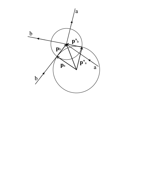
Figure 6: Head on collision of two particles. Conservation of 2D optical space momentum determines both particle speed after collision.

The length of the particles momenta stay unaltered by the collision; only their directions are changed. Fig. (6) exemplifies a collision situation. The addition of the momenta $\mathbf{p}_{a}+\mathbf{p}_{b}$ gives the total momentum that must stay unaltered by the collision. The length of individual momenta must also be preserved because the particles’ masses don’t change. The construction shows the only other way that two vectors of lengths $|\mathbf{p}_{a}|$ and $|\mathbf{p}_{b}|$ can be added so that their sum is preserved; these vectors are $\mathbf{p}^{\prime}_{a}$ and $\mathbf{p}^{\prime}_{b}$, respectively and their orientation gives the speed of both particles after the collision.

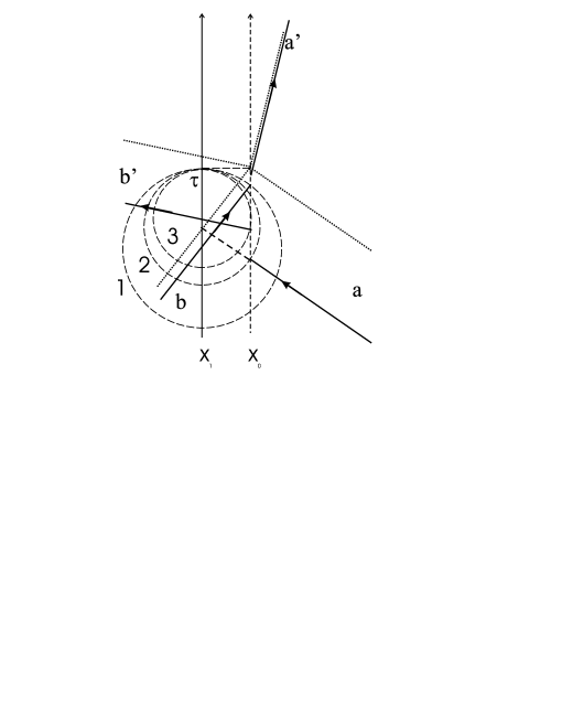
Figure 7: When represented on a distant observer’s frame the worldlines no longer intersect at the collision position.

The problem was analyzed from the point of view of an observer standing at the collision position. When represented on a distant observer’s frame, the particles’ worldlines no longer intersect at the collision position, as shown in Fig. 7 where $x_{0}$ and $x_{1}$ are the collision and observer’s positions, respectively. The collision instant $\tau$ is the time measured along each of the four different worldlines. The geometrical construction on the figure is such that circles 1, 2 and 3 have centers on the intersection of the observer’s worldline, at $x_{1}$ with the worldlines $b$, $a$ and $b^{\prime}$, respectively. The circle associated with $a^{\prime}$ worldline is not shown. All the circles cross $x_{1}$ at a common point $\tau$, ensuring that each circle’s radius is exactly the time that mediates between the instant of the associated worldline passing at $x_{1}$ and the collision instant. The point of intersection of each circle with the vertical line at $x_{0}$ marks the point of passage of the associated worldline by this position. The dotted lines meeting at $x_{0}$ represent the situation depicted on Fig. 6 and clearly highlight the difficulty in representing simultaneous events on distant observers’ frames.

8 Conclusions

4DO has been shown in previous work to be a viable alternative to general relativity, being able to produce identical predictions in most observable situations but offering reasonable explanations for phenomena that Einstein’s theory has not been able to accommodate comfortably. Furthermore, 4DO shows prospects of being compatible with standard theory, paving the ground for a unified theory of Physics, which has so far been the realm of string theory.

4DO is based on the use 4-dimensional movement space, resulting from the consideration of the usual 3-dimensional coordinates complemented by proper time. The physical meaning of this space is not intuitive and the present paper uses the established K-calculus to make a parallel derivation of special relativity and 4DO, allowing a real possibility of comparison between the two theories. The significance of the proper time coordinate is given special attention and its definition is made very clear in terms of just send and receive instants of radar pulses.

Special relativity and 4DO are also compared in terms of Lagrangian definition of worldlines and movement Hamiltonian. The final section of the paper discusses simultaneity through the solution of a two particle head-on collision problem. It is shown that a very simple graphical construction automatically solves energy and momentum conservation when the observer is located at the collision position. A further discussion of the representation for a distant observer further clarifies how simultaneity is accommodated by 4DO.

References

- [1] José B. Almeida. Optical interpretation of special relativity and quantum mechanics. In OSA Annual Meeting, Providence, RI, 2000. physics/0010076.
- [2] José B. Almeida. An alternative to Minkowski space-time. In GR 16, Durban, South Africa, 2001. gr-qc/0104029.
- [3] José B. Almeida. On the anomalies of gravity. gr-qc/0105036, 2001.
- [4] José B. Almeida. 4-dimensional optics, an alternative to relativity. gr-qc/0107083, 2001.
- [5] José B. Almeida. A theory of mass and gravity in 4-dimensional optics. physics/0109027, 2001.
- [6] Tom Van Flandern. The speed of gravity – what the experiments say. Phys. Lett. A, 250:1–11, 1998.
- [7] Brian Greene. The Elegant Universe: Superstrings, Hidden Dimensions, and the Quest for the Ultimate Theory. W. W. Norton & Company Inc., N. York, 1999.
- [8] Hermann Bondi. Relativity and Common Sense: A New Approach to Einstein. Dover pub., New York, 1980.
- [9] J. L. Martin. General Relativity: A Guide to its Consequences for Gravity and Cosmology. Ellis Horwood Ltd., U. K., 1988.
- [10] Ray D’Inverno. Introducing Einstein’s Relativity. Clarendon Press, Oxford, 1996.
- [11] Herbert Goldstein. Classical Mechanics. Addison Wesley, Reading, MA, 2nd. edition, 1980.