Passage of a Bessel Beam Through a Classically Forbidden Region

1 Introduction

The motion of an electromagnetic wave, through a classically-forbidden region, has recently attracted renewed interest because of its implication with regard to the theoretical and experimental problems of superluminality. From an experimental point of view, many papers provide an evidence of superluminality in different physical systems[1, 2, 3, 4, 5, 6]. Theoretically, the problem of a passage through a forbidden gap has been treated by considering plane waves at oblique incidence into a plane parallel layer of a medium with a refractive index smaller than the index of the surrounding medium, and also confined (Gaussian) beams, still at oblique incidence[7, 8, 9, 10]. In the present paper the case of a Bessel beam is examined, at normal incidence into the layer (Secs. II and III), in the scalar approximation (Sec. IV) and by developing also a vectorial treatment (Sec. V). Conclusions are reported in Sic. VI.

2 The Bessel beam

An interesting solution of the wave equation is represented by the Bessel beam with axial symmetry having, as known[11, 12], the following expression:

$$u(\rho,\>\psi,\>z)=AJ_{0}(k_{0}n\rho\sin\theta_{0})\exp(ik_{0}nz\cos\theta_{0})\>,$$ (1)

where $A$ is an amplitude factor, $J_{0}$ denotes the zero-order Bessel function of first kind, $\rho,\>\psi,\>z$ are cylindrical coordinates (Fig. 1a), $\theta_{0}$ is the parameter of the beam (Axicon angle), $n$ is the refractive index of the medium where the beam propagates, and $k_{0}$ is the wavenumber in the vacuum. The beam is independent of the angular coordinate $\psi$. The time factor $\exp(-i\omega t)$ is omitted in Eq. (1).

The unusual features of a Bessel beam are that its phase propagates (in the $z$ direction) with a velocity $v=c/(n\cos\theta_{0})$ larger than $c/n$[12, 13], and that it does not changes its shape during propagation (the amplitude is independent of $z$). The situation is similar to what occurs when only two plane waves interfere, the only difference being that the two-wave interference pattern occupies the whole space, while the field (1) is practically limited to a restricted zone of space $(k_{0}n\rho\sin\theta_{0}<2.4,\>2.4$ being the first zero of $J_{0}$). In this connection, it is worth noting that the field of Eq. (1) is not properly a beam, since it is not limited by a caustic surface, inasmuch as $J_{0}$ oscillates when its argument tends to infinity.

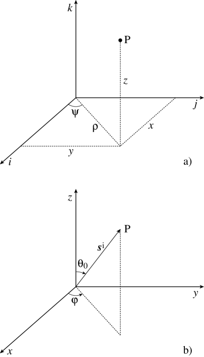
Figure 1: The coordinate systems

The meaning of the parameter $\theta_{0}$ is the following. Let us refer the space to a system of Cartesian coordinates $x,\>y,\>z$, (unit vectors i, j, k), such that

$$x = \rho\cos\psi$$

$$y = \rho\sin\psi$$

$$z = z$$ (2)

Let us also consider a system of spherical coordinates $r,\>\theta,\>\varphi$, with origin in the origin of the Cartesian coordinates, and the $\theta=0$ semiaxis coinciding with the positive $z$-axis.

Let us now consider a set of plane waves, with the same amplitude $Ad\varphi$, and with directions of propagation s = $\alpha$i+ $\beta$j + $\gamma$k making the same angle $\theta_{0}$ with the $z$-axis. Each wave can be written as

$$A\exp[ik_{0}n(\alpha x+\beta y+\gamma z)]\,d\varphi\>,$$ (3)

where the well-known relations hold (see Fig. 1b):

$$\alpha=\sin\theta_{0}\cos\varphi\,,\>\>\>\beta=\sin\theta_{0}\sin\varphi\,,\>\>\>\gamma=\cos\theta_{0}\,.$$ (4)

If we integrate expression (3) over $d\varphi$ between 0 and 2$\pi$, and recall the properties of the Bessel function $J_{0}$[14], we arrive at Eq. (1)

$$A \int_{0}^{2\pi}\,\exp[ik_{0}n(\alpha x+\beta y+\gamma z)]\,d\varphi$$

$$= A \,\exp(ik_{0}nz\cos\theta_{0})\int_{0}^{2\pi}\,\exp[ik_{0}n\rho(\cos\varphi\cos\psi+\sin\varphi\sin\psi)\sin\theta_{0}]d\varphi$$

$$= A \,2\pi J_{0}(k_{0}n\rho\sin\theta_{0})\exp(ik_{0}nz\cos\theta_{0})$$ (5)

If beam (1) impinges normally into a plane parallel layer of refractive index $n^{\prime}$, limited by the planes $z=0$ and $z=d$ (Fig.2), the plane waves (3) form an incidence angle $i=\theta_{0}$ which may be larger than the limit angle $i_{0}=\arcsin(n/n^{\prime})$. In this case, the plane waves undergo total reflection, and the layer is a classically-forbidden region for the Bessel beam, in spite of the fact that the beam impinges normally into the layer.

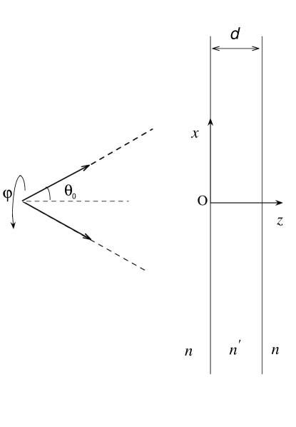
Figure 2: The layer and the impinging Bessel beam characterised by the Axicon angle $\theta_{0}$.

3 Total reflection for a Bessel beam

The preceding expansion of a Bessel beam in plane waves whose directions of propagation cover a conical surface of semiaperture $\theta_{0}$ immediately indicates what happens when the Bessel beam impinges (at $z=0$) into a plane surface separating two media of different refractive indexes $n$ and $n^{\prime}$. Each plane wave forms the same incidence angle $\theta_{0}$ and, hence, also the same refraction angle $\theta^{\prime}$, satisfying

$$n^{\prime}\sin\theta^{\prime}=n\sin\theta_{0}\,.$$ (6)

The refracted waves have the same amplitude, therefore, their superposition $u$ is a Bessel beam with parameter $\theta^{\prime}$:

$$u(\rho,\psi,z)=A^{\prime}J_{0}(k_{0}n^{\prime}\rho\sin\theta^{\prime})\exp(ik_{0}n^{\prime}z\cos\theta^{\prime})$$ (7)

Here, it may be interesting to note that, if $\cos\theta^{\prime}$ is real, the phase of the Bessel beam for $z>0$ propagates in the $z$-direction, normally therefore to the boundary. The phase velocity turns out to be $c/(n^{\prime}\cos\theta^{\prime})$, i.e. larger than the light velocity in the $n^{\prime}$ medium. If $\cos\theta^{\prime}$ is purely imaginary (that is, for $\theta_{0}$ larger than $i_{0}$), the single plane waves composing the incident Bessel beam are in total reflection, and therefore give rise to plane refracted waves the phase of which propagates parallel to the boundary. However, for the refracted Bessel beam, there is no phase propagation for $z>0$: there is a sort of stationary field. Here as follows, only the latter case will be considered, namely:

$$\sin\theta^{\prime}=\,\frac{n}{n^{\prime}}\,\sin\theta_{0}>1$$ (8)

with the notation

$$\cos\theta^{\prime}=i\Gamma,\>\>\>\>\>\>\>\>\>(\Gamma>0)\,.$$ (9)

4 The tunneling effect in the scalar approximation

If the beam of Eq. (1) impinges normally into the layer of Fig. 2, it gives rise:
i - on the left of the first boundary ($z<0$), to a reflected Bessel beam which propagates in the negative direction of the z-axis;
ii - inside the layer ($0<z<d$), to two Bessel beams, a “progressive” one and a “regressive” one;
iii - on the right of the second boundary ($z>d$), to one transmitted Bessel beam, which propagates in the positive $z$-direction.

The continuity conditions of the total field at the boundaries $z=0$ and $z=d$ may be easily satisfied with a suitable choice of the complex amplitudes of the beams, and of the parameter $\theta^{\prime}$ in the argument of the Bessel beams inside the layer. Using standard procedure, let us write the incident field in the form

$$u^{i}(\rho,\psi,z)=A^{i}\,2\pi J_{0}(k_{0}n\rho\sin\theta_{0})\exp(ik_{0}nz\cos\theta_{0})\>\>\>\>\>(z\leq 0)$$ (10)

the reflected field in the form

$$u^{r}(\rho,\psi,z)=A^{r}\,2\pi J_{0}(k_{0}n\rho\sin\theta_{0})\exp(-ik_{0}nz\cos\theta_{0})\>\>\>\>\>\>\>(z\leq 0)$$ (11)

the transmitted field in the form

$$u^{t}(\rho,\psi,z)=A^{t}\,2\pi J_{0}(k_{0}n\rho\sin\theta_{0})\exp(ik_{0}n(z-d)\cos\theta_{0})\>\>\>\>\>(z\geq d)$$ (12)

and, lastly, the progressive and regressive fields, respectively, in the forms

$$u^{+}(\rho,\psi,z) = A^{+}\,2\pi J_{0}(k_{0}n^{\prime}\rho\sin\theta^{\prime})\exp(-k_{0}n^{\prime}z\Gamma)$$

$$u^{-}(\rho,\psi,z) = A^{-}\,2\pi J_{0}(k_{0}n^{\prime}\rho\sin\theta^{\prime})\exp(k_{0}n^{\prime}z\Gamma)\,\>\>\>\>\>\>\>\>\>(0\leq z\leq d).$$ (13)

Due to the exponential dependence of $u^{+}$ and $u^{-}$ on $z$, the progressive and regressive beams inside the layer may be denoted as “evanescent” Bessel beams.

The ratio $R=A^{r}/A^{i}$ is the reflection coefficient of the layer for the Bessel beam; the ratio $T=A^{t}/A^{i}$ is the transmission coefficient.

By denoting the total field at any point of the space by $u^{tot}$, the boundary conditions can be written as

$$u^{tot}(z=0-)=u^{tot}(z=0+)$$

$$u^{tot}(z=d-0)=u^{tot}(z=d+0)$$ (14)

and

$$\frac{\partial}{\partial z}\,u^{tot}(z=0-)=\frac{\partial}{\partial z}\,u^{tot}(z=0+)$$

$$\frac{\partial}{\partial z}\,u^{tot}(z=d-0)=\frac{\partial}{\partial z}\,u^{tot}(z=d+0)$$ (15)

Upon the introduction of Eqs. (10) to (13) into Eqs. (14) and (15), the following conditions are found:

$$A^{i}+A^{r} = A^{+}+A^{-}$$

$$(A^{i}-A^{r})n\cos\theta_{0} = in^{\prime}\,\Gamma(A^{+}-A^{-})$$

$$A^{+}e_{1}+A^{-}e_{2} = A^{t}$$

$$in^{\prime}\,\Gamma(A^{+}e_{1}-A^{-}e_{2}) = A^{t}n\cos\theta_{0}\,,$$ (16)

where $e_{1}=\exp(-k_{0}n^{\prime}d\Gamma),\>e_{2}=1/e_{1}$.

The solution of system (16) is easily found and we have

$$\frac{A^{+}}{A^{i}}\,=\,\frac{e_{2}}{2n^{\prime}\,\Gamma}(n^{\prime}\Gamma-in\cos\theta_{0})T$$

$$\frac{A^{-}}{A^{i}}\,=\,\frac{e_{1}}{2n^{\prime}\,\Gamma}(n^{\prime}\Gamma+in\cos\theta_{0})T$$

$$\frac{A^{t}}{A^{i}}\,=T=\,\frac{4inn^{\prime}\Gamma\cos\theta_{0}}{e_{2}(n\cos\theta_{0}+in^{\prime}\Gamma)^{2}-e_{1}(n\cos\theta_{0}-in^{\prime}\Gamma)^{2}}$$ (17)

From the point of view of the field iside to the forbidden region, it should be noted that $A^{+}$ and $A^{-}$ are complex quantities that depend on $k_{0}$ and on the geometric characteristics of the system. If we denote the argument of $T$ by $\Phi_{T}$, and if we introduce a quantity $\Phi^{\prime}$ such that

$$\tan\Phi^{\prime}=\,\frac{n\cos\theta_{0}}{n^{\prime}\Gamma}$$ (18)

we can write

$$A^{+}=|A^{+}|\exp[i(\Phi_{T}-\Phi^{\prime})]$$

$$A^{-}=|A^{-}|\exp[i(\Phi_{T}+\Phi^{\prime})]\,.$$ (19)

Accordingly, the internal total field can be written as

$$u^{tot} = u^{+}+u^{-}=2\pi\,\exp(i\Phi_{T})J_{0}(k_{0}n\rho\sin\theta_{0})\times$$ (20)

$$\times \left[|A^{+}|\exp(-k_{0}n^{\prime}z\Gamma)\exp(-i\Phi^{\prime})+|A^{-}|\exp(k_{0}n^{\prime}z\Gamma)\exp(i\Phi^{\prime})\right]\,,$$

which shows that, inside the forbidden layer, the total field has a phase $\Phi=\Phi_{T}+\eta(z)$, with $\eta(z)$ such that

$$\tan\eta(z) = \,\frac{|A^{-}|\exp(k_{0}n^{\prime}z\Gamma)-|A^{+}|\exp(-k_{0}n^{\prime}z\Gamma)}{|A^{-}|\exp(k_{0}n^{\prime}z\Gamma)+|A^{+}|\exp(-k_{0}n^{\prime}z\Gamma)}\tan\Phi^{\prime}$$ (21)

$$= -\tanh[k_{0}n^{\prime}\Gamma(d-z)]\tan\Phi^{\prime}\,,$$

which propagates in the direction of the positive $z$-axis.

Equation (21) may be used to evaluate $|{\rm grad}\eta|=\partial\eta/\partial z$, the wavelength $\lambda^{\prime}=\lambda^{\prime}(z)$ and the phase velocity $v^{\prime}=v^{\prime}(z)$:

$$|{\rm grad}\eta| = \frac{k_{0}n\cos\theta_{0}\,\cos^{2}[\eta(z)]}{\cosh^{2}[k_{0}n^{\prime}\Gamma(d-z)]}$$

$$\lambda^{\prime} = \frac{2\pi}{|{\rm grad}\eta|}=\frac{\lambda_{0}}{n\cos\theta_{0}}\,\frac{\cosh^{2}[k_{0}n^{\prime}\Gamma(d-z)]}{\cos^{2}[\eta(z)]}$$

$$v^{\prime} = \frac{\omega}{|{\rm grad}\eta|}=\frac{c}{n\cos\theta_{0}}\,\frac{\cosh^{2}[k_{0}n^{\prime}\Gamma(d-z)]}{\cos^{2}[\eta(z)]}\,,$$ (22)

where $\lambda_{0}=2\pi/k_{0}$ denotes the free space plane-wave wavelength. It is interesting to note that for $z\rightarrow d,\>v^{\prime}\rightarrow c/(n\cos\theta_{0})$, which is equal to the phase velocity of the trasmitted ($z>d$) and incident ($z<0$) fields. This is a phenomenon similar to the one reported in Ref.[10].

The phase difference $\Delta\Phi$ of the total internal field at $z=d$ from $z=0$ is given by

$$\Delta\Phi=\arctan[\tanh(k_{0}n^{\prime}\Gamma d)\tan\Phi^{\prime}]\,,$$ (23)

while, as to the transmitted field, it can be noted (see Eq. (12)) that its phase at $z=d$ is

$$\Phi_{T}=\arctan\left[\frac{n^{2}\cos^{2}\theta_{0}-{n^{\prime}}^{2}\Gamma^{2}}{2nn^{\prime}\Gamma\cos\theta_{0}}\tanh(k_{0}n^{\prime}\Gamma d)\right]\,.$$ (24)

Thus, $\Phi_{T}$ is equal to the phase shift of the transmitted beam at $z=d$ with respect to that of the incident field at $z=0$. By comparing Eqs. (23) and (24), it appears that $\Phi_{T}$ does not coincide with the phase gained by the internal field in passing from $z=0$ to $z=d$.

5 The vectorial treatment

In this Section we use the vectorial algorithm for analysing the propagation of Bessel beams.

5.1 Quasi-TE and quasi-TM beams

For a vectorial treatment of the propagation of a Bessel beam it is sufficient to consider, for example, the function of Eq. (1) as the tangential component of the electric field E. Then, the Maxwell equations allow us to determine the longitudinal component of E, and the magnetic field H as well. The longitudinal component of E turns out to vanish on the $z$-axis, for $\rho=0$, where the tangential component has its maximum. Thus, such field (E, H) may be named quasi-TE. If the field (E, H) impinges normally on the layer of Fig. 2, it gives rise, as in the scalar approximation, to a reflected Bessel beam for $z<0$, to a transmitted beam for $z>d$, and to a progressive and a regressive Bessel beams for $0<z<d$. The progressive and regressive beams are evanescent if Eq. (8) holds.

Analogously, we can consider the function $u$ of Eq. (1) as the tangential component of a magnetic field H’, then from the Maxwell equations we can derive the longitudinal component of H’ and the associated electric field E’. The field (E’, H’) may be named quasi-TM.

The complex amplitudes of all the above beams may be determined by imposing, at the two boundaries, the continuity conditions for the tangential component of both the total electric and magnetic fields. This allows to determine in both cases the total field inside the forbidden region, its wavelength and its phase velocity.

Since the treatment is a little cumbersome, we report that different wavelength and different phase velocity are found for the quasi-TE and quasi-TM cases; here we limit ourselves to develop the simpler analysis in the TE and TM cases. To this end, let us consider a plane TE and a plane TM waves with a direction of propagation sⁱ = $\alpha$i + $\beta$j + $\gamma$k = $\sin\theta_{0}\cos\varphi$i + $\sin\theta_{0}\sin\varphi$j + $\cos\theta_{0}$k. Let them reflect and refract through the first boundary, then reflect and refract at the second boundary. Lastly, we integrate the three Cartesian components with respect to $\varphi$ between 0 and $2\pi$.

5.2 The TE case

This case has already been treated in Ref.[9, 10], but in the particular case of $\varphi=0$. Here, we have to generalise the results obtained therein.

For the incident field E${}^{i}=E_{x}$i $+E_{y}$j $(E_{z}=0)$, let us put

$$E_{x} = A_{x}\exp[\,ik_{0}n(x\sin\theta_{0}\cos\varphi+y\sin\theta_{0}\sin\varphi+z\cos\theta_{0})\,]d\varphi$$

$$E_{y} = A_{y}\exp[\,ik_{0}n(x\sin\theta_{0}\cos\varphi+y\sin\theta_{0}\sin\varphi+z\cos\theta_{0})\,]d\varphi\,.$$ (25)

Since Eⁱ is normal to sⁱ, the following relation must hold:

$$A_{x}\alpha+A_{y}\beta=0\>.$$

Hence,

$$A_{x}\cos\varphi+A_{y}\sin\varphi=0\,.$$ (26)

Equation (26) shows that $A_{x}$ and $A_{y}$ depend on $\varphi$. The solution of Eq. (26), which remains finite for any value of $\varphi$, is

$$A_{x} = A\sin\varphi$$

$$A_{y} = -A\cos\varphi\,,$$ (27)

where $A$ is a constant.

At this point, insertion of Eqs. (27) into Eqs. (25) and integration with respect to $\varphi$ yields (by putting $a=2\pi A$)

$$E_{x,beam} = i\,a\sin\psi J_{1}(k_{0}n\rho\sin\theta_{0})\exp\left(ik_{0}nz\cos\theta_{0}\right)$$

$$E_{y,beam} = -i\,a\cos\psi J_{1}(k_{0}n\rho\sin\theta_{0})\exp\left(ik_{0}nz\cos\theta_{0}\right)\,,$$ (28)

where $J_{1}$ is the Bessel function of the first order.

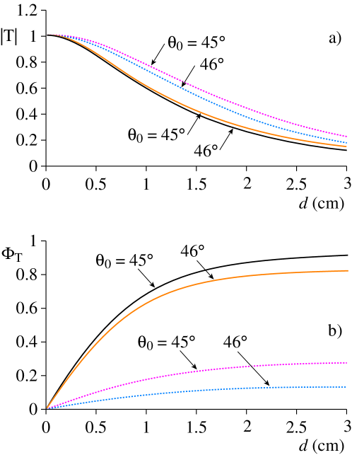
Figure 3: Amplitude (a) and phase (b) of the transmission coefficients $T$ in the TE case (solid lines) and in the TM case (dotted lines) plotted vs $d$ for two values of the parameter $\theta_{0}$. Other parameter values are: $\omega=60,\>n=1.5,\>n^{\prime}=1$.

The magnetic field H${}^{i}=H_{x}$i + $H_{y}$j + $H_{z}$k related to the Eⁱ field of the plane wave is found to be

$$H_{x} = \frac{A}{Z}\,\cos\theta_{0}\cos\varphi\exp[\,ik_{0}n(x\sin\theta_{0}\cos\varphi+y\sin\theta_{0}\sin\varphi+z\cos\theta_{0})\,]d\varphi$$

$$H_{y} = \frac{A}{Z}\cos\theta_{0}\sin\varphi\exp[\,ik_{0}n(x\sin\theta_{0}\cos\varphi+y\sin\theta_{0}\sin\varphi+z\cos\theta_{0})\,]d\varphi$$

$$H_{z} = -\,\frac{A}{Z}\sin\theta_{0}\exp[\,ik_{0}n(x\sin\theta_{0}\cos\varphi+y\sin\theta_{0}\sin\varphi+z\cos\theta_{0})\,]d\varphi\,,$$ (29)

where $Z=Z_{0}/n$, and $Z_{0}$ is the free space impedance. Hence, upon integration over $\varphi$, we obtain

$$H_{x,beam} = \frac{i\,a}{Z}\cos\theta_{0}\cos\psi J_{1}(k_{0}n\rho\sin\theta_{0})\exp\left(ik_{0}nz\cos\theta_{0}\right)$$

$$H_{y,beam} = \frac{i\,a}{Z}\cos\theta_{0}\sin\psi J_{1}(k_{0}n\rho\sin\theta_{0})\exp\left(ik_{0}nz\cos\theta_{0}\right)$$

$$H_{z,beam} = -\,\frac{a}{Z}\sin\theta_{0}J_{0}(k_{0}n\rho\sin\theta_{0})\exp\left(ik_{0}nz\cos\theta_{0}\right)\,.$$ (30)

A field described by Eqs. (28) and (30) can be denoted as a Bessel beam (of the first order), and has properties very similar to those of the Bessel beam of Eq. (1). However, only the longitudinal component of the magnetic field is of the type of Eq. (1), that is, picked on the axis at $\rho=0$; all other components for $\rho=0$ vanish. A TE plane wave like the one described above gives rise, at the incidence on the layer of Fig. 2, to a reflected first-order Bessel beam and to two transmitted “evanescent” Bessel beams. One of these is progressive and the other regressive, with coefficients $A^{+}$ and $A^{-}$ given by the first two Eqs. (17). At the second boundary of the layer, a transmitted first-order Bessel beam originates, with amplitude $A^{t}$ given by the third Eq. (17). Accordingly, the wavelength $\lambda_{TE}$ and the phase velocity $v_{TE}$ inside the layer are again given by Eqs. (22).

5.3 The TM case

The TM case may be treated in a way analogous to that of the TE case, arriving at similar results. The only difference lies in the fact that $n$ must be replaced by $n^{\prime}$, and vice versa, in the coefficients of system (16) (not in the propagation factors $e_{1}$ and $e_{2}$), analogously to what happens in the Fresnel formulas for the reflection and transmission coefficients of a real plane wave at a plane interface. Accordingly, the expression of $A^{+},\>A^{-},\>A^{t}$ and $\Phi^{\prime}$ must be replaced by

$$\left(\frac{A^{+}}{A^{i}}\right)_{TM}\, = \,\frac{e_{2}}{2n\Gamma}(n\Gamma-in^{\prime}\cos\theta_{0})$$

$$\left(\frac{A^{-}}{A^{i}}\right)_{TM}\, = \,\frac{e_{1}}{2n\Gamma}(n\Gamma+in^{\prime}\cos\theta_{0})$$

$$\left(\frac{A^{t}}{A^{i}}\right)_{TM}\, = T_{TM}=\,\frac{4inn^{\prime}\Gamma\cos\theta_{0}}{e_{2}(n^{\prime}\cos\theta_{0}+in\Gamma)^{2}-e_{1}(n^{\prime}\cos\theta_{0}-in\Gamma)^{2}}$$

$$\tan\Phi^{\prime\prime} = \,\frac{n^{\prime}\cos\theta_{0}}{n\Gamma}\,.$$ (31)

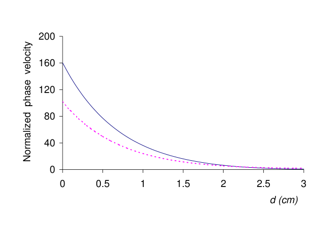
Figure 4: Normalised velocities $v_{TE}/c$ (solid line) and $v_{TM}/c$ (dotted line), as a function of $d$, for the same parameters values as in Fig. 3 and for $\theta_{0}=45^{\circ}$.

6 Conclusions

On the basis of the vectorial treatment we are now able to compare the TE and TM cases. In particular we can conclude that:

1 - The phase shift $\Delta\Phi$ of the transmitted TM beam (Eq. (23) with $\Phi^{\prime\prime}$ instead of $\Phi^{\prime}$) at $z=d$ with respect to the incident beam at $z=0$ is different from that of the TE case.

2 - The transmission coefficient $T$ for the TM case is different in amplitude (Fig. 3a) and phase (Fig. 3b) with respect to that of the TE case. Consequently, an incident Bessel beam formed by a TE component and by a TM component gives rise to a transmitted Bessel beam with a different polarisation.

We note that the amplitudes are slowly varying functions of $\theta_{0}$, for both TE and TM cases. On the contrary, the phase in the case of TE differs greatly with respect to the TM case, and both of them greatly vary with $\theta_{0}$.

3 - The phase velocity $v_{TM}$ and the wavelength $\lambda_{TM}$ inside the layer in the TM case are different from those of the TE case,

$$\lambda_{TM} = \frac{n\lambda_{0}}{{n^{\prime}}^{2}\cos\theta_{0}}\frac{\cosh^{2}[k_{0}n^{\prime}\Gamma(d-z)]}{\cos^{2}[\eta_{TM}(z)]}$$

$$v_{TM} = \frac{nc}{{n^{\prime}}^{2}\cos\theta_{0}}\frac{\cosh^{2}[k_{0}n^{\prime}\Gamma(d-z)]}{\cos^{2}[\eta_{TM}(z)]}$$ (32)

where $\eta_{TM}(z)$ is such that $\tan[\eta_{TM}(z)]=-\tanh[k_{0}n^{\prime}\Gamma(d-z)]\tan\Phi^{\prime\prime}$. Figure 4 shows the normalised phase velocities $v_{TM}/c$ (which is equal to $\lambda_{TM}/\lambda_{0}$) and $v_{TE}/c$ (equal to $\lambda_{TE}/\lambda_{0}$). We note that, immediately after the first boundary the motion is extremely fast since the effect of the second boundary, which originates the regressive (or “anti-evanescent”) beam, is negligible. We wish to recall that, in the absence of the second boundary, the phase velocity is infinite.

References

- [1] A. Ranfagni, D. Mugnai, P. Fabeni, G.P. Pazzi, Physica Scripta 42(1990) 508; Appl. Phys. Lett. 58 (1991) 774.
- [2] A. Enders, G. Nimtz, J. Phys. I (France) 2 (1992) 1693.
- [3] D. Mugnai, A. Ranfagni, L. S. Schulman, Phys. Rev. E 55 (1997) 3593.
- [4] D. Mugnai, A. Ranfagni, L. Ronchi, Phys. Lett. A 247, (1998) 281.
- [5] A.M. Steinberg, P.G. Kwiat, R.Y. Chiao, Phys. Rev. Lett. 71 (1993)708.
- [6] Ph. Balcou, L. Dutriaux, Phys. Rev. Lett. 78, 851 (1997).
- [7] S. Bosanac, Phys. Rev. A 28 (1983) 577.
- [8] A. M. Steinberg and R. Y. Chiao, Phys. Rev. A 49 (1994) 3283.
- [9] D. Mugnai, A. Ranfagni, L. Ronchi, Atti della Fondazione G. Ronchi 1 (1998) 777.
- [10] D. Mugnai, Optics Commun. 175(2000) 309.
- [11] J. Durnin, J.J. Miceli Jr., J.H. Eberly, Phys. Rev. Lett. 58 (1987) 1499.
- [12] P. Saari, K. Reivelt, Phys. Rev. Lett. 79(1997) 4135.
- [13] D. Mugnai, A. Ranfagni, R. Ruggeri, Phys. Rev. Lett. 84 (2000) 4830.
- [14] G.N. Watson, Theory of Bessel Functions, Cambridge, 1922.