[

DSF$-$23/2001

Majorana solution of the Thomas-Fermi equation

Abstract

We report on an original method, due to Majorana, leading to a semi-analytical series solution of the Thomas-Fermi equation, with appropriate boundary conditions, in terms of only one quadrature. We also deduce a general formula for such a solution which avoids numerical integration, but is expressed in terms of the roots of a given polynomial equation.

PACS numbers: 31.15.Bs, 31.15.-p, 02.70.-c

] In 1928 Majorana found an interesting semi-analytical solution of the Thomas-Fermi equation [1] which, unfortunately, remained unpublished and unknown until now (see [2]). We set forth here a concise study of such a solution in view of its potential relevance in atomic physics as well as in nuclear physics (as, for example, in some questions related to nuclear matter in neutron stars [3]).
The problem is to find the Thomas-Fermi function $\varphi(x)$ obeying the differential equation:

$$\varphi^{\prime\prime}\;=\;\frac{\varphi^{3/2}}{\sqrt{x}}$$ (1)

with the boundary conditions:

$$\varphi(0) = 1$$ (2)

$$\varphi(\infty) = 0~{}~{}~{}.$$ (3)

An exact particular solution of Eq. (1) satisfying, however, only the condition (3), was discovered by Sommerfeld [4]:

$$\varphi\;=\;\frac{144}{x^{3}}~{}~{}~{}.$$ (4)

This can be regarded as an asymptotic expansion of the desired solution, and Sommerfeld himself considered a “correction” (in some sense) to Eq. (4) in such a way to take into account the condition (3). However, this “corrected” approximate solution had a divergent first derivative for $x=0$ [4].
As will be clear below, Majorana solution can be considered as a modification of Eq. (4) as well, but the method followed by him is extremely original and very different from the one used by Sommerfeld.
Let us consider solutions of the Thomas-Fermi equation (1) which are expressed in parametric form:

$$\begin{array}[]{rcl}\displaystyle x&=&\displaystyle x(t)\\ &&\\ \displaystyle\varphi&=&\displaystyle\varphi(t)~{}~{}~{}.\end{array}$$ (5)

To be definite, throughout this paper we will use a prime ^′ or a dot $\dot{}$ to denote derivatives with respect to $x$ or $t$, respectively. The strategy adopted by Majorana is to perform a double change of variables:

$$x~{},~{}\varphi(x)~{}~{}~{}~{}~{}\longrightarrow~{}~{}~{}~{}~{}t~{},~{}u(t)$$ (6)

where the novel unknown function is $u(t)$. The relation connecting the two sets of variables (assumed to be invertible) has a differential nature, that is:

$$\begin{array}[]{rcl}t&=&t(x,\varphi)\\ &&\\ u&=&u(\varphi,\varphi^{\prime})~{}~{}~{}.\end{array}$$ (7)

In such a way the second order differential equation (1) for $\varphi$ is transformed into a first order equation for $u$. Note, however, that in general Eqs. (7) are implicit equations for $t$ and $u$, since $x$ and $\varphi$ depend on them (one is looking for parametric solutions in terms of the parameter $t$ and the unknown function $u$). For the specific case of the Thomas-Fermi equation, Majorana introduced the following transformation:

$$t = 144^{-1/6}\,x^{1/2}\,\varphi^{1/6}$$ (8)

$$u = -\,\left(\frac{16}{3}\right)^{1/3}\,\varphi^{-4/3}\,\varphi^{\prime}~{}~{}~{}.$$ (9)

Observe that Eq. (8) is reminiscent of the Sommerfeld solution, since it can be cast into the form:

$$\varphi\;=\;\frac{144}{x^{3}}\,t^{6}~{}~{}~{}.$$ (10)

The differential equation for $u(t)$ is obtained by taking the $t-$derivative of Eq. (9):

$$\frac{du}{dt}\;=\;-\,\left(\frac{16}{3}\right)^{1/3}\,\dot{x}\,\varphi^{-4/3}\,\left[-\,\frac{4}{3}\,\frac{\varphi^{\prime 2}}{\varphi}\,+\,\varphi^{\prime\prime}\right]$$ (11)

and inserting Eq. (1):

$$\frac{du}{dt}\;=\;-\,\left(\frac{16}{3}\right)^{1/3}\,\dot{x}\,\varphi^{-4/3}\,\left[-\,\frac{4}{3}\,\frac{\varphi^{\prime 2}}{\varphi}\,+\,\frac{\varphi^{3/2}}{x^{1/2}}\right]~{}~{}~{}.$$ (12)

By using Eq. (8) and Eq. (9) to eliminate $x^{1/2}$ and $\varphi^{\prime 2}$, respectively, we obtain:

$$\frac{du}{dt}\;=\;\left(\frac{4}{9}\right)^{1/3}\,\frac{tu^{2}-1}{t}\,\dot{x}\,\varphi^{1/3}~{}~{}~{}.$$ (13)

We have now to express the quantity $\dot{x}\varphi^{1/3}$ in terms of $t,u$. From Eq. (8),

$$x\;=\;144^{1/3}\,t^{2}\,\varphi^{1/3}~{}~{}~{},$$ (14)

by taking the explicit $t-$derivative of both sides,

$$\dot{x}\;=\;144^{1/3}\,\left[2t\,\varphi^{-1/3}\,+\,t^{2}\,\dot{x}\,\left(-\,\frac{1}{3}\,\varphi^{-4/3}\,\varphi^{\prime}\right)\right]~{}~{}~{},$$ (15)

after some algebra we get:

$$\dot{x}\,\varphi^{1/3}\;=\;144^{1/3}\,\frac{2t}{1-t^{2}u}~{}~{}~{}.$$ (16)

By inserting this result into Eq. (13) we finally have the differential equation for $u(t)$:

$$\frac{du}{dt}\;=\;8\,\frac{tu^{2}-1}{1-t^{2}u}~{}~{}~{}.$$ (17)

The condition (2) implies, from Eqs. (8),(9), that $t=0$ for $x=0$ and:

$$u(0)\;=\;-\,\left(\frac{16}{3}\right)^{1/3}\,\varphi^{\prime}_{0}$$ (18)

where $\varphi^{\prime}_{0}=\varphi^{\prime}(x=0)$. The initial condition to be satisfied by $u(t)$ for the univocal solution of Eq. (17) is obtained from the boundary condition (3) by inserting the Sommerfeld asymptotic expansion (4) into Eqs. (8),(9). For $x\rightarrow\infty$ we have $t=1$ and

$$u(1)\;=\;1~{}~{}~{}.$$ (19)

We then easily recognize that the branch of $u(t)$ giving the Thomas-Fermi function (in parametric form) is the one between $t=0$ and $t=1$. In this interval we look for the solution of Eq. (17) by using a series expansion in powers of the variable $\tau=1-t$:

$$u\;=\;a_{0}\,+\,a_{1}\,\tau\,+\,a_{2}\,\tau^{2}\,+\,a_{3}\,\tau^{3}\,+\,\dots~{}~{}~{}.$$ (20)

From the condition (19) we immediately have:

$$a_{0}\;=\;1~{}~{}~{}.$$ (21)

The other coefficients are obtained by an iterative formula coming from the substitution of (20) into Eq. (17):

$$\sum_{k=0}^{\infty}\,\sum_{l=0}^{\infty}\,A(k,l)\,\tau^{k+l}\;=\;0$$ (22)

where:

$$A(k,l) = a_{k}\left[(l+1)a_{l+1}-2(l+4)a_{l}+(l+7)a_{l-1}\right]+$$ (23)

$$-\,(k+l+1)\delta_{l0}a_{k+l+1}+8\delta_{k0}\delta_{l0}$$ (24)

(we define $a_{-1}=0$). Eq. (22) can also be cast in the form ($k+l=m$, $l=n$):

$$\sum_{m=0}^{\infty}\,\left(\sum_{n=0}^{m}\,A(m-n,n)\right)\,\tau^{m}\;=\;0$$ (25)

so that, for fixed $m$, the relation determining the series coefficients is the following:

$$\sum_{n=0}^{m}\,a_{m-n}\left[(n+1)a_{n+1}-2(n+4)a_{n}+\right.$$ (26)

$$\left.+(n+7)(1-\delta_{n0})a_{n-1}\right]\;=\;(m+1)a_{m+1}-8\delta_{m0}$$ (27)

(we have explicitly used that $a_{-1}=0$), with $m=0,1,2,3,\dots$. The equation (27) for $m=0$:

$$\left(a_{0}-1\right)\,\left[a_{1}-8\left(a_{0}+1\right)\right]\;=\;0$$ (28)

is identically satisfied due to Eq. (21). For $m=1$ we have a second degree algebraic equation for $a_{1}$:

$$a_{1}^{2}\,-\,18\,a_{1}\,+\,8\;=\;0$$ (29)

of which we have to choose the smallest root (we are performing a perturbative expansion):

$$a_{1}\;=\;9-\sqrt{73}~{}~{}~{}.$$ (30)

The remaining coefficients are determined, using Eqs. (21) and (30), by linear relations. In fact excluding the cases with $m=0,1$, after some algebra Eq. (27) can be written as:

$$a_{m} = \frac{1}{2(m+8)-(m+1)a_{1}}\left\{\sum_{n=1}^{m-2}\,a_{m-n}\left[(n+1)a_{n+1}+\right.\right.$$ (31)

$$\left.-2(n+4)a_{n}+(n+7)a_{n-1}\right]+a_{m-1}\left[(m+7)+\right.$$ (32)

$$\left.\left.-2(m+3)a_{1}\right]+a_{m-2}\left[(m+6)a_{1}\right]\right\}~{}~{}~{}.$$ (33)

Note that the sum in the RHS involves coefficient $a_{i}$ with indices $i\leq m-1$, so that the relation in (33) gives explicitly the value of $a_{m}$ once the previous $m-1$ coefficients $a_{m-1},a_{m-2},\dots,a_{2},a_{1}$ (and $a_{0}$) are known.
The series expansion in (20) is uniformly convergent in the interval $[0,1]$ for $\tau$, since the series made of the coefficients only, $\sum_{n=0}^{\infty}\,a_{n}$, is convergent. In fact, by setting $\tau=1$ ($t=0$) into (20), from Eq. (18) we have:

$$-\,\varphi^{\prime}_{0}\;=\;\left(\frac{3}{16}\right)^{1/3}\,\sum_{n=0}^{\infty}\,a_{n}~{}~{}~{},$$ (34)

which shows that the sum of such a series is determined by the (finite) value of $\varphi^{\prime}_{0}$ ($\varphi^{\prime}_{0}\simeq 1.588$ and thus $\sum_{n=0}^{\infty}\,a_{n}\simeq 2.7746$). Note also that the coefficients $a_{n}$ are positive definite and that the series in (34) exhibits geometric convergence with $a_{n}/a_{n-1}\sim 4/5$ for $n\rightarrow\infty$. The numeric values of the first 20 coefficients are reported in Table I.

TABLE I.: Numerical values for the first 20 coefficients for the series expansion of the function $u(t)$ in Eq. (20).

$a_{1}$	0.455996	$a_{11}$	0.0316498
$a_{2}$	0.304455	$a_{12}$	0.0252839
$a_{3}$	0.222180	$a_{13}$	0.0202322
$a_{4}$	0.168213	$a_{14}$	0.0162136
$a_{5}$	0.129804	$a_{15}$	0.0130101
$a_{6}$	0.101300	$a_{16}$	0.0104518
$a_{7}$	0.0796352	$a_{17}$	0.00840559
$a_{8}$	0.0629230	$a_{18}$	0.00676661
$a_{9}$	0.0499053	$a_{19}$	0.00545216
$a_{10}$	0.0396962	$a_{20}$	0.00439678

Given the function $u(t)$ we have now to look for the parametric solution $x=x(t)$, $\varphi=\varphi(t)$ of the Thomas-Fermi equation. To this end let us put:

$$\varphi(t)\;=\;\exp\left\{\int_{0}^{t}\,w(t)\,dt\right\}$$ (35)

where $w(t)$ is an auxiliary function to be determined in terms of $u(t)$, and the condition (2) (or $\varphi(t=0)=1$) is automatically satisfied. By inserting Eq. (35) into Eq. (9) and using (16) we immediately find:

$$w\;=\;-\frac{6ut}{1-t^{2}u}~{}~{}~{}.$$ (36)

Summing up, the parametric solution of Eq. (1) with the boundary conditions (2), (3) takes the form:

$$\begin{array}[]{rcl}x(t)&=&\displaystyle\sqrt[3]{144}\,t^{2}\,e^{2{\cal I}(t)}\\ &&\\ \varphi(t)&=&\displaystyle e^{-6{\cal I}(t)}\end{array}$$ (37)

with:

$${\cal I}(t)\;=\;\int_{0}^{t}\,\frac{ut}{1-t^{2}u}\,dt$$ (38)

and $u(t)$ is given by the series expansion in (20) with the coefficients determined by (21), (30) and (33). Eq. (37) represents the celebrated Majorana solution of the Thomas-Fermi equation; it is given in terms of only one quadrature .
We have performed numerically the integration in (38) stopping the series expansion in (20) at the terms with $n=10$ and $n=20$, respectively, and compared the parametric solutions thus obtained from (37) with the exact (numerical) solution of the Thomas-Fermi equation. We found that the two Majorana solutions approximate (for excess) the exact solution with relative errors of the order of $0.1\%$ and $0.01\%$, respectively.
We can also obtain an approximate (by defect) analytic solution by inserting the series expansion (20) into the expression (38):

$${\cal I}(t) = \int_{1-t}^{1}\,\frac{u(1-\tau)}{1-(1-\tau)^{2}u}\,d\tau\;=$$ (39)

$$= \int_{1-t}^{1}\,\frac{1+b_{1}\tau+b_{2}\tau^{2}+\dots}{c_{1}\tau+c_{2}\tau^{2}+\dots}\,d\tau$$ (40)

with:

$$\begin{array}[]{rcl}b_{n}&=&a_{n}\,-\,a_{n-1}\\ &&\\ c_{n}&=&b_{n-1}\,-\,b_{n}\end{array}$$ (41)

for $n\geq 1$, while $b_{0}=1$ and $c_{0}=0$. Note that:

$$\begin{array}[]{rcl}b_{n}\,<\,0&{}{}{}{}{}{}\hfil&{\mathrm{f}or}~{}n\,\geq\,1\\ &&\\ c_{n}\,<\,0&{}{}{}{}{}{}\hfil&{\mathrm{f}or}~{}n\,>\,1\end{array}$$ (42)

(and $b_{0},c_{1}>0$). If we neglect $O(\tau^{2})$ terms in (40), the quantity ${\cal I}(t)$ is approximated by:

$${\cal I}(t)\;=\;\frac{b_{1}}{c_{1}}\,t\,-\,\frac{1}{c_{1}}\,\log\,(1-t)$$ (43)

and, in terms of the original $a_{n}$ coefficients, the approximate parametric solution of the Thomas-Fermi equation is:

$$\begin{array}[]{rcl}x(t)&=&\displaystyle\sqrt[3]{144}\,t^{2}\,(1-t)^{-\frac{2}{2-a_{1}}}\,e^{-2\frac{1-a_{1}}{2-a_{1}}t}\\ &&\\ \varphi(t)&=&\displaystyle(1-t)^{\frac{6}{2-a_{1}}}\,e^{6\frac{1-a_{1}}{2-a_{1}}t}~{}~{}~{}.\end{array}$$ (44)

In Fig. 1 we compare the above solution with the exact (numerical) one.

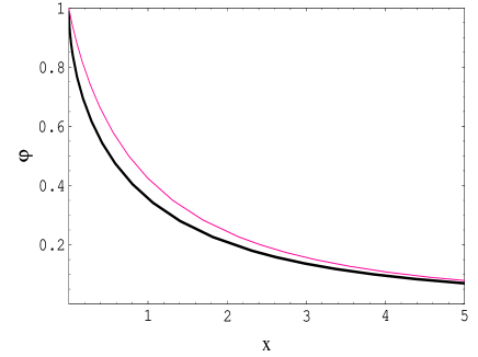
FIG. 1.: The Thomas-Fermi function $\varphi(x)$. The thin (upper) line refers to the exact (numerical) solution of Eq. (1), while the thick (lower) one corresponds to the parametric solution reported in Eqs. (44).

More in general, we can truncate the series in (40) to a certain power $\tau^{k}$ and thus the integrand function is approximated by a rational function:

$$F(\tau)\;\equiv\;\frac{1+b_{1}\tau+b_{2}\tau^{2}+\dots+b_{k}\tau^{k}}{c_{1}\tau+c_{2}\tau^{2}+\dots+c_{k}\tau_{k}}\;\equiv\;\frac{P(\tau)}{Q(\tau)}~{}~{}~{}.$$ (45)

Let us then assume that the roots $\tau_{i}$ ($i=1,2,\dots,k$) of the polynomial in the denominator,

$$Q(\tau_{i})\;=\;0~{}~{}~{},$$ (46)

are known, so that we can decompose the function $F(t)$ in a sum of simple rational functions :

$$\frac{1}{Q(\tau)}\;=\;\frac{1}{c_{k}}\,\left(\frac{f_{1}}{\tau-\tau_{1}}\,+\,\frac{f_{2}}{\tau-\tau_{2}}\,+\,\dots\,+\,\frac{f_{k}}{\tau-\tau_{k}}\right)$$ (47)

and:

$$F(\tau) = \frac{1}{c_{k}}\,\left(1\,+\,b_{1}\tau\,+\,b_{2}\tau^{2}\,+\,\dots\,+\,b_{k}\tau^{k}\right)\,{\cdot}$$ (48)

$${\cdot}\left(\frac{f_{1}}{\tau-\tau_{1}}\,+\,\frac{f_{2}}{\tau-\tau_{2}}\,+\,\dots\,+\,\frac{f_{k}}{\tau-\tau_{k}}\right)~{}~{}~{}.$$ (49)

The expressions for the coefficients $f_{i}$ ($i=1,2,\dots,k$) in terms of the roots $\tau_{i}$ are as follows:

$$f_{i}\;=\;\prod_{\begin{array}[]{c}l=1\\ l\neq i\end{array}}^{\displaystyle k}\,\frac{1}{\tau_{i}-\tau_{l}}~{}~{}~{}.$$ (50)

By inserting the decomposition (49) into Eq. (40), the integral ${\cal I}(t)$ is thus given by a (double) sum whose generic element has the following form:

$$\int_{1-t}^{1}\,\frac{\tau^{n}}{\tau-\tau_{i}}\,d\tau\;=\;-\tau_{i}^{n}\,\log\,\frac{1-\tau_{i}-t}{1-\tau_{i}}\,+$$ (51)

$$+\,\sum_{l=1}^{n}\,\left(\begin{array}[]{c}n\\ l\end{array}\right)\,\frac{\tau_{i}^{n-l}}{l}\,\left((1-\tau_{i})^{l}\,-\,(1-\tau_{i}-t)^{l}\right)~{}~{}~{}.$$ (54)

Then, in general, the parametric solution of Eq. (1) can be formally written as:

$$\begin{array}[]{rcl}x(t)&=&\displaystyle\sqrt[3]{144}\,t^{2}\,\epsilon^{2}(t)\\ &&\\ \varphi(t)&=&\displaystyle\epsilon^{-6}(t)\end{array}$$ (55)

where $\epsilon(t)=e^{{\cal I}(t)}$ is approximated by:

$$\epsilon(t)\;=\;\left[\prod_{i=1}^{k}\,\left(\frac{1-\tau_{i}-t}{1-\tau_{i}}\right)^{-\frac{1}{c_{k}}f_{i}\sum_{n=0}^{k}b_{n}\tau_{i}^{n}}\right]\,{\cdot}$$ (56)

$${\cdot}\,\left[\prod_{i=1}^{k}\,\prod_{n=1}^{k}\,\prod_{l=1}^{n}\,e^{-\frac{1}{c_{k}}f_{i}\left(\begin{array}[]{c}n\\ l\end{array}\right)\,\frac{b_{n}\tau_{i}^{n-l}}{l}\,\left((1-\tau_{i}-t)^{l}\,-\,(1-\tau_{i})^{l}\right)}\right]$$ (59)

Obviously, using the method described above, the exact result is recovered in the limit $k\rightarrow\infty$. This procedure can, however, be employed for getting approximate but accurate solutions of the Thomas-Fermi equation since, as it is clear from above, we have translated a numerical integration problem (see Eq. (38)) into the one of a numerical search for the roots of the polynomial $Q(\tau)$. Note also that we already know one of such roots (namely, $\tau_{1}=0$) given the particular form of $Q(\tau)$. This implies that, since the general solution of a fourth-degree polynomial equation in terms of radicals is known, from (55) and (56) we can get an analytic approximate solution by considering terms in the series in (40) up to order $O(\tau^{5})$, thus obtaining a certainly much better approximation to Eq. (37) than Eq. (44). We do not report here the explicit form of such a solution because of its very long expression.
Summarizing, in this paper we have reported on an original method, due to Majorana, forwarding a semi-analytical solution of the Thomas-Fermi equation (1) with boundary conditions (2), (3). The procedure applies as well to different boundary conditions, although the constraint (2) is always automatically satisfied. This corresponds to physical situations present in atomic as well as in nuclear physics. We have further studied the Majorana series solution thus obtaining a general formula whose degree of approximation is limited by the one for searching roots of a given polynomial rather than to the one for integrating a rational function.
The method used by Majorana for solving the Thomas-Fermi equation can be generalized in order to study a large class of ordinary differential equations, but this will be discussed elsewhere.

- [1] L.H. Thomas, Proc. Cambridge Phil. Soc., 23 (1924) 542; E. Fermi, Zeit. Phys. 48 (1928) 73.
- [2] S. Esposito, E. Majorana jr, A. van der Merwe and E. Recami, Ettore Majorana: notebooks in theoretical physics (Kluwer, New York, to appear during 2001).
- [3] S.L. Shapiro and S.A. Teukolsky, Black Holes, White Dwarfs and Neutron Stars (Wiley, New York, 1983).
- [4] A. Sommerfeld, Rend. R. Accademia dei Lincei, 15 (1932) 788.