Steep sharp-crested gravity waves on deep water

Abstract

A new type of steady steep two-dimensional irrotational symmetric periodic gravity waves on inviscid incompressible fluid of infinite depth is revealed. We demonstrate that these waves have sharper crests in comparison with the Stokes waves of the same wavelength and steepness. The speed of a fluid particle at the crest of new waves is greater than their phase speed.

A proper understanding of various wave phenomena on the ocean surface, such as modulation effects and instabilities of large amplitude wave trains Schwartz and Fenton (1982), McLean et al. (1981), formation of solitary Camassa and Holm (1993), freak Onorato et al. (2001), and breaking waves Banner and Peregrine (1993); Saffman and Yuen (1980), requires knowledge of a form and dynamics of steep water waves. For the first time surface waves of finite amplitude were considered by Stokes (1880). Stokes conjectured that such waves must have a maximal amplitude (the limiting wave) and suggested that a free surface of the limiting wave near the crest forms a sharp corner with the $120^{\circ}$ internal angle (the Stokes corner flow). A strict mathematical proof of the existence of small amplitude Stokes waves was given by Nekrasov. Toland (1978) proved that Nekrasov’s equation has a limiting solution describing a progressive periodic wave train which is such that the flow speed at the crest equals to the train phase speed, in a reference frame where fluid is motionless at infinite depth. Longuet-Higgins and Fox (1977) constructed asymptotic expansions for waves close to the $120^{\circ}$-cusped wave (almost highest waves) and showed that the wave profile oscillates infinitely as the limiting wave is approached. Later, in Longuet-Higgins et al. (1994), the crest of a steep, irrotational gravity wave was theoretically shown to be unstable.

The purpose of the present work is to give evidence that a second branch of two-dimensional irrotational symmetric periodic gravity waves of permanent form exists besides the Stokes waves of the same wavelength. The original motivation is as follows: the Bernoulli equation is quadratic in velocity and admits two values of the particle speed at the crest. The first one corresponds to the Stokes branch of symmetric waves for which the particle speed at the crest is smaller than the wave phase speed. The opposite inequality takes place for the second branch which might correspond to a new type of waves. In the second part of the Letter, we prove this numerically by using two different methods.

Consider a symmetric two-dimensional periodic train of waves which propagates without changing a form from left to right along the $x$-axis with the constant speed $c$ relative to the motionless fluid at infinite depth. The set of equations governing steady potential gravity waves on a surface of irrotational, inviscid, incompressible fluid is

$$\mathit{\Phi}_{xx}+\mathit{\Phi}_{yy}=0, -\infty<y<\eta(\theta);$$ (1)

$$\left(c-\mathit{\Phi}_{x}\right)^{2}+\mathit{\Phi}_{y}^{2}+2\eta=c^{2}, y=\eta(\theta);$$ (2)

$$\left(c-\mathit{\Phi}_{x}\right)\eta_{x}+\mathit{\Phi}_{y}=0, y=\eta(\theta);$$ (3)

$$\mathit{\Phi}_{x}=0,~{}\mathit{\Phi}_{y}=0,~{}y=-\infty; \theta=x-ct.$$ (4)

where $\mathit{\Phi}(\theta,~{}y)$ is the velocity potential, $\eta(\theta)$ is the elevation of a free surface, and $y$ is the upward vertical axis such that $y=0$ is the still water level. We have chosen the units of time and length such that the acceleration due to gravity and wavenumber are equal to unity.

As it follows from the Bernoulli equation (2), a solution may be not single-valued in the vicinity of the limiting point. Indeed, the particle speed at the crest $q(0)$ is horizontal and is defined as follows:

$$\mathit{\Phi}_{x}\left(0,~{}\eta(0)\right)=q(0)=c\pm\sqrt{c^{2}-2\eta(0)},$$ (5)

$\eta(0)$ being the height of the crest above the still water level. The “$-$” sign corresponds to the classical Stokes branch. The value $\eta_{\max}(0)=c^{2}/2$ corresponds to the Stokes wave of limiting amplitude. In this case, the particle speed at the crest is exactly equal to the wave phase speed: $q_{\max}(0)=c$. Taking into account both signs in expression (5), we assume that a second branch of solutions should exist apart from the Stokes waves, at $\eta(0)<\eta_{\max}(0)$. The particle speed at the crest of a new gravity wave must be greater than $c$ and has to increase from $c$ to $2c$ while the wave height decreases from $\eta_{\max}(0)$ to $0$. Moreover, the mean levels of these two flows relative to the level $y=0$ of still water must also be different:

$$\frac{1}{2\pi}\int_{0}^{2\pi}\eta^{(i)}(x)dx=\eta_{0}^{(i)},~{}~{}i=1,~{}2.$$ (6)

Thus, the existence of a second branch of solutions of the set of equations (1)-(4) does not contradict Garabedian’s theorem Garabedian (1965) that gravity waves are unique if all crests and all troughs are of the same height because the latter was proved for a flow with the same mean level.

To construct a numerical algorithm we use the method of the truncated Fourier series and the collocation method, in a plane of independent spatial variables.

The method of the Fourier approximations. Let us introduce the complex function $R(\theta,~{}y)$ such that

$$\mathit{\Phi}=-ic(R-R^{*}),~{}~{}\mathit{\Psi}=c(R+R^{*})$$ (7)

where $\mathit{\Psi}$ is the stream function, ^∗ is the complex conjugate. Using the relations $\mathit{\Phi}_{x}=\mathit{\Psi}_{y},~{}\mathit{\Phi}_{y}=-\mathit{\Psi}_{x}$, the kinematic boundary condition (3) can be presented as follows:

$$\frac{d}{dx}\bigl{(}R\left(\theta,~{}\eta\right)+R^{*}\left(\theta,~{}\eta\right)-\eta(\theta)\bigr{)}=0.$$ (8)

Approximate symmetric stationary solutions of Eq. (1, 2, 8, 4) are looked for in the form of the truncated Fourier series with real coefficients

$$R(\theta,~{}y) = \sum_{n=1}^{N}\xi_{n}\exp\bigl{(}n(y+i\theta)\bigr{)};$$ (9)

$$\eta(\theta) = \sum_{n=-M}^{M}\eta_{n}\exp(in\theta),~{}\eta_{-n}=\eta_{n};$$ (10)

where the Fourier harmonics $\xi_{n},~{}\eta_{n}$, and the wave speed $c$ are functions of the wave steepness $A$ determined by the peak-to-trough height:

$$A=\frac{\eta(0)-\eta(\pi)}{2\pi}=\frac{2}{\pi}\sum_{n=0}^{[M/2]}\eta_{2n+1},$$ (11)

square brackets designate the integer part. Substitution of expansions (9) and (10) into the dynamical and kinematic boundary conditions (2), (8) (the Laplace equation (1) and boundary condition (4) are satisfied exactly) yields the set of $N+M+1$ non-linear algebraic equations for the harmonics $\xi_{n},~{}\eta_{n}$, and the wave speed $c$

$$\sum_{n_{1}=1}^{N}\xi_{n_{1}}\bigl{(}f_{n-n_{1}}^{n_{1}}+f_{n+n_{1}}^{n_{1}}\bigr{)} = \eta_{n},~{}n=\overline{1,~{}N};$$ (12)

$$c^{2}\sum_{n_{1}=1}^{N}n_{1}\xi_{n_{1}}\bigl{(}f_{n-n_{1}}^{n_{1}}+f_{n+n_{1}}^{n_{1}}$$

$$-2\sum_{n_{2}=1}^{N}n_{2}\xi_{n_{2}}f_{n+n_{1}-n_{2}}^{n_{1}+n_{2}}\bigr{)} = \eta_{n},~{}n=\overline{0,~{}M};$$ (13)

where $f_{n}^{n_{1}}$ are the Fourier harmonics of the exponential functions $\exp(n_{1}\eta(\theta))$:

$$f_{n}^{n_{1}}=\frac{1}{2\pi}\int_{0}^{2\pi}\exp\bigl{(}n_{1}\eta(\theta)-in\theta\bigr{)}d\theta,~{}~{}f_{-n}^{n_{1}}=f_{n}^{n_{1}}.$$ (14)

They were being calculated using the fast Fourier transform (FFT). In addition to these equations, the connection (11) between the harmonics $\eta_{n}$ and the wave steepness $A$ should be taken into account.

The set of equations (12), (13) was being solved by Newton’s iterations in arbitrary precision computer arithmetic. Since the non-linearity over $\xi_{n}$ and $\eta_{n}$ is of a different character (polynomial and exponential), the value of $M$ should be chosen greater than $N$ to achieve good convergence. A different number of modes for the truncation of the Fourier series (9), (10) was also used by Zufiria Zufiria (1987) in the framework of Hamiltonian formalism.

The method of collocations. The harmonics $\xi_{n}$ of expansion (9) can also be found in another way without expanding elevation into the Fourier series. In this approach, Eq. (2) and explicitly integrated Eq. (8) are to be satisfied in a number of collocation points $\theta_{j}=j\pi/N,~{}j=\overline{0,~{}N}$, equally spaced over the half of one wavelength from the wave crest to the trough, similar to Rienecker and Fenton Rienecker and Fenton (1981). This leads to $2N+2$ algebraic equations for the harmonics $\xi_{n}$, the values of the elevation $\eta$ at the collocation points, and the wave speed $c$. To make the numerical scheme better convergent, the greater number of collocation points may be used in the dynamical boundary condition (2): $M=PN$, $P$ is an integer.

The results of calculations and discussion. The dependence $c(A)$ of the speed of steep gravity waves on their steepness is shown in Fig. 1. Along with the curves obtained by the Fourier and collocation methods, we included high accuracy calculations of the Stokes branch by the method of an inverse plane according to the equations presented in Tanaka’s paper Tanaka (1983). In the plot, point 1 ($A=0.13875$) is the maximum of wave speed, point 2 ($A=0.14092$) is the relative minimum, point 3 ($A=A_{\max}=0.141074$) corresponds to the limiting steepness at $N$ and $M$ given. For greater values of $N$ and $M$, $A_{\max}\gtrsim 0.14108$ is obtained. Note, that less accurate calculations by the collocation method give a greater value of the limiting steepness which is close to that reported by Schwartz Schwartz (1974).

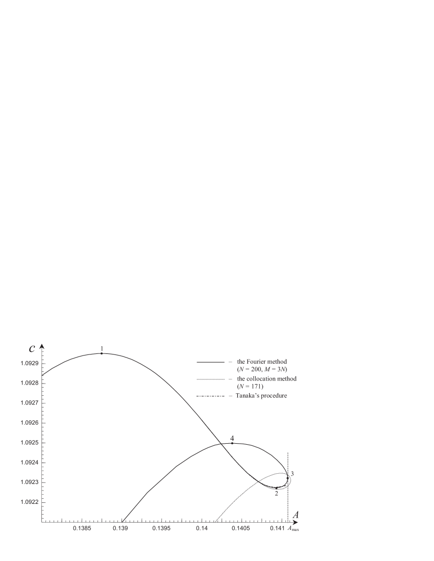
Figure 1: The wave phase speed $c$ of a surface wave versus its steepness $A$.

Table 1: The values of the wave speed $c$ and the mean water level $\eta_{0}$ for the steep Stokes and spike waves with the wave steepness $A$ calculated by the Fourier method. The values without footnotes were calculated at $N=200,~{}M=3N$. The wave speed for the Stokes waves obtained by Tanaka’s procedure Tanaka (1983) are presented to estimate the accuracy of our calculations.

	Stokes wave			spike wave
$A$	$c$	$c_{~{}\text{Tanaka}}$	$\eta_{0}^{(1)}\times 10^{7}$	$c$	$\eta_{0}^{(2)}\times 10^{7}$
0.14	$1.0926149034$	$1.0926149034$	$-2.46\cdot 10^{-10}$	$1.09246$	$-130$
0.1406	$1.09233763$	$1.0923377499$	$-1.31\cdot 10^{-4}$	$1.09249$	$-60$
0.14092	$1.0922742$	$1.0922768392$	$-0.0806$	$1.092422$	$-22.3$
	$1.0922761$		$-0.0221$	$1.092427$	$-17.0$
0.141	$1.0922796$	$1.0922808596$	$-0.385$	$1.092389$	$-15.3$
0.14106	$1.0922949$	$1.0922851047$	$-1.20$	$1.0923548$	$-8.28$
	$1.0922962$		$-1.07$	$1.0923550$	$-7.40$
0.14107	$1.0923008$	$-$	$-1.64$	$1.0923458$	$-6.82$
0.14108	$1.0923114$	$-$	$-2.55$	$1.0923321$	$-4.89$
	$1.0923145$		$-2.45$	$1.0923303$	$-4.08$

The key result of our numerical investigation is that we have revealed a new branch which arises from the point of the limiting steepness in the direction of its decreasing so that the loop 2-3-4 is formed. Thus, the point of the limiting steepness seems to be the point of maximum of $A$, not the breaking point. It should be noted, that firstly we obtained the new branch by the Fourier method, and only after that we could track it by the collocation method using the starting points generated by the first method. As it is shown in Fig. 2, the profile of the new solution near the crest is sharper than the profile of the Stokes wave of the same steepness. Because of this we named it “the spike wave”. The difference between the crests of the Stokes and spike waves becomes stronger as wave steepness drops relative to the limiting value. In Fig. 2 the dashed lines designate the exact local Stokes solution (the Stokes corner flow) which corresponds to the limiting wave with a maximal value of $A$ (point 3 in Fig. 1). In the immediate vicinity of the crest, the profiles of the almost highest Stokes and spike waves asymptotically tend to the dashed lines. This tendency is seen to have the oscillatory character for both waves. For the Stokes waves such oscillations were analytically obtained earlier in Longuet-Higgins and Fox (1977).

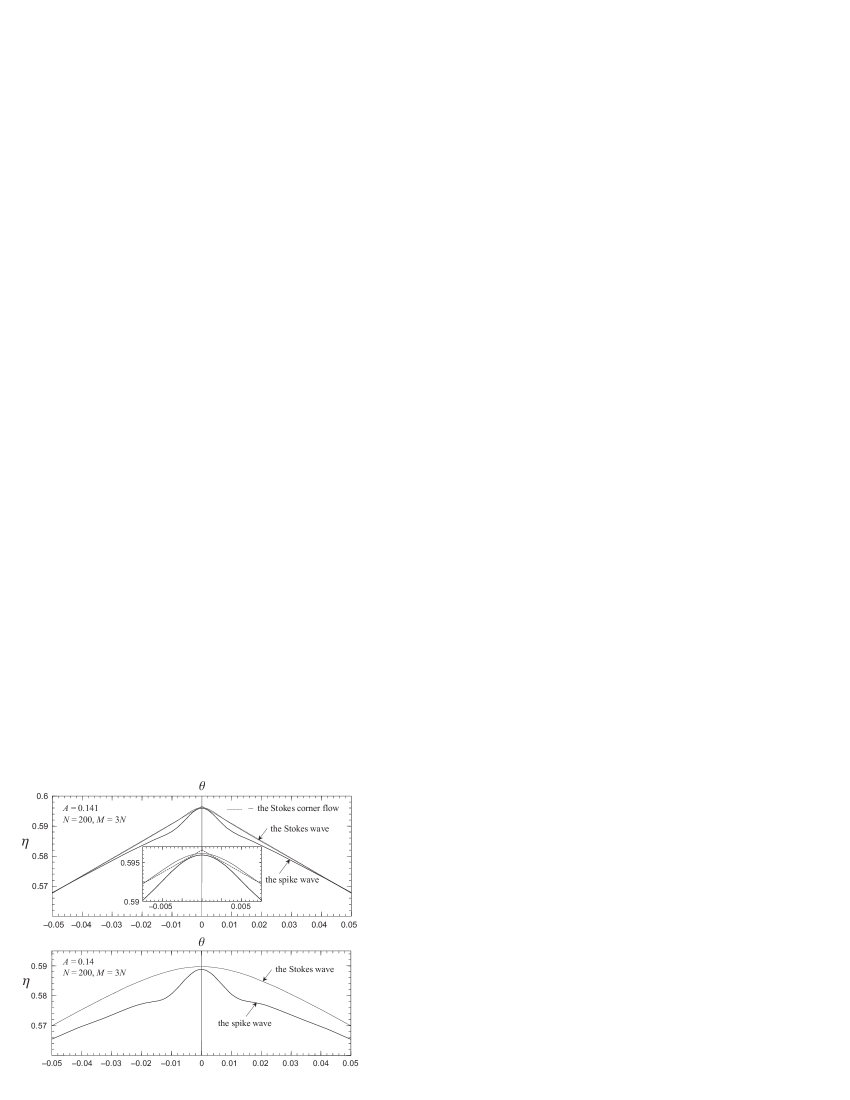
Figure 2: The profiles of a free surface for the Stokes and spike waves of the same steepness and wavelength near the crest.

The values of the wave speed $c$ for the Stokes and spike waves calculated by the Fourier method at different values of wave steepness are presented in Table 1. The high accuracy values of the wave speed for the Stokes branch obtained by using Tanaka’s procedure are also included for comparison. One can see, that for the Stokes branch the accuracy of the Fourier method gradually decreases as wave steepness increases up to the almost highest steepness $A=0.14108$. The correspondent value of the wave speed has only 5 digits stabilized. Note, that Tanaka’s procedure diverges at $A\gtrsim 0.141062$. While moving along the new branch the accuracy becomes still less, and much greater $N$ are needed to stabilize a greater number of digits. As a result, the form of the loop in Fig. 1 has not yet stabilized at $N=200$ and will enlarge with increasing $N$, the cross-section point with the Stokes branch being moved to the left.

Table 1 also demonstrates that besides the form near the crest, the Stokes and spike waves of the same steepness have different mean water levels $\eta_{0}$ relative to the still water level [see Eq. (6)]. One can see, that at the Stokes branch $\eta_{0}^{(1)}$ rapidly descends as $A$ decreases, whereas $\eta_{0}^{(2)}$ increases for spike waves. Analysis of dependences of $\eta_{0}^{(1)}$, $\eta_{0}^{(2)}$ on $N$ and $M$ indicates that they tend to different values at $N,~{}M\rightarrow\infty$.

At the beginning of the paper we assumed the existence of a new type of gravity waves for which the speed of a particle at the crest is greater than wave speed. This property is confirmed by the calculations presented in Table 2.

Table 2: The values of the particle speed at the crest of the Stokes and spike waves of the same wave steepness $A$, in a reference frame moving with wave speed. All values were calculated by the Fourier method at $N=200,~{}M=4N$.

	$q(0)-c$
$A$	Stokes wave	spike wave
0.14092	$-0.0370$	$0.0540$
0.14106	$-0.0121$	$0.0240$
0.14107	$-0.0076$	$0.0194$
0.14108	$-0.0003$	$0.0121$

Thus, the spike waves, which we found numerically using two independent methods, present a new type of gravity waves we looked for. In the present work, we interested only in the existence of new stationary solutions and did not investigate their stability. Profiles of the almost highest Stokes and spike waves differ only in the vicinity of the crest. This leads us to an assumption that excitation of spike waves may possibly be connected with the crest instabilities Longuet-Higgins et al. (1994) of the Stokes almost highest waves. From the other side, sharpening of the crest of a spike wave, when wave steepness decreases (see Fig. 2), makes us look for a relation to a problem of existence of solitary waves on deep water. At present, all existent experimental observations of surface solitary waves on deep water are usually interpreted by excitation of internal waves in stratified ocean Osborne and Burch (1980). However, verification of our assumption demands another numerical algorithm since the ones presented above become ineffective. Finally, two-valued character of a solution of Eq. (1)-(4) in the vicinity of the limiting steepness does not depend on depth, as follows from Eq. (5). We have recently revealed a second branch for a layer of finite depth.